General Circulation Model Downscaling Using Interpolation—Machine Learning Model Combination—Case Study: Thailand

Abstract

Climate change, a global problem, is now impacting human life and nature in many sectors. To reduce the severity of the impacts, General Circulation Models (GCMs) are used for predicting future climate. The prediction output of a GCM requires a downscaling process to increase its spatial resolution before projecting on local area. In order to downscale the output to a higher spatial resolution (less than 20 km), a statistical method is typically considered. By using this method, a large amount of historical observed data, up to 30 years, is essential. In some areas, the historical data is insufficient. Hence, the statistical method may not be suitable to downscale the output on the area which lacks the required data. Hence, this research aims to explore a high spatial resolution downscaling process that is able to provide a valid and high accuracy result in the Thailand area with a limitation in quantity of historical data. In this research, a combination of an interpolation and machine learning model called `IDW-ANN’ is proposed for downscaling the data under the condition. The prediction of temperature and precipitation from a GCM, IPSL-CM6A-LR in CMIP6 is downscaled by the proposed combination into a 1 km spatial resolution. After the performance evaluation, the IDW-ANN downscaling process showed good accuracy (RMSE, MAE, and R²) and valid downscaled results. The future climate situation in Thailand, in particular temperature, and precipitation level, in 2040 and 2100 under two scenarios of SSPs (SSP1-2.6 and SSP3-7.0) is also projected at 1 km resolution by using IDW-ANN. From the projection, the level of precipitation sums, and temperature seem to be increased in most of Thailand in all future scenarios.

1. Introduction

Climate change is a change in climate pattern over the long term [1]. It is the consequence of greenhouse gas emission since the pre-industrial revolution [2]. Climate change is now a problem on a global level which can impact on a local scale. With the change in the level of climate value and its pattern, extreme events, e.g., flash flood or drought, have a probability of occurring with higher frequency [2]. Various sectors, e.g., agriculture, ecosystem, human and food security, and natural resource management, could be threatened by these impacts, which will also lead to huge losses [3,4] It could be said that the impacts of the change in climate could damage the sustainable development of the country. In order to move toward sustainability under these impacts, prompt and precise climate action should be performed urgently in line with SDGs and the thirteenth goal (SDG13) [5,6].

To take action, adaptation is one of the strategies that is used for responding. It mainly focuses on adapting life and preparation to reduce the severity of the impacts from future changes [7]. With the goal of decreasing the extremity on the local level, an assessment of risk and impacts, as well as an adaptation plan for various sectors is typically performed by comparing possible future climate with the current situation [8,9,10,11]. To obtain the future climate situation, a prediction under diverse scenarios from a model called the General Circulation Model (GCM) is used. However, the prediction output of the GCM is at a low spatial resolution (250–600 km). In addition, it contains discrepancies from the prediction at the global level. In other words, the output may not well reflect information on a small local area. This could challenge adaptation activities [12]. Hence, in order to utilize the prediction output, a process for increasing its spatial resolution and calibrating the prediction output named `Downscaling’ is necessary.

In the case that high spatial resolution downscaling (less than 20 km) is desired, the statistical method is most suitable. However, the method may not be functional in some areas in accordance with a prerequisite in historical observed data quantity on the interested area [13,14]. Thailand, a developing country, is also facing insufficient historical data. By considering the prerequisite of statistical downscaling, it is possible to deduce that the situation of the data is a challenge in the high spatial resolution downscaling of the GCM output in the Thailand area. To overcome the challenge, this research aimed to find a method for the downscaling process that is able to provide a valid and accurate result under the limitation of data.

In this research, Inverse Distance Weight (IDW) and an Artificial Neural Network (ANN) were used as methods for increasing spatial resolution and calibrating data, respectively. Both methods have been widely used in various studies for downscaling and provide a satisfactory performance [15,16,17,18,19,20,21,22,23]. Hence, to overcome the limitation in the amount of data for Thailand, this research proposes a framework of the downscaling process that is a combination of the two methods called `IDW-ANN’. To evaluate performance, the prediction of temperature and precipitation from IPSL-CM6A-LR, a GCM, which was at 250 km spatial resolution between 2008–2014 were downscaled to 1 km on Thailand by the proposed framework. Then, the downscaled result is assessed by RMSE and MAE for its accuracy. For validity, a comparison between the result and 30 years of statistical data of normal value was performed. In addition, the IDW-ANN framework was also used to downscale the future prediction of climate under two SSPs scenarios from the Coupled Model Intercomparison Project (CMIP) Phase 6, i.e., SSP1-2.6 and SSP3-7.0 in 2040 and 2100. The downscaled result of the prediction was projected and compared with the historical data to explore the change which may occur in the future.

In this article, four other sections are structured as follows. Section 2, Background, literature on GCM and downscaling, and also the climate change situation in Thailand are described. In Section 3, Materials and Methods, a framework for the IDW-ANN downscaling process is presented. In Section 4, Results, an experiment setting, a performance evaluation, and downscaling results with climate projection are included. In Section 5, Discussion, temperature level and annual precipitation sum projection of Thailand in 2040 and 2100 by using GCMs output under two SSPs scenarios are shown, aimed to explore the change that may occurred in future climate. Finally, Section 6, Conclusions, concludes this research work.

2. Background

2.1. General Circulation Model

The General Circulation Model or Global Climate Model (GCM) is a three-dimensional mathematical model that represents physical processes in the climate system at the global level [13]. By using the model, climate variables, e.g., temperature and precipitation, are predicted over a three-dimensional grid with a resolution of 250–600 km of horizontal and 10–20 vertical layers [24]. In the climate change sector, the GCM is a modern and well-developed tool for stimulating climate system response to the change in greenhouse gas level [25].

For adapting to climate change and sustainable development in the long term, the future climate prediction output from GCMs under scenarios of various conditions, e.g., greenhouse gas emission, land use, and socio-economic situation, plays an important role. With the climate prediction output, it is possible to analyze the impact and its severity that may occur in each sector from the change in climate pattern and capable to plan for prompt response and appropriate management. In this study, a future scenario called ‘Shared Socio-economic Pathways’, which is now used as an input scenario for the GCM, is the focus.

Shared Socio-economic Pathways or SSPs is a simulated scenario that mimics how the different development of socio-economic factors affect or challenge climate change response strategies [26]. SSPs consist of five socio-economic scenarios, SSP1–5, respectively. In this study, GCM output under two socio-economic scenarios, SSP1 and SSP3, were selected. For SSP1, it stimulates that the world slowly shifts towards sustainability, which is a low challenge to climate response. However, in SSP3, regional conflict increases, and countries decide to focus on themselves instead of international cooperation, especially in the environmental sector. Hence, this scenario is a challenge for the climate response at a high level.

However, as mentioned, the output of the GCM named IPSL-CM6A-LR under SSP1-2.6 and SPP3-7.0 was selected in this study. The following number behind the scenarios refers to a radiative forcing in W/m², which may occur in 2100. The radiative forcing is a difference between an incoming and reflecting energy and could be changed by components in the atmosphere, e.g., greenhouse gas [27]. This could be said that SSP1-2.6 is an ideal scenario for climate change situation, while SSP3-7.0 is a worst-case scenario.

Nevertheless, as a consequence of coarse spatial resolution, GCM output could poorly represent data at the local level and render it unsuitable for utilization. To increase the spatial resolution, the downscaling process is essential.

2.2. Downscaling

Typically, the output of GCMs is in a coarse spatial resolution that poorly represents data in a small area. To be specific, it is not suitable for a task that requires a high spatial resolution of climate data for the projection. Hence, the output of GCMs should be increased in spatial resolution. The method for turning it into a finer scale is called `downscaling’.

Downscaling is a technique that is used for increasing the resolution of data. From [13], it is local scaled data (10–100 km spatial resolution) deduction from larger scaled data. Figure 1, on the left side, shows the original data with a spatial resolution of 250 km. When comparing with the right side, which has higher spatial resolution after being downscaled (1 km), the left one has less ability to represent data at the local level. Increasing the resolution consists of two methods: (1) Interpolation for generating value between known data points to increase resolution, and (2) Capturing the relationship between observed data and prediction output historically, which aim to calibrate the prediction.

2.2.1. Interpolation

Interpolation is a procedure for valuating unknown data by considering the surrounding existing data [28]. In this study, spatial interpolation techniques were the focus. The spatial interpolation assumes that the correlation between data points in close range is stronger than far apart points [29]. To interpolate, spatial information is involved in estimating a value where the data does not exist. In Figure 2, an idea of the spatial interpolation is shown. The black points refer to sample points in which the value is collected, while a grey cross-sign is representative of a point in an unsampled area. To estimate the value of an unknown value point, the spatial information, in this case, distance is involved. By the assumption of the spatial interpolation, the estimated value of the unknown value point should be closer to the near sample points than the further points.

Spatial interpolation has been applied for tasks in several branches, e.g., environmental science and ecology. For example, continuous spatial data, which play an important role in various tasks in environmental and ecological sectors, are not usually available in the real world because of the difficulty and expense of the collection process. In other words, there are some areas that may not be included in an exploration. However, continuous spatial data are essential for decision-making, risk assessment, etc. [30]. Hence, spatial interpolation plays an important role in generating data in the unsampled area by using mathematical methods, whether non-geostatistical or geostatistical.

For the interpolation part of this study, a non-geostatistic spatial interpolation named ‘Inverse Distance Weight’ was considered. IDW is a popular method for interpolation due to its ease of use and the small number of parameters to be set (low complexity) [15]. From the literature, performance in climate data estimation of various spatial interpolation methods, including IDW, has been compared in many studies. It shows that the error of the interpolated values by IDW is low-level and not largely distinct from the other methods [15,16,17].

Therefore, because of its ease and low complexity with good performance, IDW was selected to interpolate climate variables data, specifically temperature and precipitation, into a desired scale (1 km) in a downscaling process.

2.2.2. Capturing the Relationship of Data

Capturing the relationship consists of two traditional approaches, dynamic and statistical. In the case of high spatial resolution (<20 km) of data is desired and a statistical approach is more suitable [13]. However, because of its requirement for high quality and quantity of historical observed data (>30 years) of the research area, the statistical approach may not be workable in some localities. In fact, the large amount of historical data of high quality is difficult to obtain in developing countries, which may be caused by station installation, topography, funding, etc. This leads to a challenge in downscaling data on the area that lacks historical data. Moreover, the relationship between observed and predicted output, in some cases, is uncertain through time. Therefore, the method used in the statistical approach may become inapplicable in this situation.

To overcome the limitation of the traditional approach in downscaling data into a high spatial resolution, a machine learning model was selected from the literature. By comparing with a statistical approach, Linear Regression (LR) and Generalized Linear Model (GLM), machine learning models, Artificial Neural Networks (ANN), Support Vector Regression (SVR), Hybrid Support Vector Regression (HSVR), Least-Square Support Vector Machine (LS-SVM), and Gradient Boosting Regression Tree (GBRT) showed better efficiency in downscaling data [18,19,20,21,31].

In the literature, ANN has been widely applied in plenty of climate research, as well as downscaling GCM output for various climate variables. In downscaling, the model shows a satisfactory performance in high accuracy, even with a simple structure, e.g., single hidden layer and feed-forward model [18,19,20,21,22,23]. Thus, to downscale GCM output, ANN was chosen as a machine learning tool that was in charge of capturing the relationship between data in this study.

2.3. Climate Change and Thailand

Thailand, located 15 degrees above the equator, is placed in the center of South East Asia. From the climate standard normal value of Thailand in 30 years, the annual mean temperature level and precipitation sum are 27 °C and 1587.5 mm, respectively.

With the climate change situation, climate patterns on a local scale as in Thailand have been affected. From the late 20th to the early 21st century, the annual average temperature was found to increase around 1 °C. For precipitation, it was found that the annual sum of the amount was varied and led to both drought and flood situations. For example, in 2010, the water level in the Mekong River became the lowest in 50 years because of an extreme drought. The possible cause was determined to be the rainy season in 2009 occurring late but ending early [32]. In addition, according to the Long-Term Climate Risk Index for 2021 by Germanwatch, Thailand was ranked 9th out of 178 for the countries most affected by the change of climate with 146 times increase in natural disasters within 21 years [33].

The change in pattern or level of climate has an opportunity to provide a critical effect on various sectors. The ecosystem in the local area also requires high attention. In fact, the terrestrial biome and climate zone of each area is mainly classified by average annual temperature and precipitation level [34]. The change in these factors could affect the position of the biome and climate zone, which may lead to ecological functionality change in the area. In addition, Thailand is currently a developing country, especially in the agricultural and industrial sectors. The change in climate pattern and its impact on the ecosystem has an opportunity to result in difficulty in production, thus causing a chain effect on economic, human, and food security, as well as impacting the sustainability of the country.

Hence, the preparation for reducing the severity of the impact, to be specific, an adaptation plan, should be considered. To create the plan, future climate simulation under various scenarios from GCM plays a leading role. Nonetheless, the historical observed data, which are essentially for downscaling GCM output to fine spatial resolution, are insufficient in Thailand (data are only available from 2008–the present). To overcome the limitation in data quantity, this study proposed a downscaling process which is a combination of interpolation method and machine learning model called ‘IDW-ANN’.

3. Materials and Methods

3.1. Study Area

Thailand, located at latitude of 15°87′ N and longitude of 100°99′ E, is one of the countries in Southeast Asia. With a total area of 513,120 km², it contains various terrains, including forested mountains, dry plateaus, river plains, and also beaches. From the Automatic Weather System (AWS) of the Thai Meteorological Department (TMD), there are 106 meteorological stations in Thailand, as shown in Figure 3.

3.2. Data

In this study, the data are categorized into 2 parts: observed data and GCMs output. The details of each part are as follows.

3.2.1. Observed Data

For observed data, average temperature and precipitation sum, both monthly, from 106 meteorological stations in Thailand during 2008–2014 (7 years). The data are retrieved from Automatic Weather System, TMD official website (http://www.aws-observation.tmd.go.th/ (accessed on 7 October 2022)). According to the 30-year statistical normal value, the minimum and maximum value of both variables are shown in

Table 1. Minimum and maximum value of an average temperature and precipitation sum, both monthly, from 30-year normal climate value of Thailand.

Variable	Minimum	Maximum
Average temperature (°C)	18.1	34.2
Precipitation sum (mm.)	1.5	1040.4

.

3.2.2. GCM Output

In this study, with the aim of downscaling prediction of temperature and precipitation from the GCM, predicted outputs from IPSL-CM6A-LR in CMIP6 were selected as demonstration data for downscaling [35]. IPSL-CM6A-LR is a GCM developed by Institut Pierre Simon Laplace, France [36]. The GCM provides a prediction in 250 × 250 km² spatial resolution. The selection was decided by the availability of the data. The output in historical (2008–2014) and future (2040 and 2100), under SSP1-2.6 and SSP3-7.0, of 3 variables, i.e., Near-surface air temperature, Precipitation, and Near-surface relative humidity, all monthly, are included. All the outputs of the GCM were provided by Copernicus Climate Change Service, European Commission, and European Centre for Medium-Range Weather Forecasts.

Table 2. Summary of related variables.

Data	Variable	Unit
Observed data	Average temperature	°C
	Precipitation sum	mm
GCM output	Near-surface air temperature	°K
	Precipitation	kg m−2 s−1
	Near-surface relative humidity	percentage

presents a list of variables from both the observed and the GCM output of this research.

3.3. IDW-ANN Downscaling Framework

With the aim to overcome the data downscaling limitations, a downscaling framework by using the combination of the interpolation and machine learning model called ‘IDW-ANN’ is proposed in this study. As presented in Figure 4, three processes, data preprocessing, downscaling, and climate projection, are included in the framework. Details of each process are described as follows.

3.3.1. Data Preprocessing

In this study, the relevant data were all secondary data provided by the Thai Meteorological Department (TMD) and Copernicus. Therefore, the quality of the data was unknown and its format may not have been appropriate for utilization. To assess and handle the quality and characteristics of data, data preprocessing, a process for cleaning data and making it available in the desired format, was essential [37,38].

For the observed data, abnormal values were found in both temperature and precipitation. The abnormality of the value may affect the accuracy of the downscaling process, i.e., the interpolation method may generate an abnormal value which could lead the machine learning model to capture the wrong relationship of data. To handle this, the value which is out of range from the 30-year normal value as shown in Table 1, was excluded from the data.

After an exploration, because the data were provided by different sources, the unit of both climate variables, temperature and precipitation, of the GCM output was different from the observed data, as shown in

Table 3. Comparison of each climate variable unit between two datasets: observed data and GCM output.

Variable	Observed Data	GCM Output
Temperature	°C	°K
Precipitation	mm/month	kg m−2 s−1

. Hence, the unit of data from the GCM output was converted to the same as the observed data.

The last method which was performed in the data preprocessing process was normalization. Normalization is a method to make data values of all variables within the same scale. In this study, Min-Max normalization, which formula is shown in Equation (1), was used to turn data value into a 0–1 scale.

$$X^{\prime }=\frac{X-X_{min}}{X_{max}-X_{min}}$$

(1)

where X is an original value, $X^{\prime }$ is a normalized value, $X_{min}$ is the minimum value of data, and $X_{max}$ is the maximum value of data. Before the preprocessed data were used in the downscaling process, the data were split into two parts: training (data in 2008–2013) and test set (2014).

3.3.2. Downscaling Process

To downscale GCMs output, both observed and prediction from models were interpolated. Then the interpolated data were fed into a machine learning model to capture their relationship. In this study, Inverse Distance Weight (IDW) and an Artificial Neural Network were selected as interpolation and capturing relationship methods for downscaling, respectively.

Interpolation: Inverse Distance Weight (IDW)

After the data were preprocessed, new data points were generated between the existing data by using IDW to increase the spatial resolution to 1 km. To estimate the value of the new point, each existing point was given a weight, considering by spatial distance to the new one. The nearest point, in other words, the point which had the least spatial distance from the new point would receive a larger weight than the others. The estimation was performed by an equation of IDW as shown in Equation (2).

$$z_p=\frac{{\sum }_{i=1}^n\frac{z_i}{d_i^{\beta }}}{{\sum }_{i=1}^n\frac{1}{d_i^{\beta }}},$$

(2)

where $z_p$ refers to the new data at point p, $z_i$ is the value of known data at point i, and $d_i$ means distance between point p and i, and $\beta \in \mathbb{R}$.

As previously mentioned, IDW is a spatial interpolation method. Therefore, distance is one of the factors which affect the interpolated values. Another one is an exponent value, $\beta$. In order to use IDW, $\beta$ is required to be set by the user. To be more specific, $\beta$ is used to determine how surrounding known data points affect the generated value of the unknown. With an increase of $\beta$ value, the nearby data points will become the most influenced and the generated value will be closer to the value of the nearest point (high bias to the near one). In contrast, with the lower value of $\beta$, the further surrounding points will be given more emphasis, leading to the interpolated data becoming smoother than the higher $\beta$ [39,40].

To select the value of $\beta$, the distance and distribution of meteorological stations were considered. Because the distance between stations is quite high and there is no station installation in some areas of Thailand, $\beta$ was set as 1 to in this study to increase the influence of further surroundings data points on the generated values.

Capturing relationship: Artificial Neural Network

The interpolation of the prediction output cannot be used directly due to its discrepancy. In order to calibrate the value, capturing the relationship between the interpolated data, both observed and the output is essential. In this research, Artificial Neural Network or ANN is selected as a capturing method. ANN is a computational weighted graph, inspired by biological neural networks [41]. To simplify, it is a nonlinear model which simulates the human brain process. It has the ability to solve complicated relationships by using nonlinear model calibration [42,43]. Typically, ANNs consist of three types of layers: input, hidden, and output, with connected nodes [44]. Each node, in any layer, works as an input receiver, result aggregator, and output sender for the next layer. To send out the output, it is based on an activation function of each layer. The activation function is an imitator of synapses in the human brain. The node will only send the result to the next layer only if the signal is strong enough to activate the function.

In order to capture the relationship between observed data and GCM output, two ANN models were built and trained separately, one for temperature and one for precipitation. To select the variable as the input of each model, the correlation between the variables in the historical observed data was considered. Figure 5 shows the correlation between variables from the historical observed data, computed by Pearson’s correlation. For the average temperature, altitude was the only variable that has a correlation at a moderate level (−0.5). However, in accordance with the availability of the data, an elevation from DEM was used instead of the altitude. For precipitation, it rarely showed a correlation with the other variables. The highest value of correlation turned out to be humidity with a weak level (0.3). After considering the correlation, the set of variables, both historical and GCM output as shown in the

Table 4. List of model inputs for downscaling each climate variable.

Climate Variable	Observed Variable	GCMs Output Variable	Others
Temperature	Average temperature	Near-Surface air temperature	Digital Elevation Model (DEM) Month
Precipitation	Precipitation sum	1. Precipitation 2. Near-Surface relative humidity	Month

were included for model training. For further information, the month was also added as the input to be a seasonal variable.

With the set of inputs, each model contains a slightly different structure, as shown in Figure 6 and Figure 7. In this study, only a single hidden layer was added to the models, because the number of the inputs is not large. To train the models and evaluate their performance, the interpolated data, all variables of both the observed and output, were divided into three sets, i.e., train (2008–2012), validation (2013), and test set (2014). The training of the model was done by using Tensorflow (https://www.tensorflow.org/ (accessed on 20 November 2022)) and Keras tuner (https://keras.io/keras_tuner/ (accessed on 29 November 2022)).

Downscaling process setup

In order to use IDW and ANN for downscaling process, a few parameters were required to be set. The list of parameters and their values are presented in

Table 5. List of parameters and their values in IDW and ANN.

Method	Parameter	Temperature	Precipitation
IDW	$\beta$	1	1
ANN	The number of hidden layers	1	1
	The number of nodes in hidden layer	4	5
	Learning rate	0.2	0.002
	Optimizer	SGD	RMSprop
	Epoch	110	60
	Batch size	145,000	104,000
	Seed	42	42

. Note that the parameters of each ANN model were set separately.

3.3.3. Climate Projection

After the downscaling process was done, the downscaled results in historical were projected over the Thailand area, aiming to evaluate its validity. In addition, the predicted climate in the future, 2040 and 2100, under two scenarios from GCM were able to be projected to explore the change that might occur. However, the results from the downscaling process were not in an appropriate format for projecting.

To project the downscaled results, a few methods were involved. Firstly, as described in data preprocessing, both observed data and GCM output were normalized. This could be because the results from the downscaling were also normalized values. Therefore, the values were required to be denormalized before the projection to present the real value. Then, the set of denormalized values was merged with geometry information of its location to create shapefiles. Lastly, climate maps were projected over Thailand using the shapefiles on QGIS version 3.24.

3.4. Performance Metrices

3.4.1. Accuracy Evaluation

To evaluate the performance of IDW-ANN downscaling process, RMSE, MAE, and R² were used as metrics to measure the accuracy of predicted results by comparing them with the real data from meteorological data of Thailand. The detail and equation of each metric are available as follows.

• Root Mean Squared Error or RMSE is typically used for estimating a standard deviation of residual distribution. RMSE could be computed by Equation (3).

  $$RMSE=\sqrt{{\displaystyle \sum _{i=1}^n}\frac{{({\widehat{y}}_i-y_i)}^2}{n}}$$

  (3)

  where $y_i$ is the observations value, ${\widehat{y}}_i$ is the predicted value and n is number of observations.
• Mean Absolute Error or MAE is a linear score that is used for measuring an average of an absolute error [45]. With MAE, all the errors are weighted equally, and its score is increased by the increase in the error. The MAE score could be calculated by Equation (4).

  $$MAE=\sum _{i=1}^n\frac{|y_i-{\widehat{y}}_i{|}^2}{n}$$

  (4)

  where $y_i$ is the observations value, ${\widehat{y}}_i$ is the predicted value, and n is the number of observations.
• Coefficient of determination or R² is typically used to reflect how large the proportion of variance of the target that the model could explain [46]. The R² could be calculated by Equation (5).

  $$R^2=1-\frac{{\sum }_{i=1}{(y_i-{\widehat{y}}_i)}^2}{{\sum }_{i=1}{(y_i-\overline{y})}^2}$$

  (5)

  where $y_i$ is the value of the observation, ${\widehat{y}}_i$ is the predicted value and $\overline{y}$ is the average of the observation values.

3.4.2. Result Validity

For the purpose of producing downscaled data that is highly close to the actuality of climate in Thailand, the results from the downscaling process were required to be examined. For checking validity, the results, both temperature and precipitation, were compared to statistical data for 30-year (1991–2020) normal value of Thailand, provided by TMD.

4. Results

4.1. Performance Evaluation

4.1.1. Downscaled Data Validity

To evaluate the validity of the downscaled results, the mean of an average temperature and precipitation sum, both annual, were compared with the 30-year normal value of the climate in Thailand, which was obtained from the meteorological stations. The comparison results of both climate variables are shown in

Table 6. Comparison between normal value of climate variables (30 years) of Thailand and downscaled result from IDW.

Variable	Normal Value	IDW-ANN	Difference
Average temperature	27	26.8	−0.2
Precipitation sum	1587.5	1718.48	130.98

.

4.1.2. IDW-ANN Accuracy

At the stage of capturing the data relationship, the ANN was trained by using the IDW interpolated data from 2008–2012 and validated by the data in 2013. To evaluate its accuracy, the prediction on the training data (2008–2012), validation (2013) and test data (2014) were measured with the historical observed data from 106 stations in Thailand by using three metrics: RMSE, MAE, and R². The evaluation result is shown in

Table 7. IDW-ANN performance evaluation on training (2008–2012), validation (2013), and test set (2014).

Metrics	Temperature			Precipitation
	Train	Validation	Test	Train	Validation	Test
R2	0.7571	0.7458	0.7322	0.7045	0.7216	0.7013
RMSE	0.0909	0.0975	0.0891	0.0457	0.0463	0.0369
MAE	0.0617	0.0673	0.0616	0.0306	0.0311	0.0271

. For more information, test data were a blind dataset that the model had never seen. In other words, the test set was not included in the training process.

The evaluation shows that all RMSE and MAE scores are in the same way. The scores of the models are lower than 0.1 for all data sets, as shown in Table 7. For the temperature model, RMSE scores are 0.0909, 0.0975, and 0.0891 and MAE scores are 0.0617, 0.0673, and 0.0616. For R², the scores are 0.7571, 0.7458, and 0.7322. The scores for precipitation are 0.0457, 0.0463, and 0.0369 for RMSE and 0.0306, 0.0311, and 0.0271 for MAE. Lastly, R², the scores are 0.7045, 0.7216, and 0.7013.

4.2. Climate Projection on Thailand Area

By using IDW-ANN, the GCM output downscaling results at 1 km spatial resolution were projected over Thailand area for both historical (2008–2014) and future (2040 and 2100). In the case of the future period, the future climate under two scenarios, i.e., SPP1-2.6 and SSP3-7.0, were projected to display the change which may occur. All the downscaling results, the value of difference, and the absolute difference are shown in Figure 8, Figure 9, Figure 10, Figure 11, Figure 12 and Figure 13.

5. Discussion

5.1. Performance of the IDW-ANN Framework

To evaluate the performance of the proposed framework, two metrics were involved. For validity, the annual downscaled result was compared with the 30-year normal value, as shown in Table 6. The slight difference appeared in the average temperature. IDW-ANN provided a result lower than the normal value of 0.2 °C. In contrast, the given result in precipitation sum was higher than the statistic of 130.98 mm.

For accuracy, the scores of all metrics for the IDW-ANN did not exceed 0.1 in all data sets and variables. Please note that for RMSE and MAE, the lower score means the better. According to Table 7, the scores of validation were higher than the others, but still in the same range as the training and test set. For R², as described previously, it is a reflection of how much the model could explain the variance of the target value, in this case, climate value. In addition, the greater score of R² was better. From the evaluation, the R² scores of IDW-ANN downscaled results, both temperature and precipitation, were around 0.7–0.75. Therefore, it could be concluded that IDW-ANN quite does well in calibrating the prediction from the GCM, both for temperature and precipitation.

Considering the evaluation, it could be said that IDW-ANN is able to downscale GCM output in the historical period to be close to the actual values from the observed data, even though the downscaled result showed a higher value than the normal value of the mean annual precipitation sum. In addition, RMSE, MAE, and R² of all data sets are not distinctly different. Therefore, the models seem not to be overfitted to the training set. With all the results, it could be concluded that IDW-ANN has the ability to downscale the output of the GCM with low error under the limitation of data quantity.

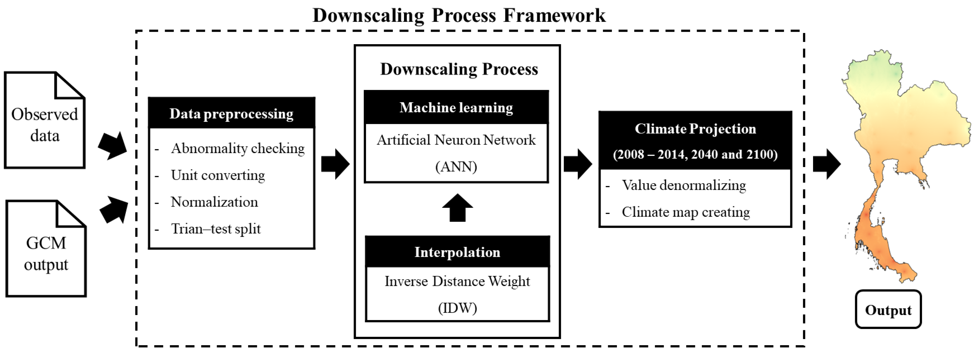
In Thailand, there have been a few previous studies about downscaling GCM output, mostly for precipitation [47,48]. These studies were performed on different scales, number of stations, and data sets. Nevertheless, when compared with the studies methods, the proposed IDW-ANN is less complex by using a smaller number of input variables for calibrating the GCM output. In addition, the downscaling process in this research did not involve a reanalysis of data.

By using the IDW-ANN, the framework is quite flexible for downscaling the output into high spatial resolution. It is able to be applied for downscaling data for another desired resolution under the limitation of historical observed data. However, in order to apply the framework to downscale another climate model or to downscale another area, the parameter setting of the methods may require a new set.

Moreover, as presented in all the figures of climate projection, dark and light spots appear. This is caused by the interpolation method. As described, IDW is the spatial interpolation that uses the distance between points for estimating the newly generated value. Hence, the newly generated points which close to the existing ones usually have a higher similarity than the furthers as shown in the presented figures. Even if it does not affect the accuracy and validity of the results, it should be smoother.

5.2. Comparison of Climate Situation: History (2008–2014) and Future (2040 and 2100)

According to the GCM output downscaling by using the IDW-ANN downscaling process, there are visible differences between the results in historical (2008–2014), a baseline in this study, and the two future scenarios (SSP1-2.6 and SSP3-7.0) in 2040 and 2100. The details of the change in both climate variables of all scenarios are described as follows.

With the downscaling result in the historical data, the annual precipitation sums from 2008–2014 show the average overall area at 1718.48 mm. The lowest level of precipitation was 1393.86 mm, while the maximum was 2181.78 mm. According to Figure 8a, the level of precipitation in the lower half part of Thailand was higher than in the upper. The sum of precipitation was mostly higher than 1512.50 mm annually, with only small amounts of the area at the top, which is less than the value. In the same way, the annual average temperature of the same period shows a similar pattern. The average temperature in the upper part of Thailand was less than 26.5 °C, cooler than the remaining parts and the highest level occurs in the south (higher than 27.0 °C ), as shown in Figure 11a. This could be because the precipitation and temperature level of Thailand are both typically high in the southern part, but low in the northern. However, in 2040 and 2100, the pattern of the climate variables shows a distinct difference. By using ANOVA, both the annual precipitation sums and the average temperature of the two future scenarios are significantly different from the historical data with 95 percent of confidence level.

Starting with SSP1-2.6, an ideal scenario with low radiative forcing, an average of overall annual precipitation sums in 2040 has an opportunity to be higher than the historical. In Figure 10a, a huge difference between the scenario and historical mostly occurs in the upper area. For the upper, the precipitation has increased, especially in the northern region. In contrast, in the south, a decrease occurs instead. While in 2100, the average precipitation in the country level is also likely to be increased from the historical but decreased from 2040 in the same scenario. Even though the pattern of the precipitation in 2100 is similar to the historical data, as shown in Figure 8c, the difference map in Figure 9a shows that most of the area may face a situation of the decreasing the precipitation levels in the next 80 years.

For the temperature, in 2040, most areas show a similar level in pattern with the historical data, which is in the range of 26.5 to 28.0 °C. According to Figure 12a, the temperature level in the upper part may be higher than the historical data up to 0.36 °C but seems to be decreased in the half lower part. Moreover, from the absolute value of the difference, the high level of change in temperature mostly occurred in the upper of the country (+/−0.17–+/−0.52). With the same scenario in 2100, the high level of temperature is expanded from the south to the north. To be simplified, most of the area has a chance to be hotter than the historical data. Compared with 2040, the amount of area with less than 26.5 °C seems to be slightly decreased. According to Figure 11c, the temperature in the upper of Thailand may increase from around 0.19 to 0.36 °C, which is higher than the other area. In the same way, the difference value between the historical and 2100 in temperature at the same area is also highest in the scenario as shown in Figure 12b.

With the worst scenario, the SSP3–7.0, the average of the annual precipitation sums is also higher than the historical for both 2040 and 2100, at 28 and 115 mm, respectively. In 2040, some parts in the central show a decrease in the precipitation level. At the same time, the area which may have precipitation of more than 1850.00 mm is more apparent in the south. For 2100, Figure 8e shows a distinct difference in the precipitation level from all scenarios and all periods. The prediction indicates that the precipitation level may become higher in most areas of Thailand, especially in the upper part. Compared with the historical data, a small change mostly appears in the south with less than 105.75 mm of the absolute different value as shown in Figure 10d. While in the central area, there is a chance that the precipitation may increase up to 176.25 mm or more for the northern part.

In accordance with Figure 11d, the temperature level of most areas in 2040 may become higher than 26.5 °C. The top part of Thailand may face a huge change in the range of 0.25–0.70 of the absolute value of the difference, which is shown in Figure 13c. In contrast, the change seems to be smaller in the lower part. However, the pattern of the temperature level in 2100 is obviously distinct from all scenarios and periods. The prediction in Figure 11e shows that the temperature of all areas will be increased from the historical. Even the temperature in the top is cooler than the others, but still higher than the historical around 1 °C. From Figure 12d, it could be said that the high level of temperature is expanded and shifted from the lower to the upper. Moreover, Figure 13d displays that the temperature level of all areas in 2100 under the SSP3-7.0 scenario probably changes at a huge level, especially in the upper part.

By comparing two future scenarios, the changes in both climate variables in 2040 under the scenarios and 2100 under SSP1-2.6 are similar. For the annual precipitation level, the northern area shows a decrease in value. In addition, the pattern of the precipitation level distribution seems to have shifted downward, while the temperature shows an inverse pattern. From the result in Figure 11, the temperature level distribution pattern probably shifts from southern to northern. To be specific, the three situations predict that the temperature in the upper part of Thailand will be higher than the historical data. Nevertheless, the prediction of precipitation and temperature in 2100 under SSP3-7.0 is in a distinctly different pattern. An enormous increase in both variables in all areas of Thailand is predicted to occur. It could be said that the situation in 2100 under SSP3-7.0 is representative of the worst case scenario.

According to the prediction from the GCM under two future scenarios, the northern area of the country should be given high attention, also prompt planning for the adaptation, and response is essential. As presented in the results, the northern part of Thailand has an opportunity to face the change in the level of climate variables more severe than the other area in the same period and scenario. The precipitation in the north is predicted to be increasing in all scenarios, especially in 2040 under SSP1-2.6 and 2100 under SSP3-7.0. In the same way, the temperature level will also probably become higher.

Considering the present world situation, it is quite similar to the stimulated socio-economic scenario of SSP3, e.g., the occurrence of regional conflicts. Therefore, it could be said there is a probability that the situation in SPP3-7.0 will occur in the next 20 years, 2040. With the projections, the annual precipitation level tends to increase, in line with the average temperature. The change in climate level has a probability to impact on ecosystems of the country. In fact, the terrestrial biome is mainly classified by temperature and precipitation [34]. Therefore, the change of these variables may affect the position of biome and may threaten natural resource and food security [49,50,51]. Therefore, in order to be prepared for the change of climate, a climate change response of Thailand based on the worst scenario is suggested to be planned. To reduce the severity of the impact which probably occurred from the change, a comprehensive and practical adaptation plan which covers all important sectors of human beings and natural management is necessary and should be published by the government and related organizations. In addition, an explicit climate action should be included in the development plan of the country. Moreover, greenhouse gas emissions reduction is also important and should be performed along with the preparation for the future.

6. Conclusions

In this study, a combination of interpolation and machine learning called ‘IDW-ANN’ was proposed for downscaling the output of the GCM into high spatial resolution, aiming to overcome a challenge in the lack of historical climate data in Thailand. By using IDW-ANN, the prediction outputs of precipitation sums and average temperature, both annual, in historical (2008–2014), and under two future scenarios, SSP1-2.6 and SSP3-7.0, were downscaled into 1 km spatial resolution. In accordance with the evaluation of the downscaling process, IDW-ANN shows a satisfactory performance in both downscaled data validity and accuracy. Considering the two metrics, validity and accuracy, it could be concluded that the proposed IDW-ANN has the ability to downscale GCM output under the limitation in the amount of observed data. Nevertheless, the framework is limited to the two variables -temperature and precipitation. For future work, downscaling other variables, also applying them to another area are considered.

With downscaled GCM output under future scenarios, there is an opportunity that all areas in Thailand will face changes in precipitation and temperature level. All future scenarios show that the sum of precipitation and temperature on average will be increased in most of the area. By comparing all the scenarios, SSP3-7.0 presents the extreme change in precipitation and temperature in 2100. According to the prediction of future climate, as shown in the results, Thailand should be prepared for responding to the change, to reduce the damage of the incoming impact. Hence, the adaptation plan, as well as comprehensive and prompt climate action, is necessary for reducing the severity of the impact, especially in case the worst scenario, SSP3-7.0, occurs.

References

1. United Nations Framework Convention on Climate Change. UN Climate Change Annual Report 2019; United Nations Framework Convention on Climate Change: Bonn, Germany, 2020. [Google Scholar]
2. Intergovernmental Panel on Climate Change. Climate Change 2014 Synthesis Report; IPCC: Geneva, Switzerland, 2014. [Google Scholar]
3. United States Environmental Protection Agency. Climate Change Impacts by Sector. 2022. Available online: https://www.epa.gov/climateimpacts/climate-change-impacts-sector (accessed on 25 May 2023).
4. United Nations. Climate Action and Synergies. 2023. Available online: https://sdgs.un.org/topics/climate-action-synergies (accessed on 25 May 2023).
5. United Nations Development Programme. Sustainable Development Goals. 2023. Available online: https://www.undp.org/sustainable-development-goals (accessed on 27 March 2023).
6. United Nations. Secretary-General’s Briefing to the General Assembly on Priorities for 2023. 2023. Available online: https://www.un.org/sg/en/content/sg/statement/2023-02-06/secretary-generals-briefing-the-general-assembly-priorities-for-2023-scroll-down-for-bilingual-delivered-all-english-and-all-french-versions (accessed on 25 May 2023).
7. Pörtner, H.O.; Roberts, D.C.; Poloczanska, E.; Mintenbeck, K.; Tignor, M.; Alegría, A.; Craig, M.; Langsdorf, S.; Löschke, S.; Möller, V.; et al. 2022: Summary for Policymakers; IPCC: Geneva, Switzerland, 2022. [Google Scholar]
8. Miao, L.; Li, S.; Zhang, F.; Chen, T.; Shan, Y.; Zhang, Y. Future drought in the dry lands of Asia under the 1.5 and 2.0 C warming scenarios. Earth Future 2020, 8, e2019EF001337. [Google Scholar] [CrossRef]
9. Liu, B.; Gao, X.; Ma, J.; Jiao, Z.; Xiao, J.; Hayat, M.A.; Wang, H. Modeling the present and future distribution of arbovirus vectors Aedes aegypti and Aedes albopictus under climate change scenarios in Mainland China. Sci. Total Environ. 2019, 664, 203–214. [Google Scholar] [CrossRef] [PubMed]
10. Buras, A.; Menzel, A. Projecting tree species composition changes of European forests for 2061–2090 under RCP 4.5 and RCP 8.5 scenarios. Front. Plant Sci. 2019, 9, 1986. [Google Scholar] [CrossRef] [Green Version]
11. Toot, R.; Frelich, L.E.; Butler, E.E.; Reich, P.B. Climate-biome envelope shifts create enormous challenges and novel opportunities for conservation. Forests 2020, 11, 1015. [Google Scholar] [CrossRef]
12. Gebrechorkos, S.H.; Hülsmann, S.; Bernhofer, C. Statistically downscaled climate dataset for East Africa. Sci. Data 2019, 6, 31. [Google Scholar] [CrossRef] [Green Version]
13. Trzaska, S.; Schnarr, E. A Review of Downscaling Methods for Climate Change Projections; United States Agency for International Development: Washington, DC, USA, 2014.
14. Hadi, A.F.; Riski, A.; Anggraeni, D.; Saputra, M.D. Principal Component Regression in Statistical Downscaling with Missing Value for Daily Rainfall Forecasting. Int. J. Quant. Res. Model. 2021, 2, 139–146. [Google Scholar]
15. Tewolde, M.G.; Beza, T.A.; Costa, A.C.; Painho, M. Comparison of different interpolation techniques to map temperature in the southern region of Eritrea. In Proceedings of the 13th AGILE International Conference on Geographic Information Science 2010, Guimarães, Portugal, 11–14 May 2010; pp. 1–5. [Google Scholar]
16. Kim, S.N.; Lee, W.K.; Shin, K.I.; Kafatos, M.; Seo, D.J.; Kwak, H.B. Comparison of spatial interpolation techniques for predicting climate factors in Korea. For. Sci. Technol. 2010, 6, 97–109. [Google Scholar] [CrossRef] [Green Version]
17. Chen, F.W.; Liu, C.W. Estimation of the spatial rainfall distribution using inverse distance weighting (IDW) in the middle of Taiwan. Paddy Water Environ. 2012, 10, 209–222. [Google Scholar] [CrossRef]
18. Rahimikollu, J. Application of Neural Network Techniques to Downscale Precipitation. Master’s Thesis, West Virginia University, Morgantown, WV, USA, 2014. [Google Scholar]
19. Duhan, D.; Pandey, A. Statistical downscaling of temperature using three techniques in the Tons River basin in Central India. Theor. Appl. Climatol. 2015, 121, 605–622. [Google Scholar] [CrossRef]
20. Mouatadid, S.; Easterbrook, S.; Erler, A.R. A machine learning approach to non-uniform spatial downscaling of climate variables. In Proceedings of the 2017 IEEE International Conference on Data Mining Workshops (ICDMW), New Orleans, LA, USA, 18–21 November 2017; pp. 332–341. [Google Scholar]
21. Liu, Y.; Feng, J.; Yang, Z.; Hu, Y.; Li, J. Gridded statistical downscaling based on interpolation of parameters and predictor locations for summer daily precipitation in North China. J. Appl. Meteorol. Climatol. 2019, 58, 2295–2311. [Google Scholar] [CrossRef]
22. Laddimath, R.; Patil, N. Statistical Downscaling of Precipitation Data Using Artificial Neural Network. In Proceedings of the International Conference & Exhibition on Best Practices for Sustainable Water, Wastewater & Energy Management, SWWEM-2016, Bangalore, India, 7–9 January 2016. [Google Scholar]
23. Nourani, V.; Jabbarian Paknezhad, N.; Sharghi, E.; Khosravi, A. Estimation of prediction interval in ANN-based multi-GCMs downscaling of hydro-climatologic parameters. J. Hydrol. 2019, 579, 124226. [Google Scholar] [CrossRef]
24. Jalota, S.; Vashisht, B.; Sharma, S.; Kaur, S. Chapter 2—Climate Change Projections. In Understanding Climate Change Impacts on Crop Productivity and Water Balance; Jalota, S., Vashisht, B., Sharma, S., Kaur, S., Eds.; Academic Press: Cambridge, MA, USA, 2018; pp. 55–86. [Google Scholar] [CrossRef]
25. Intergovernmental Panel on Climate Change. What Is a GCM? Available online: https://www.ipcc-data.org/guidelines/pages/gcm_guide.html (accessed on 25 April 2023).
26. Riahi, K.; Van Vuuren, D.P.; Kriegler, E.; Edmonds, J.; O’neill, B.C.; Fujimori, S.; Bauer, N.; Calvin, K.; Dellink, R.; Fricko, O.; et al. The Shared Socioeconomic Pathways and their energy, land use, and greenhouse gas emissions implications: An overview. Glob. Environ. Chang. 2017, 42, 153–168. [Google Scholar] [CrossRef] [Green Version]
27. Massachusetts Institute of Technology. Radiative Forcing. 2020. Available online: https://climate.mit.edu/explainers/radiative-forcing (accessed on 10 May 2023).
28. Florinsky, I.V. Chapter 3—Digital Elevation Models. In Digital Terrain Analysis in Soil Science and Geology, 2nd ed.; Florinsky, I.V., Ed.; Academic Press: Cambridge, MA, USA, 2016; pp. 77–108. [Google Scholar]
29. Li, L.; Tong, W.; Piltner, R. Spatiotemporal interpolation methods for air pollution. In Spatiotemporal Analysis of Air Pollution and Its Application in Public Health; Elsevier: Amsterdam, The Netherlands, 2020; pp. 153–167. [Google Scholar]
30. Li, J.; Heap, A.D. A Review of Spatial Interpolation Methods for Environmental Scientists; Geoscience Australia: Canberra, Australia, 2008.
31. Asadollah, S.B.H.S.; Sharafati, A.; Shahid, S. Application of ensemble machine learning model in downscaling and projecting climate variables over different climate regions in Iran. Environ. Sci. Pollut. Res. 2022, 29, 17260–17279. [Google Scholar] [CrossRef] [PubMed]
32. Marks, D. Climate change and Thailand: Impact and response. Contemp. Southeast Asia 2011, 33, 229–258. [Google Scholar] [CrossRef]
33. Eckstein, D.; Künzel, V.; Schäfer, L. The Global Climate Risk Index 2021; Germanwatch: Bonn, Germany, 2021. [Google Scholar]
34. Stiling, P. Ecology: Global Insights & Investigations; McGraw-Hill: New York, NY, USA, 2012. [Google Scholar]
35. Eyring, V.; Bony, S.; Meehl, G.A.; Senior, C.A.; Stevens, B.; Stouffer, R.J.; Taylor, K.E. Overview of the Coupled Model Intercomparison Project Phase 6 (CMIP6) experimental design and organization. Geosci. Model Dev. 2016, 9, 1937–1958. [Google Scholar] [CrossRef] [Green Version]
36. Boucher, O.; Denvil, S.; Levavasseur, G.; Cozic, A.; Caubel, A.; Foujols, M.; Meurdesoif, Y.; Cadule, P.; Devilliers, M.; Ghattas, J.; et al. IPSL IPSL-CM6A-LR model Output Prepared for CMIP6 CMIP Historical. Version 20180803. Earth System Grid Federation. Available online: https://www.wdc-climate.de/ui/cmip6?input=CMIP6.CMIP.IPSL.IPSL-CM6A-LR.historical (accessed on 25 April 2023).
37. Gupta, V.; Sachdeva, S.; Dohare, N. Chapter 8—Deep similarity learning for disease prediction. In Trends in Deep Learning Methodologies; Piuri, V., Raj, S., Genovese, A., Srivastava, R., Eds.; Hybrid Computational Intelligence for Pattern Analysis; Academic Press: Cambridge, MA, USA, 2021; pp. 183–206. [Google Scholar] [CrossRef]
38. Al-jabery, K.K.; Obafemi-Ajayi, T.; Olbricht, G.R.; Wunsch, D.C., II. 2—Data preprocessing. In Computational Learning Approaches to Data Analytics in Biomedical Applications; Al-jabery, K.K., Obafemi-Ajayi, T., Olbricht, G.R., Wunsch, D.C., II, Eds.; Academic Press: Cambridge, MA, USA, 2020; pp. 7–27. [Google Scholar] [CrossRef]
39. GISGeography. Inverse Distance Weighting (IDW) Interpolation. 2023. Available online: https://gisgeography.com/inverse-distance-weighting-idw-interpolation/ (accessed on 25 April 2023).
40. Esri. How IDW Works. Available online: https://pro.arcgis.com/en/pro-app/latest/tool-reference/spatial-analyst/how-idw-works.htm (accessed on 25 April 2023).
41. Park, Y.S.; Lek, S. Artificial neural networks: Multilayer perceptron for ecological modeling. Dev. Environ. Model. 2016, 28, 123–140. [Google Scholar]
42. Antunes, E.; Vuppaladadiyam, A.K.; Sarmah, A.K.; Varsha, S.; Pant, K.K.; Tiwari, B.; Pandey, A. Application of biochar for emerging contaminant mitigation. Adv. Chem. Pollution, Environ. Manag. Prot. 2021, 7, 65–91. [Google Scholar]
43. Sadiq, R.; Rodríguez, M.J.; Mian, H.R. Empirical Models to Predict Disinfection By-Products (DBPs) in Drinking Water: An Updated Review. In Encyclopedia of Environmental Health; Elsevier: Oxford, UK, 2019; pp. 324–338. [Google Scholar]
44. Mohseni-Dargah, M.; Falahati, Z.; Dabirmanesh, B.; Nasrollahi, P.; Khajeh, K. Machine learning in surface plasmon resonance for environmental monitoring. In Artificial Intelligence and Data Science in Environmental Sensing; Academic Press: Cambridge, MA, USA, 2022; pp. 269–298. [Google Scholar]
45. Schneider, P.; Xhafa, F. Anomaly Detection and Complex Event Processing Over IoT Data Streams: With Application to EHealth and Patient Data Monitoring; Academic Press: Cambridge, MA, USA, 2022. [Google Scholar]
46. Chicco, D.; Warrens, M.J.; Jurman, G. The coefficient of determination R-squared is more informative than SMAPE, MAE, MAPE, MSE and RMSE in regression analysis evaluation. PeerJ Comput. Sci. 2021, 7, e623. [Google Scholar] [CrossRef]
47. Anuchaivong, P.; Sukawat, D.; Luadsong, A. Statistical downscaling for rainfall forecasts using modified constructed analog method in Thailand. Sci. World J. 2017, 2017, 1075868. [Google Scholar] [CrossRef] [Green Version]
48. Chotamonsak, C.; Salathé, E.; Kreasuwun, J. Dynamical downscaling of Global Climate Model over Thailand using Regional Climate Model. In Proceedings of the ICRC-CORDEX 2016, Stockholm, Sweden, 17–20 May 2016. [Google Scholar]
49. Malhi, Y.; Franklin, J.; Seddon, N.; Solan, M.; Turner, M.G.; Field, C.B.; Knowlton, N. Climate change and ecosystems: Threats, opportunities and solutions. Phil. Trans. R. Soc. B 2020, 375, 20190104. [Google Scholar] [CrossRef] [Green Version]
50. Dobrowski, S.Z.; Littlefield, C.E.; Lyons, D.S.; Hollenberg, C.; Carroll, C.; Parks, S.A.; Abatzoglou, J.T.; Hegewisch, K.; Gage, J. Protected-area targets could be undermined by climate change-driven shifts in ecoregions and biomes. Commun. Earth Environ. 2021, 2, 198. [Google Scholar] [CrossRef]
51. Grimm, N.B.; Chapin, F.S., III; Bierwagen, B.; Gonzalez, P.; Groffman, P.M.; Luo, Y.; Melton, F.; Nadelhoffer, K.; Pairis, A.; Raymond, P.A.; et al. The impacts of climate change on ecosystem structure and function. Front. Ecol. Environ. 2013, 11, 474–482. [Google Scholar] [CrossRef] [Green Version]
Figure 1. Comparison between non-downscaled (left) and downscaled data (right).
Sustainability 15 09668 g001
Figure 2. An example of spatial interpolation.
Sustainability 15 09668 g002
Figure 3. Study area and station distribution.
Sustainability 15 09668 g003
Figure 4. Framework of IDW-ANN downscaling method.
Sustainability 15 09668 g004
Figure 5. Correlation between climate variables.
Sustainability 15 09668 g005
Figure 6. ANN structure for downscaling temperature.
Sustainability 15 09668 g006
Figure 7. ANN structure for downscaling precipitation.
Sustainability 15 09668 g007
Figure 8. Annual precipitation sum of (a) 2008–2014 (b) 2040 under SSP1-2.6 (c) 2100 under SSP1-2.6 (d) 2040 under SSP3-7.0 and (e) 2100 under SSP3-7.0.
Sustainability 15 09668 g008
Figure 9. Difference in the annual precipitation sum between the historical data and (a) 2040 under SSP1-2.6 (b) 2100 under SSP1-2.6 (c) 2040 under SSP3-7.0 and (d) 2100 under SSP3-7.0.
Sustainability 15 09668 g009
Figure 10. Absolute difference in the annual precipitation sum between the historical data and (a) 2040 under SSP1-2.6 (b) 2100 under SSP1-2.6 (c) 2040 under SSP3-7.0 and (d) 2100 under SSP3-7.0.
Sustainability 15 09668 g010
Figure 11. Annual average temperature of (a) 2008–2014 (b) 2040 under SSP1-2.6 (c) 2100 under SSP1-2.6 (d) 2040 under SSP3-7.0 and (e) 2100 under SSP3-7.0.
Sustainability 15 09668 g011
Figure 12. Difference in the annual average temperature between the historical data and (a) 2040 under SSP1-2.6 (b) 2100 under SSP1-2.6 (c) 2040 under SSP3-7.0 and (d) 2100 under SSP3-7.0.
Sustainability 15 09668 g012
Figure 13. Absolute difference in the annual average temperature between the historical data and (a) 2040 under SSP1-2.6 (b) 2100 under SSP1-2.6 (c) 2040 under SSP3-7.0 and (d) 2100 under SSP3-7.0.
Sustainability 15 09668 g013