Article

Research on the Trade-Offs and Synergies of Ecosystem Services and Their Impact Factors in the Taohe River Basin

1
College of Geography and Environmental Science, Northwest Normal University, Lanzhou 730070, China
2
College of Tourism, Lanzhou University of Arts and Science, Lanzhou 730000, China
3
College of Foreign Languages, Hebei Normal University, Shijiazhuang 050000, China
*
Author to whom correspondence should be addressed.
Sustainability 2023, 15(12), 9689; https://doi.org/10.3390/su15129689
Submission received: 22 April 2023 / Revised: 2 June 2023 / Accepted: 12 June 2023 / Published: 16 June 2023

Abstract

:
The Taohe River Basin is an essential ecological function area in the upper reaches of the Yellow River. Understanding the intricate trade-offs and synergies between ecosystem services (ESs) and exploring the impact of different factors are essential for achieving win–win outcomes in ecosystem management and socioeconomic development. The role of impact factors on the relationship between ESs, nevertheless, is more challenging to spatialize. This study used different models to estimate the net primary productivity (NPP), water yield (WY), and soil conservation (SC), and analyzed synergies and trade-offs between Ess. The spatial heterogeneity of the effects of natural and social factors on the relationships between Ess was explored using a geographic detector and a multi-scale geographically weighted regression (MGWR) model. The results show that: (1) NPP, WY, and SC all exhibit a rising trend, with multi-year averages of 488.99 gC/m2, 157.29 mm, and 1441.51 t/hm2, respectively; (2) NPP–WY and NPP–SC exhibit trade-offs in the majority of regions, while WY–SC are primarily synergistic in the upper and middle reaches, and they have the highest percentage of cropland, forest, and grassland; and (3) precipitation (PRE) has the greatest impact on the trade-off between NPP–WY and NPP–SC in the upper and middle reaches, and the gross domestic product (GDP), population density (POP), and distance from cropland (CROP) are the primary factors determining the synergy between NPP and WY in the lower reaches of the Loess Plateau cropping sector. PRE, digital elevation model (DEM), and CROP are the primary impact factors affecting the synergy of WY–SC. This study may serve as a reference for examining the evolutionary mechanism underlying the trade-offs and synergies between ESs and provide a scientific basis for future ecological environmental protection and regional land management in the Taohe River Basin.

1. Introduction

The ecosystem is the fundamental structural component of the biosphere [1], and it is crucial for preserving the dynamic equilibrium between the environment and life support systems [2]. Ecosystem services (ESs) are the various direct or indirect advantages that people receive from the natural environment on which they rely to promote human well-being; the main categories are provisioning services (such as food, potable water, and fiber, etc.), regulation services (such as climate regulation and disease regulation), support services (such as the provision of products needed for human life and ensuring the quality of human life), and cultural services (such as recreational, educational, and religious values, etc.) [3,4,5]. To maintain the balance of ecosystems and sustainable economic development, it is crucial to quantify the value of regional ESs and clarify the relationships between different ESs. ESs are related to both socioeconomic development and ecosystem security [6]. Due to the spatial heterogeneity of different regional geographic environments, the relationships between ESs are extremely complex and primarily manifest as a trade-off between different ESs, as well as a synergy of mutual gain [7]. A trade-off occurs when one ES increases at the expense of another, and synergy occurs when ESs rise or fall simultaneously [8].
Several environmental issues, including global warming, soil erosion, soil desertification, vegetation degradation, and reduced biodiversity, have worsened in recent years as a result of both rapid resource depletion and rapid environmental changes [9,10]. Additionally, more than 60% of ESs worldwide are degraded or have been overused [3]. According to some studies, the trade-off effect among ESs is greater than the synergistic effect [11]. In recent years, with a deeper understanding of the concept and theory of ESs, the study of trade-offs and synergies between ESs has been more focused [12,13]. The study of the relationship between ESs has also diversified, and mainly includes statistical methods, spatial analysis methods, and scenario simulation methods [14]. Statistical methods, mainly with the help of statistical models (e.g., software such as SPSS) or multi-objective optimization models to identify trade-offs and synergies among Ess [15], have been used by numerous scholars [16,17]. However, the spatial analysis method enables the spatial mapping of each type of ES and is combined with spatial superposition analysis tools to compare the spatial overlap between them and more intuitively identify the types and regions of trade-offs and synergies [18]. Therefore, we quantified the ESs using the InVEST model and spatialized the relationships between the ESs using MATLAB software. Additionally, research on the factors affecting ESs has gradually increased. For instance, Yang et al. (2016) [19] used rose diagrams and production potential limits to study the trade-offs and synergistic interactions between the net primary productivity (NPP), water yield, and soil erosion in the Guanzhong-Tianshui economic zone. With the aid of a geographical detector, Chen et al. (2022) [20] examined the driving mechanisms of ES relationship changes in the Guizhou province and found that the afforestation area, precipitation, elevation, and per capita gross domestic product (GDP) have the most significant influences on ES relationships. However, the majority of ES researchers are only interested in quantifying the relationship between various ESs and examining the impact factors of ESs while ignoring the study of the relationship between ESs and potential impact factors.
The geographically weighted regression (GWR) model is an emerging technique that allows the statistical measurement of heterogeneity in the spatial distribution. The GWR model is an extension and deepening of the original linear regression (OLS) model, which can better address the spatial non-stationarity of the dependent and independent variables and is generally better than OLS [21,22]. It considers the local regression of the attribute data of neighboring elements around the spatial location of the study object and uses it to study the regression relationship of spatial elements whose characteristics change with the change in the spatial location [23]. Various models have been widely used in the study of ESs, and many of them are also applied to explore the relationship between ESs and their impact factors [24,25]. However, all the variables in the above models have the same bandwidth, and the scale differences of different variables cannot be identified. The multi-scale geographically weighted regression (MGWR) model precisely compensates for the shortcomings of the GWR model by allowing each variable to have a unique bandwidth, increasing the reliability of the model [26,27]. The MGWR model can reflect the relationship between ESs and the spatial relationship of the impact factors more accurately. As a result, the MGWR model is used in this study to assess the spatial heterogeneity of trade-offs and synergies among ESs caused by various natural and societal factors in the Taohe River Basin.
The Taohe River Basin is situated in the transition zone between the Tibetan Plateau and the Loess Plateau [28]. Due to its unique geographic location and complex topography, it not only serves as the Yellow River’s largest upstream source area for river recharge but is also a significant source area for inter-basin water transfer in the Loess Plateau’s serious water shortage area in Longzhong [29,30]. There are different kinds of social production techniques, a spatial transition from pastoralism to forestry to agriculture from the upper to the lower reaches, and all of these factors combine to create an environment that is both fragile and sensitive; the ecological status is quite significant [29]. Weather patterns and the state of the water resources in the Taohe River Basin have recently changed; the temperature is slowly rising, and water runoff continues to decline [31]. Additionally, the need for environmental protection has increased with the growth of the social economy in the basin and the implementation of the water protection project. Because of this, understanding the spatial and temporal changes in ESs in the Taohe River Basin, as well as their trade-offs and synergies, are crucial to the sustainable development, reasonable protection, and efficient management of the Taohe River Basin ecosystem, as well as the Yellow River Basin ecosystem. The following are the primary goals of this study: (1) To determine the characteristics of the three ESs in the geographical and temporal changes in the Taohe River Basin using the CASA (Carnegie–Ames–Stanford approach) model and the InVEST model; (2) To analyze the trade-offs and synergies among the three ESs and investigate their spatial heterogeneity; and (3) To pinpoint the impact factors that contribute to the trade-offs and synergies among the three ESs, spatialize the environmental and social influences, and investigate the trade-off and synergistic spatial heterogeneity relationships between these influences and the ESs.

2. Materials and Methods

2.1. Study Area

The Taohe River originates at the eastern foot of the Xiqing Mountain, flows through Min County, and then abruptly turns to the northwest and flows north, injecting into the Liujiaxia reservoir of the Yellow River in Yongjing County of Gansu Province [30] (Figure 1). The Taohe River Basin (101°36′ E~104°20′ E, 34°06′ N~ 36°01′ N), which has a total length of 673 km, an area of 25,527 km2, and an elevation of 1718~4576 m, is situated on the junction of the Tibetan Plateau and the Loess Plateau [32]. According to Li et al. (2014) [30] and Li et al. (2018) [33], the upper, middle, and lower reaches of the basin were divided into the Xiabagou and Haidianxia as control stations based on the sub-basins of the basin and the placement of hydrological stations. The upper reaches (above the section of Xiabagou) are grassland pasture areas with a gentle topography and sizable grassland areas; at the middle reaches (between the section of Xiabagou and the section of Haidianxia) are Taizi-Baishi Mountain montane forest areas with good vegetation cover, and the lower reaches (below the section of Haidianxia) are cropping areas on the Loess Plateau, primarily dry cropland and sparse grassland [30,34,35]. From the upper reaches to the lower reaches, the average annual temperature rises from 1 °C to 9 °C, the average annual precipitation declines from over 600 mm to 350 mm, and the climate gradually shifts from alpine semi-humid to temperate semi-humid and temperate semi-arid [36,37,38].

2.2. Data Sources and Processing

The meteorological data were obtained from the daily value dataset of the Chinese terrestrial climate data (V3.0) of the China Meteorological Administration (http://data.cma.cn/) (accessed on 24 December 2021). Temperature, precipitation, evaporation, and sunshine hours data of the study area from 2000 to 2020 were selected and spatially interpolated using ANUSPLIN software to obtain monthly-scale and annual-scale meteorological data. Land use data were obtained from the ESA Global Land Cover product (https://www.esa-landcover-cci.org) (accessed on 6 October 2022) with a temporal resolution of years and a spatial resolution of 300 m. In this paper, land use types were classified into seven major categories: cropland, forest, grassland, shrubs, water, and bare and constructed land. The normalized difference vegetation index (NDVI) data were obtained from the MODISMOD13Q1 data product of the Google Earth Engine platform with a temporal resolution of 16 d and a spatial resolution of 250 m, and monthly and annual NDVI data were obtained using the maximum value composite (MVC) method based on MATLAB R2022a software. The digital elevation model (DEM) data were obtained from Geospatial Data Cloud (http://www.giscloud.cn) (accessed on 26 June 2022) with a spatial resolution of 90 m. Soil data were obtained from the China Soil Dataset (v1.1) of the Harmonized World Soil Database (HWSD) (http://westdc.westgis.ac.cn) (accessed on 15 October 2022) with a spatial resolution of 1 km, and the soil texture, soil capacity, and root depth data required for this paper were extracted using the ArcGIS 10.7 software program. Social statistics were obtained from the China Statistical Yearbook (county-level), from which the GDP (gross domestic product) and household population density data of the study area were selected. The above spatial data were all converted to WGS_1984_Albers projection by ArcGIS 10.7 software after pre-processing and resampled to a spatial resolution of 300 m.

2.3. Quantifying ESs

Net primary productivity (NPP) is a reliable indicator of carbon balance and ecosystem sustainability service regulation [39], and the Taohe River Basin has high vegetation coverage in the mountainous areas, which affects the carbon cycle of the whole basin. The water yield (WY) is one of the core elements of ESs, which can provide security for local production and life. Soil conservation (SC) has a fundamental role in maintaining the stability of the ecosystem and can effectively reflect the ability of soil and water conservation in the Taohe River Basin. As a result, we decided to focus our research on three variables: NPP, WY, and SC. We used the CASA model to calculate the NPP, and the water yield module and sediment retention module of the InVEST model were used to calculate the WY and SC, respectively. Table 1 displays the precise computation process for the three ESs.

2.4. Trade-Offs and Synergy Analysis

2.4.1. Analysis of ESs Trade-Offs and Synergies

In this research, spatial trade-offs and synergies were examined using a time-series-based bivariate image-by-image meta-correlation analysis. The principle is that all three ESs have 21 years of raster data, and the multi-period service values on each raster image element are used as sample data to perform the correlation analysis between two ESs for each image element on the raster layer. The MATLAB R2022a software is used to complete this process and plot it, and the calculation equation is as follows:
R x y = i = 1 k ( X i   X ¯ ) ( Y i   Y ¯ ) i = 1 k ( X i   X ¯ ) 2 i = 1 k ( Y i   Y ¯ ) 2
where X and Y denote two types of ESs, R denotes the correlation coefficient between X and Y , and i is the i -th year. If R > 0, it indicates that the two ESs are synergistic; if R < 0, it indicates that there is a trade-off between the two ESs; if R = 0, it indicates that there is no relationship between the two ESs.
The correlation coefficient is generally tested for significance using a t -test, which is calculated as follows:
t = R 1 R 2 n 2
where   t is the significance detection statistic and n   is the sample size.

2.4.2. ESs Trade-Offs and Synergistic Impact Factor Detection

In this study, the relationship between ESs was used as the dependent variable, and factor detection and interaction detection were used to identify the main impact factors affecting the relationship between ESs. Based on the primary relevant factors affecting ESs, the unique topography and state of the study area, and the availability of data, ten impacting variables were chosen as independent variables. These include five natural factors—the temperature (TEM), precipitation (PRE), DEM, NDVI, and soil texture (SOIL)—and five social factors—the GDP, population density (POP), distance from road (ROAD), distance from cropland (CROP), and land use intensity (LU). The factor detector mainly explores the spatial heterogeneity of the dependent variables and specifies the extent to which each impact factor explains the spatial heterogeneity of the relationship between ESs, measured by q values in the range [0, 1]. The larger the q value, the higher the contribution of the impact factor to the relationship between ESs. Interaction detection is used to evaluate the degree of influence when two different factors act simultaneously on the relationship between ESs. The factor detectors are calculated as follows:
q = 1 i = 1 L N i σ i 2 N σ 2 = 1 S S W S S T
S S W = i = 1 L N i σ i 2
S S T = N σ 2
where i denotes the stratification of the independent or dependent variable; N i   and N denote the number of cells in the i -th stratum and the number of cells in the full domain, respectively. σ i 2 and σ 2 denote the variance of the dependent variable within stratum i and the variance of the dependent variable in the whole domain, respectively, and S S W and S S T denote the variance of different strata and the total variance of the whole area, respectively.

2.4.3. Analysis of ES Trade-Offs and Synergistic Impact Factors

The MGWR model is utilized in this work to examine the regional heterogeneity of each impact factor, as well as the trade-offs and synergies between natural and social factors that affect ESs on several scales. In contrast to the conventional GWR model, MGWR allowed the obtainment of the optimal bandwidth between each independent and dependent variable, and based on this, local regression was performed at each sampling point to make the spatial relationships between different independent and dependent variables scalar and heterogeneous [20,21]. Parameters such as the R2, residual sum of squares (RSS), and Akaike information criterion (AICc) generated by the GWR model and MGWR model during the operation can be used to compare the two models and determine whether the MGWR model is applicable. In MGWR, the impact factors are treated as independent variables and the relationships between ESs are treated as dependent variables, just as they are in geographic detection. The calculating formula is as follows:
y i = β 0 ( u i + v i ) + j = 1 k β b w j ( u i , v i ) x i j + ε i
where y i and x i j are the values of the dependent and independent variables at i ; ( u i , v i ) is the spatial coordinate of the i -th sample point; β 0 ( u i + v i ) denotes the intercept of point i ; β b w j ( u i , v i ) x i j is the regression coefficient of the   j -th independent variable at position i using a specific broadband b w j fitting space, and ε i denotes the error.

3. Results

3.1. Spatiotemporal Pattern of ESs

The NPP, WY, and SC of the Taohe River Basin all display an increasing trend (Figure 2). The multi-year average NPP value is 488.99 gC/m2, reaching a maximum value of 530.92 gC/m2 in 2015 and its lowest recorded value, 392.23 gC/m2, in 2012; the multi-year average value of the WY is 157.29 mm, reaching a maximum value of 262.75 mm in 2018; the SC increased from 1286.11 t/hm2 in 2000 to 1742.13 t/hm2 in 2019, a total increase of 456.02 t/hm2. The high values of the NPP and SC are mainly distributed in the mountainous forest area in the middle reaches of Die Mountain and Taizi-Baishi Mountain, and the low values are mainly distributed in the cropping area of the Loess Plateau in the lower reaches; in contrast, low WY values are associated with high NPP and SC values, and the high values are mainly distributed in the southern edge of Die Mountain.

3.2. ESs Trade-Offs and Synergies

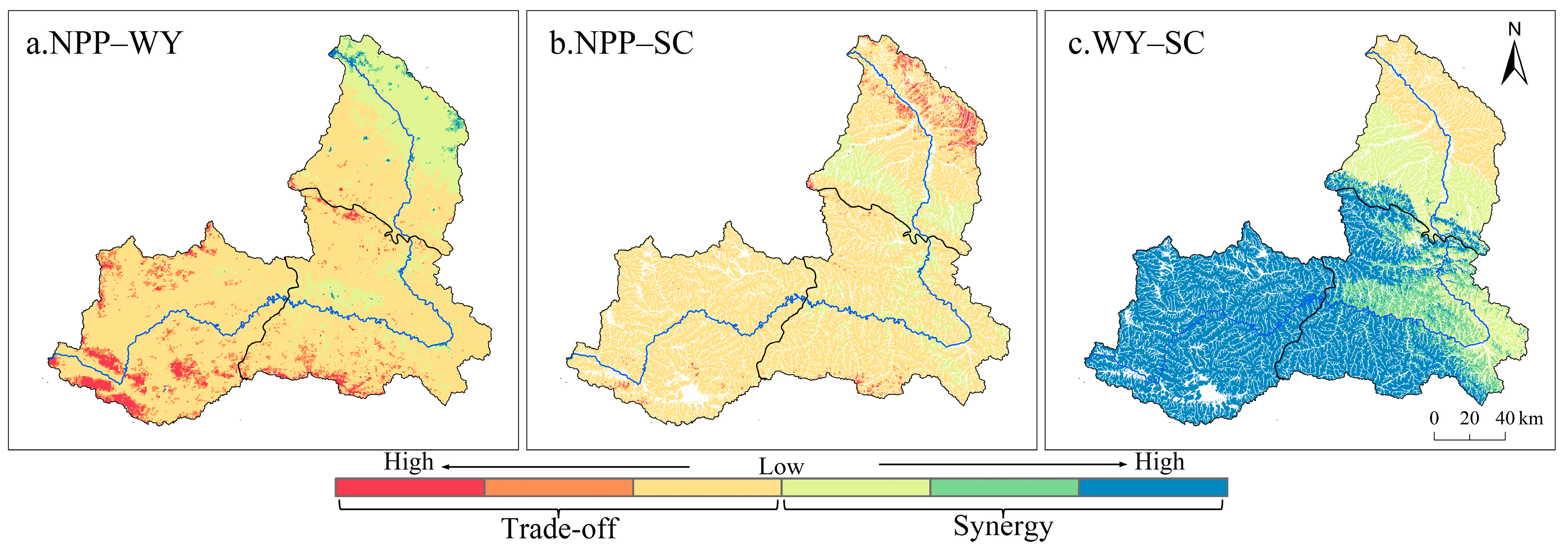
During 2000–2020, the relationship between the NPP, WY, and SC in the Taohe River Basin varied (Figure 3). The NPP–WY relationship was in a trade-off in the majority of its territory, with an area of 81.87%, with the areas showing a high trade-off being primarily distributed along the Xiqing Mountain; the area showing synergy was 18.13%, which was mainly distributed in the lower reaches of the cropping area. The NPP–SC relationship involved a trade-off that accounted for 87.20% of the area, with a small portion of the highly significant area distributed in the cropping area; the area in synergy accounted for 12.80% of the total area, with Taizi-Baishi Mountain making up the majority of that region. WY–SC were primarily in synergy, making up 88.43% of the area, of which the area in high synergy accounted for 59.86%, and was primarily distributed in the upper and middle reaches; only 11.57% of areas exhibit a trade-off, which shows a low trade-off, and was primarily located in the lower reaches of the cropping area. The extraction of the relationship between ESs and land use categories in 2020 reveals that cropland, forest, and grassland make up the majority of the total area. A noteworthy fact is that in the synergistic region of the NPP–SC, the area of cropland approached as much as 1217.7 km2 (Table 2).

3.3. Identification of Dominant Factors for Relationships between ESs

Using the factor detector of the geographical detector, the factors impacting how ESs interact with one another in the Taohe River Basin were identified (Table 3). Overall, natural rather than social factors better explained the relationships between ESs. In the natural factors, PRE, DEM, and NDVI had the strongest overall effects, with NPP–WY q-values of 0.45, 0.50, and 0.37, NPP–SC q-values of 0.21, 0.16, and 0.23, and WY–SC q-values of 0.71, 0.67 and 0.64, respectively. The social factors, POP and CROP, also had stronger effects on NPP–WY and WY–SC. Of these, POP had high q-values of 0.32 and 0.56 on NPP–WY and WY–SC, and CROP had q-values of 0.38 and 0.33 on NPP–WY and WY–SC. The interactions between the factors were investigated after the dominating factors had been determined (Figure 4). It discovered that all of the two-factor interactions had better explanatory power than a single-factor-driven impact and that the strength of the factor effects was significantly increased following the interaction.

3.4. Analysis of ESs Trade-Offs and Synergistic Impact Factors

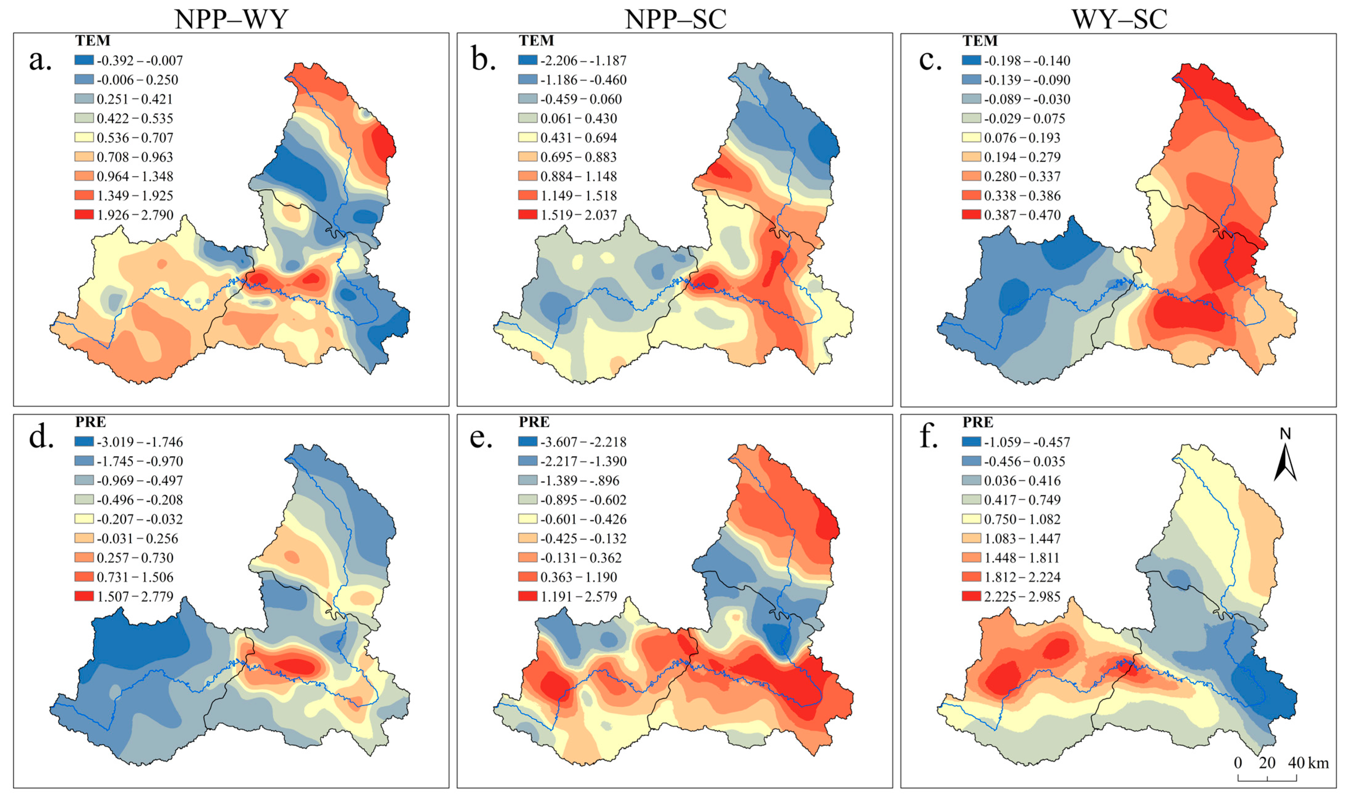
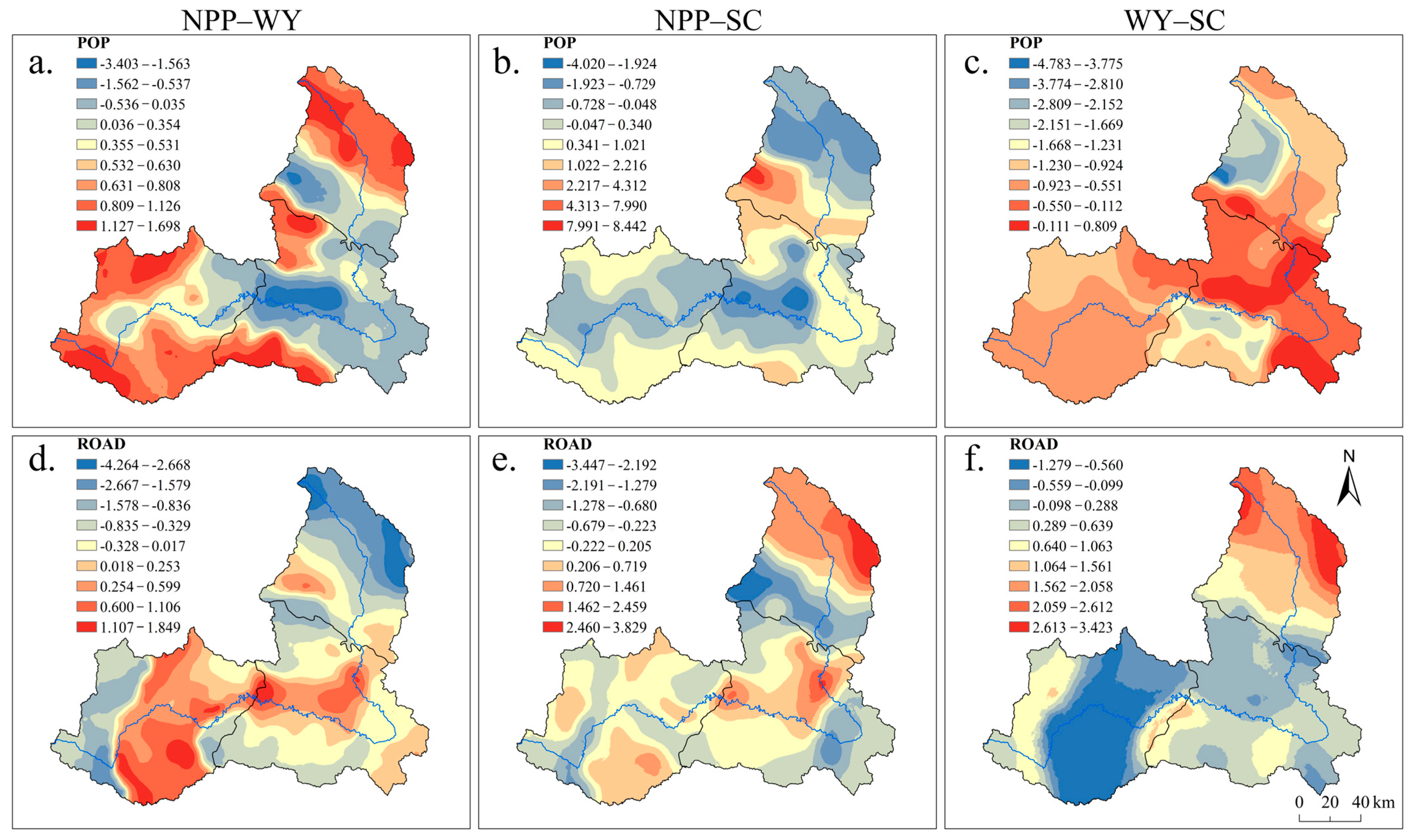
The selected impact factors were entered into GWR and MGWR, respectively; the closer the adjusted R2 value of the model was to 1, the lower the AICc value was, indicating a better fit of the model. The fitted parameters of both the GWR model and the MGWR model are better than the OLS model (Table 4). In addition, the variable bandwidth measures the spatial scale of action of each process and can reflect the difference in the scale of action of different impact factors on the relationship between ESs. A larger scale of action indicates less spatial heterogeneity in the effect of the impact factor, and conversely, more spatial heterogeneity [40]. By comparing the bandwidth of GWR and MGWR (Table 5), it can be seen that the bandwidths of variables in classical GWR are fixed, while based on the MGWR model, the bandwidths of variables take rich values and the scales of action of different variables vary greatly, which indicates that the MGWR model is better than the GWR model in terms of the fitting effect and can directly reflect the average of the differential scales of action of different variables, which is closer to the fitting effect of real values. Moreover, the R2 values of MGWR for NPP–WY, NPP–SC, and WY–SC were 0.813, 0.717, and 0.929, respectively, indicating that the results of the model were more reliable. Then, the simulation results were visualized through ArcGIS 10.7 software, and the distribution of regression coefficients of the inter-ES relationships and impact factors in the Taohe River Basin were obtained (Figure 5, Figure 6, Figure 7, Figure 8 and Figure 9). A positive regression coefficient suggests that the impact factor and ESs are positively correlated, and that this correlation will become more likely as the impact factor increases. Negative regression coefficients, on the other hand, demonstrate the opposite.

4. Discussion

4.1. Analysis of ESs Trade-Offs and Synergistic Features

Since 1998, several ecological restoration projects have been carried out, such as converting cropland back to forest (grass) and protecting natural forests; as a result, ESs have generally improved in the Taohe River Basin [41]. All three ESs displayed varying rates of growth, which is consistent with findings from earlier studies on the Tibetan Plateau and the Loess Plateau, where ESs exhibit erratic growth [42,43,44]. The Taohe River Basin is situated in a unique geographic region with a complicated topography. The soil in this kind of landscape depends on the extent of the vegetation’s root systems and their consequent ability to absorb water, preserve the structure of the soil, and reduce soil erosion [45]. However, high vegetation cover, robust transpiration, and water-trapping ability in the area may result in lower water production, particularly in the semi-arid Loess Plateau area [46,47].
This study uses bias correlation to quantify the relationship between ESs, and the findings indicate that NPP–WY and NPP–SC are primarily in a trade-off, while WY–SC are primarily in synergy. This result is consistent with Gong et al.’s (2019) [48] findings regarding the interaction between carbon storage (CS), WY, and SC in the Bailongjiang Watershed in southern Gansu. However, this is in contrast with the results of Niu et al. (2022) [44] for western China and Han et al. (2017) [49] for the three-rivers’ headwater region, where the ESs were all synergistic. This may be a result of regional variations in the local climate, geography, types of vegetation, and human activity [50,51].

4.2. Management Based on Trade-Offs and Synergies

The structure and support functions of ecosystems are impacted by human activity and climate change [52,53]. Examining how different natural and social factors affect how ESs interact may help in clarifying the detrimental effects of climate change and irresponsible human activity on ecosystems, developing sensible response policies, and successfully protecting the ecological environment. Using the results of the geographical detector and the simulation results of the MGWR model, the causes of the trade-offs and synergies between the three ESs are examined.
There are significant regional differences in the direction and magnitude of the response to each individual impact factor because different combinations of precipitation, temperature, and solar radiation have different effects on ESs in different regions and systems [54,55]. In areas in which the NPP, WY, and SC exhibit trade-offs in the upper and middle reaches, PRE is the primary factor altering this relationship (Figure 5). This is because precipitation is both a limiting factor for vegetation productivity and a significant recharge factor for flow production [56,57]. This is consistent with the conclusion of a study indicating that precipitation is the main factor affecting the growth of vegetation and the production of surface water [58]. It shows that precipitation is the primary factor influencing the development of the synergy between NPP and WY [59]. Planners can increase the amount of forest cover to produce shade and lessen water evaporation [54]. NPP–WY show synergistic cropping areas in the lower reaches, where the GDP, POP, and CROP are the main impact factors (Figure 7, Figure 8 and Figure 9). It has been demonstrated that the influence of human activity alters the trade-offs between ESs in the potential state and reveals synergies in the actual state [60]. It has also been suggested that increasing the intensity of human activity may increase the synergistic effects between ESs [24]. Similarly, in the lower regions in which NPP–SC showed high trade-offs, natural factors essentially encourage these trade-offs, whereas the GDP and POP obstruct this relationship (Figure 7 and Figure 8). As a result, the influence of human activity may have shifted the relationships between ESs. However, this does not imply that human activity has a beneficial effect on ESs, ROAD makes this type of trade-off possible (Figure 8). To simultaneously construct the ecological security pattern of the watershed, planners can coordinate the “three red lines” (ecological red line, red line for protecting arable land, and red line for urban development boundary) and improve multifunctional land use [61]. It is noteworthy that the left bank of the middle reaches of the Taohe River is a mixed area of pastoralism, forestry, and agriculture, and the impact of human activity on the local ecological environment is also greater. Thus, planners may take into account implementing strategies such as rotational grazing in sub-regions, lowering grazing to develop grasslands, and maintaining and protecting sizable areas under closure in ecologically vulnerable areas affected by human activity. In the Taizi-Baishi Mountain forest area, where NPP–SC are synergistic, the local vegetation cover is high, and it is the key area for natural forest protection projects in the watershed. Ecological conservation projects can improve vegetation and thus enhance the SC of a region, which in turn affects the trade-offs and synergies between SC and other ESs [59,62]. This synergy is a perfect illustration of the significant contribution ecological conservation projects make to local soil preservation and vegetation restoration. Localities should keep stepping up the implementation of local and national ecological construction policies, such as natural forest protection projects. The WY–SC relationship is mainly synergistic, and the PRE, DEM and NDVI are the main impact factors to promote this relationship (Figure 5 and Figure 6). This situation is more pronounced in the Die Mountain area with its large forest distribution in the middle reaches, as mountainous areas are sensitive to gradient changes in precipitation, vegetation cover, and elevation [55,63]. In contrast, the synergistic effect of GDP, POP, and CROP on Die Mountain is clearly negative (Figure 7, Figure 8 and Figure 9), which indicates that human activity may damage the local ecological environment and weaken the supply capacity of ESs [64]. Therefore, it is important to regulate human activity, reasonably coordinate ecological land use, and prioritize ecological protection; efforts to solve the problem of ecological protection and economic development are difficult to coordinate, and it is thus challenging to create a win–win situation of economic development and environmental friendliness. Furthermore, CROP and LU both significantly influenced the relationship between ESs (Figure 9), with the greater distance from cropland inhibiting this relationship in the majority of NPP–WY and NPP–SC regions. In regions where WY–SC acted as trade-offs, however, CROP and LU clearly supported trade-offs. The cause of this might be that excessive use of the land alters the physicochemical properties of the soil, which lowers soil productivity and harms ESs. Planners can, therefore, think about further optimizing the distribution of arable land resources and bolstering scientific and technological support based on strictly adhering to the red line of arable land.

4.3. Limitations and Perspectives

In this study, we concentrate on the trade-offs and synergies of ESs in the Taohe River Basin and the impact factors behind them from a spatial perspective. However, our study has some limitations: first, it is challenging to quantitatively explain the internal influence mechanisms that underlie trade-offs and synergies between ESs because these mechanisms are complex and different ESs respond to environmental variables and relationships in different ways. The effect of each impact factor on the relationship between ESs is usually the result of multiple impact factors acting together [65]. Furthermore, the impact factors chosen for this article are not all-inclusive; for instance, sunlight length, slope, slope orientation, and the percentage of built-up land can affect the trade-offs and synergies of ESs [11,54]. In the future, we should broaden the categories of impact factors and concentrate on examining how different impact factors interact to affect the relationship between ESs. Second, we looked at the trade-offs and synergies between ESs using just one scale. Yet, the interactions between ESs may be altered at various regional scales, and the response relationships may vary at other scales. The comparative study of ESs from multi-scale scales could be followed up. Third, this study is static and does not take into account that trade-offs and synergies may change over time. Therefore, future studies should focus on the dynamic evolutionary characteristics of ES interrelationships.

5. Conclusions

In this paper, three typical ESs in the Taohe River Basin from 2000 to 2020 were evaluated based on the CASA model and the InVEST model, and the relationships between different ESs were measured using the biased correlation method. Then, a geographic detector was selected to detect five natural factors and five social factors, and the regression coefficients of the trade-offs and synergies between ESs by impact factors were calculated using an MGWR model. Finally, a spatialized expression was performed to explore their spatial heterogeneity. The main research conclusions are as follows: (1) NPP, WY, and SC are increasing, averaging 488.99 gC/m2, 157.29 mm, and 1441.51 t/hm2 during a multi-year period in the Taohe River Basin; the high-value area of NPP, SC, and the low-value area of WY are concentrated in the region around Die Mountain and Taizi-Baishi Mountain, and the low-value NPP and SC regions were primarily found in the cropping areas in the lower Loess Plateau; (2) There are various relationships between NPP, WY, and SC; NPP–WY and NPP–SC are primarily trade-offs, whereas WY–SC is primarily synergistic. There is also a clear spatial distribution heterogeneity, with the biggest amount of cropland, forest, and grassland; (3) The effects of impact factors on the trade-offs and synergies between ESs exhibit spatial heterogeneity, and the distribution of PRE has a significant controlling effect on the spatial distribution of NPP and WY, where PRE was the primary factor affecting the trade-offs between NPP–WY and NPP–SC in the upper and middle reaches. GDP, POP, and CROP are the main factors affecting the NPP–WY synergy in the lower Loess Plateau cropland area; PRE, DEM, and CROP are the main impact factors affecting WY–SC synergy, and this influence is more obvious in the middle reaches of the Die Mountain forest area. Human activity has the potential to change the relationship between ESs.
This study can serve as a reference for research in other areas and advances our understanding of the synergy and trade-offs among ESs. To achieve sustainable development of the world’s ecological environment, it is advantageous to have a thorough grasp of the linkages between ecosystems. Future studies should concentrate on understanding the spatialization of relationships among various ESs and investigating the effects that dynamic and various spatial scales have on such relationships.

Author Contributions

Conceptualization, J.Z. and B.Z.; methodology, J.Z.; software, J.Z. and Y.Z.; resources, Y.S. and J.C.; data curation, Y.S. and X.Z.; writing—original draft preparation, J.Z.; writing—review and editing, J.Z. and B.Z.; supervision, B.Z. All authors have read and agreed to the published version of the manuscript.

Funding

This research was funded by the National Natural Science Foundation of China (NSFC), grant number 41561024.

Institutional Review Board Statement

Not applicable.

Informed Consent Statement

Not applicable.

Data Availability Statement

Not applicable.

Acknowledgments

We are very grateful to the editors and anonymous reviewers for their comments on the manuscript.

Conflicts of Interest

The authors declare no conflict of interest.

References

  1. Lévêque, C. Ecology: From Ecosystem to Biosphere; Science Publishers: Rawalpindi, Pakistan, 2003. [Google Scholar]
  2. Li, W.; Zhang, B.; Xie, G. Research on ecosystem services in China: Progress and perspectives. J. Nat. Resour. 2009, 24, 1–10. [Google Scholar]
  3. Assessment, M.E. Ecosystems and Human Well-Being: Wetlands and Water; World Resources Institute: Washington, DC, USA, 2005. [Google Scholar]
  4. Pereira, E.; Queiroz, C.; Pereira, H.M.; Vicente, L. Ecosystem services and human well-being: A participatory study in a mountain community in Portugal. Ecol. Soc. 2005, 10, 14. [Google Scholar] [CrossRef]
  5. Costanza, R.; d’Arge, R.; De Groot, R.; Farber, S.; Grasso, M.; Hannon, B.; Limburg, K.; Naeem, S.; O’neill, R.V.; Paruelo, J. The value of the world’s ecosystem services and natural capital. Nature 1997, 387, 253–260. [Google Scholar] [CrossRef]
  6. Busch, M.; La Notte, A.; Laporte, V.; Erhard, M. Potentials of quantitative and qualitative approaches to assessing ecosystem services. Ecol. Indic. 2012, 21, 89–103. [Google Scholar] [CrossRef]
  7. Howe, C.; Suich, H.; Vira, B.; Mace, G.M. Creating win-wins from trade-offs? Ecosystem services for human well-being: A meta-analysis of ecosystem service trade-offs and synergies in the real world. Glob. Environ. Chang. 2014, 28, 263–275. [Google Scholar] [CrossRef] [Green Version]
  8. Li, S.; Zhang, C.; Liu, J.; Zhu, W.; Ma, C.; Wang, J. The tradeoffs and synergies of ecosystem services: Research progress, development trend, and themes of geography. Geogr. Res. 2013, 32, 1379–1390. [Google Scholar]
  9. Pedrono, M.; Locatelli, B.; Ezzine-de-Blas, D.; Pesche, D.; Morand, S.; Binot, A. Impact of climate change on ecosystem services. In Climate Change and Agriculture Worldwide; Springer: Berlin/Heidelberg, Germany, 2016; pp. 251–261. [Google Scholar]
  10. Mooney, H.; Larigauderie, A.; Cesario, M.; Elmquist, T.; Hoegh-Guldberg, O.; Lavorel, S.; Mace, G.M.; Palmer, M.; Scholes, R.; Yahara, T. Biodiversity, climate change, and ecosystem services. Curr. Opin. Environ. Sustain. 2009, 1, 46–54. [Google Scholar] [CrossRef]
  11. Yang, S.; Zhao, W.; Liu, Y.; Wang, S.; Wang, J.; Zhai, R. Influence of land use change on the ecosystem service trade-offs in the ecological restoration area: Dynamics and scenarios in the Yanhe watershed, China. Sci. Total Environ. 2018, 644, 556–566. [Google Scholar] [CrossRef]
  12. Feng, Z.; Jin, X.; Chen, T.; Wu, J. Understanding trade-offs and synergies of ecosystem services to support the decision-making in the Beijing–Tianjin–Hebei region. Land Use Policy 2021, 106, 105446. [Google Scholar] [CrossRef]
  13. Cord, A.F.; Bartkowski, B.; Beckmann, M.; Dittrich, A.; Hermans-Neumann, K.; Kaim, A.; Lienhoop, N.; Locher-Krause, K.; Priess, J.; Schröter-Schlaack, C. Towards systematic analyses of ecosystem service trade-offs and synergies: Main concepts, methods and the road ahead. Ecosyst. Serv. 2017, 28, 264–272. [Google Scholar] [CrossRef]
  14. Dai, E.; Wang, X.; Zhu, J.; Zhao, D. Methods, tools and research framework of ecosystem service trade-offs. Geogr. Res. 2016, 35, 1005–1016. [Google Scholar]
  15. Shen, J.; Li, S.; Liang, Z.; Liu, L.; Li, D.; Wu, S. Exploring the heterogeneity and nonlinearity of trade-offs and synergies among ecosystem services bundles in the Beijing-Tianjin-Hebei urban agglomeration. Ecosyst. Serv. 2020, 43, 101103. [Google Scholar] [CrossRef]
  16. Ran, C.; Wang, S.; Bai, X.; Tan, Q.; Zhao, C.; Luo, X.; Chen, H.; Xi, H. Trade-offs and synergies of ecosystem services in southwestern China. Environ. Eng. Sci. 2020, 37, 669–678. [Google Scholar] [CrossRef]
  17. Shao, Y.; Xiao, Y.; Sang, W. Land use trade-offs and synergies based on temporal and spatial patterns of ecosystem services in South China. Ecol. Indic. 2022, 143, 109335. [Google Scholar] [CrossRef]
  18. Burkhard, B.; Kroll, F.; Nedkov, S.; Müller, F. Mapping ecosystem service supply, demand and budgets. Ecol. Indic. 2012, 21, 17–29. [Google Scholar] [CrossRef]
  19. Yang, X.; Zhou, Z.; Li, J.; Fu, X.; Mu, X.; Li, T. Trade-offs between carbon sequestration, soil retention and water yield in the Guanzhong-Tianshui Economic Region of China. J. Geogr. Sci. 2016, 26, 1449–1462. [Google Scholar] [CrossRef]
  20. Chen, T.; Huang, Q.; Wang, Q. Differentiation characteristics and driving factors of ecosystem services relationships in karst mountainous area based on geographic detector modeling: A case study of Guizhou Province. Acta Ecol. Sin. 2022, 42, 6959–6972. [Google Scholar]
  21. Nazeer, M.; Bilal, M. Evaluation of ordinary least square (OLS) and geographically weighted regression (GWR) for water quality monitoring: A case study for the estimation of salinity. J. Ocean Univ. China 2018, 17, 305–310. [Google Scholar] [CrossRef]
  22. Zhu, C.; Zhang, X.; Zhou, M.; He, S.; Gan, M.; Yang, L.; Wang, K. Impacts of urbanization and landscape pattern on habitat quality using OLS and GWR models in Hangzhou, China. Ecol. Indic. 2020, 117, 106654. [Google Scholar] [CrossRef]
  23. Mahara, D.O.; Fauzan, A. Impacts of Human Development Index and Percentage of Total Population on Poverty using OLS and GWR models in Central Java, Indonesia. EKSAKTA J. Sci. Data Anal. 2021, 2, 142–154. [Google Scholar] [CrossRef]
  24. Zhang, Z.; Liu, Y.; Wang, Y.; Liu, Y.; Zhang, Y.; Zhang, Y. What factors affect the synergy and tradeoff between ecosystem services, and how, from a geospatial perspective? J. Clean. Prod. 2020, 257, 120454. [Google Scholar] [CrossRef]
  25. Chen, J.; Wang, Y.; Sun, J.; Liang, E.; Shen, M.; Yang, B.; Jia, X.; Zhang, J. Precipitation dominants synergies and trade-offs among ecosystem services across the Qinghai-Tibet Plateau. Glob. Ecol. Conserv. 2021, 32, e01886. [Google Scholar] [CrossRef]
  26. Oshan, T.M.; Li, Z.; Kang, W.; Wolf, L.J.; Fotheringham, A.S. mgwr: A Python implementation of multiscale geographically weighted regression for investigating process spatial heterogeneity and scale. ISPRS Int. J. Geo-Inf. 2019, 8, 269. [Google Scholar] [CrossRef] [Green Version]
  27. Fathurahman, M.; Ratnasari, V. Geographically weighted multivariate logistic regression model and its application. Abstr. Appl. Anal. 2020, 2020, 8353481. [Google Scholar] [CrossRef]
  28. Yang, L.; Feng, Q.; Li, C.; Si, J.; Wen, X.; Yin, Z. Detecting climate variability impacts on reference and actual evapotranspiration in the Taohe River Basin, NW China. Hydrol. Res. 2017, 48, 596–612. [Google Scholar] [CrossRef] [Green Version]
  29. Liu, Z.; Chen, X.; Guan, X.; Shu, Z.; Yang, X.; Wang, G. Attribution of runoff change in the Taohe River Basin under a changing environment. Res. Soil Water Conserv. 2020, 27, 87–92+100. [Google Scholar]
  30. Li, C.; Yang, L.; Yang, W.; Wang, S. Land use and land cover change in Taohe River Basin and its driving forces. Sci. Geogr. Sin. 2014, 34, 848–855. [Google Scholar]
  31. Jianbing, W. Trend analysis for the variety of arid index in Taohe River basin in recent 40 years. Agric. Res. Arid Areas 2014, 32, 246–250. [Google Scholar]
  32. Wang, H.; Zhao, H. Dynamic changes of soil erosion in the taohe river basin using the RUSLE model and google earth engine. Water 2020, 12, 1293. [Google Scholar] [CrossRef]
  33. Li, C.; Wang, L.; Wanrui, W.; Qi, J.; Linshan, Y.; Zhang, Y.; Lei, W.; Cui, X.; Wang, P. An analytical approach to separate climate and human contributions to basin streamflow variability. J. Hydrol. 2018, 559, 30–42. [Google Scholar] [CrossRef]
  34. Cheng, L.; Wan, G.; Yang, M.; Wang, X.; Li, Y. The Runoff in the Upper Taohe River Basin and Its Responses to Climate Change. Water 2022, 14, 2094. [Google Scholar] [CrossRef]
  35. Zhu, L.; Liu, R.; Wen, J.; Zhao, M.; Wang, C. Climate change and drought evolution in the Tao River Basin in the past 50 years. J. Arid Meteorol. 2018, 36, 234–242. [Google Scholar]
  36. Li, C.; Wang, S.; Yang, L.; Yang, W.; Li, W. Spatial and temporal variation of meteorologica elementsin the Taohe River Basin from 1951 to 2010. J. Glaciol. Geocryol. 2013, 35, 1259–1266. [Google Scholar]
  37. Zhang, J.-S.; Kang, E.-S.; Lan, Y.-C.; Chen, R.-S.; Yao, J.-Z.; Pu, R.-F.; Chen, M.-X. Trend Analysis of the Precipitation and Runoff in the Taohe River Watershed during the Past 50 Years. J. Glaciol. Geocryol. 2003, 25, 72–82. [Google Scholar]
  38. Wang, S.; Li, C.; Yang, L. Drought trend analysis based on standardized precipitation index and the Z index in the Tao River Basin. Arid Zone Res. 2015, 32, 565–572. [Google Scholar]
  39. Zhou, F.-C.; Han, X.; Tang, S.; Song, X.; Wang, H. An improved model for evaluating ecosystem service values using land use/cover and vegetation parameters. J. Meteorol. Res. 2021, 35, 148–156. [Google Scholar] [CrossRef]
  40. Fotheringham, A.S.; Yang, W.; Kang, W. Multiscale geographically weighted regression (MGWR). Ann. Am. Assoc. Geogr. 2017, 107, 1247–1265. [Google Scholar] [CrossRef]
  41. Quanqin, S.; Jiangwen, F.; Jiyuan, L.; Fan, Y.; Hua, L.; Xiuchun, Y.; Mingxiang, X.; Peng, H.; Xingjian, G.; Lin, H. Approaches for monitoring and assessment of ecological benefits of national key ecological projects. Adv. Earth Sci. 2017, 32, 1174. [Google Scholar]
  42. Wang, S.; Jin, T.; Yan, L.; Gong, J. Ecosystem services trade-off and synergy change in the Ziwuling Region, Northwest China and their influencing factors. Chin. J. Appl. Ecol. 2022, 33, 3087–3096. [Google Scholar]
  43. Chen, X.; Wang, X.; Feng, X.; Zhang, X.; Luo, G. Ecosystem service trade-off and synergy on Qinghai-Tibet Plateau. Geogr. Res. 2021, 40, 18–34. [Google Scholar]
  44. Niu, L.; Shao, Q.; Ning, J.; Huang, H. Ecological changes and the tradeoff and synergy of ecosystem services in western China. J. Geogr. Sci. 2022, 32, 1059–1075. [Google Scholar] [CrossRef]
  45. Gyssels, G.; Poesen, J.; Bochet, E.; Li, Y. Impact of plant roots on the resistance of soils to erosion by water: A review. Prog. Phys. Geogr. 2005, 29, 189–217. [Google Scholar] [CrossRef] [Green Version]
  46. Sun, G.; Zhou, G.; Zhang, Z.; Wei, X.; McNulty, S.G.; Vose, J.M. Potential water yield reduction due to forestation across China. J. Hydrol. 2006, 328, 548–558. [Google Scholar] [CrossRef]
  47. Fu, Q.; Li, B.; Hou, Y.; Bi, X.; Zhang, X. Effects of land use and climate change on ecosystem services in Central Asia’s arid regions: A case study in Altay Prefecture, China. Sci. Total Environ. 2017, 607, 633–646. [Google Scholar] [CrossRef] [PubMed]
  48. Gong, J.; Liu, D.; Zhang, J.; Xie, Y.; Cao, E.; Li, H. Tradeoffs/synergies of multiple ecosystem services based on land use simulation in a mountain-basin area, western China. Ecol. Indic. 2019, 99, 283–293. [Google Scholar] [CrossRef]
  49. Han, Z.; Song, W.; Deng, X.; Xu, X. Trade-offs and synergies in ecosystem service within the three-rivers headwater region, China. Water 2017, 9, 588. [Google Scholar] [CrossRef] [Green Version]
  50. Sun, Y.; Liu, S.; Liu, Y.; Dong, Y.; Li, M.; An, Y.; Shi, F.; Beazley, R. Effects of the interaction among climate, terrain and human activities on biodiversity on the Qinghai-Tibet Plateau. Sci. Total Environ. 2021, 794, 148497. [Google Scholar] [CrossRef]
  51. He, J.; Shi, X.; Fu, Y. Identifying vegetation restoration effectiveness and driving factors on different micro-topographic types of hilly Loess Plateau: From the perspective of ecological resilience. J. Environ. Manag. 2021, 289, 112562. [Google Scholar] [CrossRef]
  52. Mahmoud, S.H.; Gan, T.Y. Impact of anthropogenic climate change and human activities on environment and ecosystem services in arid regions. Sci. Total Environ. 2018, 633, 1329–1344. [Google Scholar] [CrossRef]
  53. Desta, H.; Lemma, B.; Fetene, A. Aspects of climate change and its associated impacts on wetland ecosystem functions: A review. J. Am. Sci. 2012, 8, 582–596. [Google Scholar]
  54. Yang, M.; Gao, X.; Zhao, X.; Wu, P. Scale effect and spatially explicit drivers of interactions between ecosystem services—A case study from the Loess Plateau. Sci. Total Environ. 2021, 785, 147389. [Google Scholar] [CrossRef]
  55. Liu, L.; Wang, Z.; Wang, Y.; Zhang, Y.; Shen, J.; Qin, D.; Li, S. Trade-off analyses of multiple mountain ecosystem services along elevation, vegetation cover and precipitation gradients: A case study in the Taihang Mountains. Ecol. Indic. 2019, 103, 94–104. [Google Scholar] [CrossRef]
  56. Zuazo, V.H.D.; Pleguezuelo, C.R.R. Soil-erosion and runoff prevention by plant covers: A review. Sustain. Agric. 2009, 28, 785–811. [Google Scholar]
  57. Fatichi, S.; Ivanov, V.Y. Interannual variability of evapotranspiration and vegetation productivity. Water Resour. Res. 2014, 50, 3275–3294. [Google Scholar] [CrossRef]
  58. Whitehead, P.G.; Wilby, R.L.; Battarbee, R.W.; Kernan, M.; Wade, A.J. A review of the potential impacts of climate change on surface water quality. Hydrol. Sci. J. 2009, 54, 101–123. [Google Scholar] [CrossRef] [Green Version]
  59. Ma, S.; Wang, L.-J.; Jiang, J.; Chu, L.; Zhang, J.-C. Threshold effect of ecosystem services in response to climate change and vegetation coverage change in the Qinghai-Tibet Plateau ecological shelter. J. Clean. Prod. 2021, 318, 128592. [Google Scholar] [CrossRef]
  60. Zhao, T.; Pan, J.; Bi, F. Can human activities enhance the trade-off intensity of ecosystem services in arid inland river basins? Taking the Taolai River asin as an example. Sci. Total Environ. 2023, 861, 160662. [Google Scholar] [CrossRef]
  61. Qian, C.; Gong, J.; Zhang, J.; Liu, D.; Ma, X. Change and tradeoffs-synergies analysis on watershed ecosystem services: A case study of Bailongjiang Watershed, Gansu. Acta Geogr. Sin. 2018, 73, 868–879. [Google Scholar]
  62. Wang, Y.; Dai, E. Spatial-temporal changes in ecosystem services and the trade-off relationship in mountain regions: A case study of Hengduan Mountain region in Southwest China. J. Clean. Prod. 2020, 264, 121573. [Google Scholar] [CrossRef]
  63. Yu, Y.; Li, J.; Zhou, Z.; Ma, X.; Zhang, X. Response of multiple mountain ecosystem services on environmental gradients: How to respond, and where should be priority conservation? J. Clean. Prod. 2021, 278, 123264. [Google Scholar] [CrossRef]
  64. Li, W.; Zhao, X.; Du, Y.; Ma, P. Spatio-temporal changes of the coupling relationship between ecosystem services and residents’ well-being in Qinba. J. Nat. Resour. 2021, 36, 2522–2540. [Google Scholar] [CrossRef]
  65. Feng, Q.; Zhao, W.; Fu, B.; Ding, J.; Wang, S. Ecosystem service trade-offs and their influencing factors: A case study in the Loess Plateau of China. Sci. Total Environ. 2017, 607, 1250–1263. [Google Scholar] [CrossRef] [PubMed]
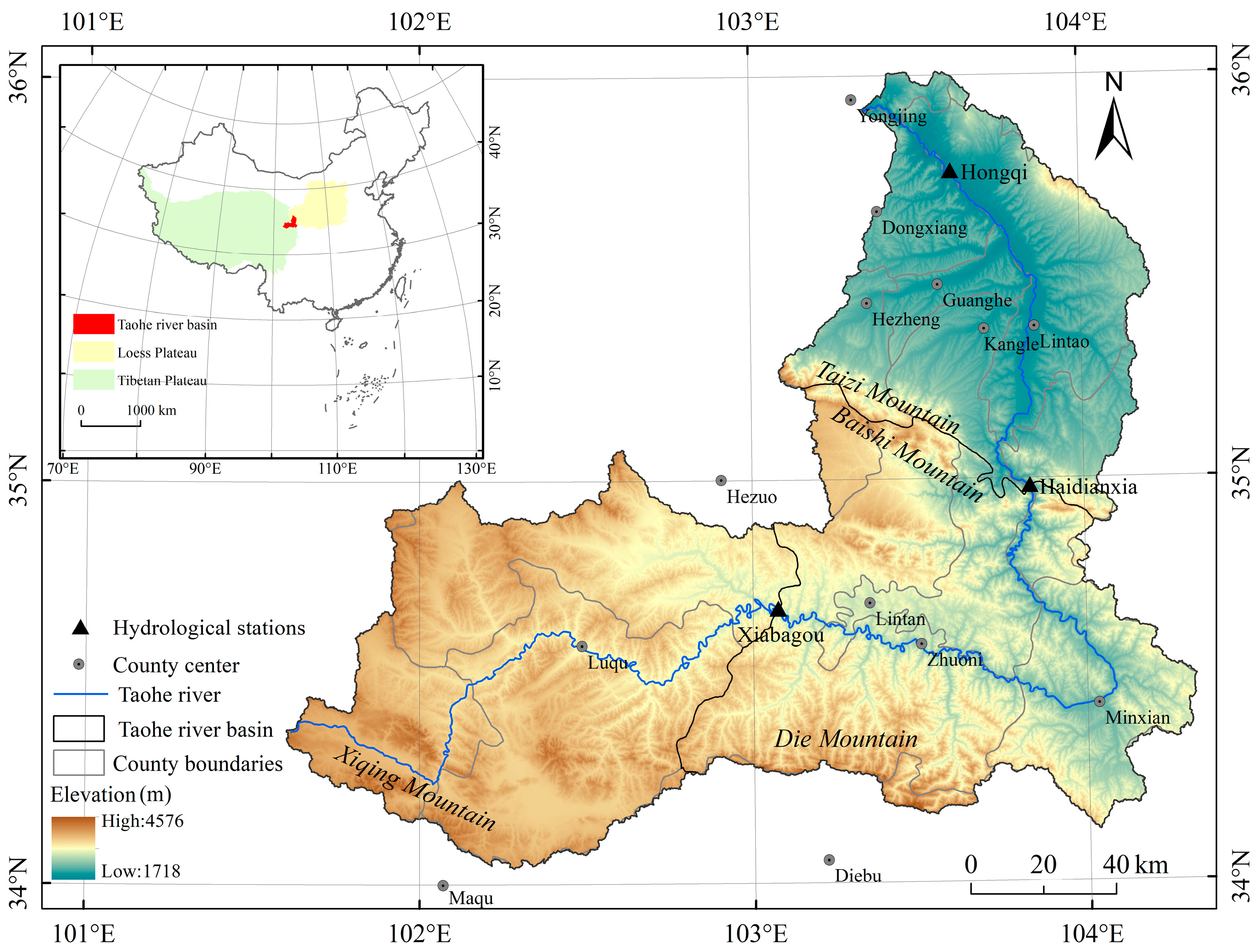
Figure 1. Location of the study area.
Sustainability 15 09689 g001
Figure 2. Spatial distribution of ESs in the Taohe river basin.
Sustainability 15 09689 g002
Figure 3. Spatial distribution of ES trade-offs and synergies in 2000–2020.
Sustainability 15 09689 g003
Figure 4. The interaction of impact factors on the trade-offs and synergies between ESs.
Sustainability 15 09689 g004
Figure 5. Spatial variation in TEM and PRE regression coefficients in MGWR. (ac) indicate the spatial variation of regression coefficients of TEM with NPP–WY, NPP–SC and WY–SC, respectively; (df) indicate the spatial variation of regression coefficients of PRE with NPP–WY, NPP–SC and WY–SC, respectively.
Sustainability 15 09689 g005
Figure 6. Spatial variation in DEM and NDVI regression coefficients in MGWR. (ac) indicate the spatial variation of regression coefficients of DEM with NPP–WY, NPP–SC and WY–SC, respectively; (df) indicate the spatial variation of regression coefficients of NDVI with NPP–WY, NPP–SC and WY–SC, respectively.
Sustainability 15 09689 g006
Figure 7. Spatial variation in SOIL and GDP regression coefficients in MGWR. (ac) indicate the spatial variation of regression coefficients of SOIL with NPP–WY, NPP–SC and WY–SC, respectively; (df) indicate the spatial variation of regression coefficients of GDP with NPP–WY, NPP–SC and WY–SC, respectively.
Sustainability 15 09689 g007
Figure 8. Spatial variation in POP and ROAD regression coefficients in MGWR. (ac) indicate the spatial variation of regression coefficients of POP with NPP–WY, NPP–SC and WY–SC, respectively; (df) indicate the spatial variation of regression coefficients of ROAD with NPP–WY, NPP–SC and WY–SC, respectively.
Sustainability 15 09689 g008
Figure 9. Spatial variation in CROP and LU regression coefficients in MGWR. (ac) indicate the spatial variation of regression coefficients of CROP with NPP–WY, NPP–SC and WY–SC, respectively; (df) indicate the spatial variation of regression coefficients of LU with NPP–WY, NPP–SC and WY–SC, respectively.
Sustainability 15 09689 g009
Table 1. Calculation methods for ESs.
ESsModelsMathematical Algorithms
NPPCASA N P P ( x , t ) = A P A R ( x , t ) × ε ( x , t )
N P P ( x , t ) : net primary productivity of vegetation at a time t for pixels x (gC/m2); A P A R ( x , t ) : photosynthetically active radiation absorbed by pixels x at a time t (MJ/m2); ε ( x , t ) : actual light energy utilization at a time t for pixels x (gC/MJ).
WYWater yield module of InVEST Y ( x ) = 1 A E T ( x ) P ( x ) × P ( x )
Y ( x ) : annual water yield of the pixels x (mm); A E T ( x ) : actual annual evapotranspiration of the pixels x (mm); P ( x ) : annual precipitation of the pixels x (mm).
SCSediment retention module of InVEST R K L S = R × K × L S  
U S L E = R × K × L S × C × P
  S C = R K L S U S L E
S C : soil conservation amount (t/hm2); R K L S : potential soil erosion amount (t/hm2); U S L E : actual soil erosion amount under ecological management measures (t/hm2); R , K , L S , C and P indicate rainfall erosion factor, soil erosion factor, slope length slope factor, vegetation cover and management factor, and measure factor of soil and water conservation, respectively.
Table 2. ESs trade-offs and synergistic areas for different land use types in 2020 (unit: km2).
CroplandForestGrasslandShrubsWaterBareConstructed Land Total
NPP–WYTrade-off3791.522596.8613,888.49371.525.851.087.2920,662.61
Synergy1698.75370.622410.7448.0642.30.094.774575.33
NPP–SCTrade-off2812.142062.7111,699.79287.463.511.081.4416,868.13
Synergy1217.7315.27875.5259.497.92002475.9
WY–SCTrade-off843.750.181387.620.271.350.0902233.26
Synergy3185.552377.811,187.36346.6810.080.990.7217,109.18
Table 3. Individual impact factors’ detection of the trade-offs and synergies between ESs.
Natural FactorsSocial Factors
TEMPREDEMNDVISOILGDPPOPROADCROPLU
NPP–WY0.480.450.500.370.160.180.320.040.380.06
NPP–SC0.160.210.160.230.120.040.040.010.070.07
WY–SC0.590.710.670.640.110.310.560.170.330.31
Notes: all of the above values passed the significance test at p = 0.05.
Table 4. Model simulation results of the relationship between ESs and impact factors in MGWR.
OLSGWRMGWR
RSSR2AICcRSSR2AICcRSSR2AICc
NPP–WY512.5950.6552662.534253.1960.8091975.825256.3510.8131882.806
NPP–SC845.9080.4313411.415379.2300.7042697.604423.1760.7172632.314
WY–SC241.1300.8381535.07882.7870.935457.18496.1430.929457.845
Notes: the total number of samples was 1495.
Table 5. Bandwidth of GWR and MGWR.
NPP–WYNPP–SCWY–SC
GWRMGWRGWRMGWRGWRMGWR
TEM1574312343116119
PRE157541234811643
DEM157431234311643
NDVI15766123118116244
SOIL157284123154116661
GDP1576612371116324
POP157431234311643
ROAD157581234311643
CROP15711512335711670
LU15735412389911659
Disclaimer/Publisher’s Note: The statements, opinions and data contained in all publications are solely those of the individual author(s) and contributor(s) and not of MDPI and/or the editor(s). MDPI and/or the editor(s) disclaim responsibility for any injury to people or property resulting from any ideas, methods, instructions or products referred to in the content.