Integration of UAV and GF-2 Optical Data for Estimating Aboveground Biomass in Spruce Plantations in Qinghai, China

Abstract

More refined and economical aboveground biomass (AGB) monitoring techniques are needed because of the growing significance of spruce plantations in climate change mitigation programs. Due to the challenges of conducting field surveys, such as the potential inaccessibility and high cost, this study proposes a convenient and efficient alternative to traditional field surveys that integrates Gaofen-2 (GF-2) satellite optical images and unmanned aerial vehicle (UAV)-acquired optical and point cloud data to provide a reliable and refined estimation of the aboveground biomass (AGB) in spruce plantations. The feasibility of using data produced from the semiautomatic processing of UAV-based images and photogrammetric point clouds to replace conventional field surveys of sample plots in a young spruce plantation was evaluated. The AGB in 53 sample plots was estimated using data extracted from the UAV imagery. The UAV plot data and GF-2 optical data were used in four regression models to estimate the AGB in the study area. The coefficient of determination (R²), root-mean-square error (RMSE), mean percent standard error (MPSE), and Lin’s concordance correlation coefficient (LCCC) were calculated through five-fold cross-validation and stratified random sampling to evaluate the models’ efficacies. In the end, the most accurate model was used to generate the spatial distribution map of the AGB. The results revealed the following: (1) the individual-tree height (R² = 0.90) and crown diameter (R² = 0.74) extracted from UAV data were accurate enough to replace field surveys used to obtain the AGB at the plot levels; (2) the random forest (RF) model (R² = 0.86; RMSE = 1.75 t/ha; MPSE = 15.75%; LCCC = 0.91) outperformed the ordinary least-squares (OLS) model (R² = 0.68; RMSE = 2.49 t/ha; MPSE = 22.94%; LCCC = 0.81), artificial neural network (ANN) model (R² = 0.67; RMSE = 2.54 t/ha; MPSE = 21.48%; LCCC = 0.80), and support vector machine (SVM) model (R² = 0.60; RMSE = 2.84 t/ha; MPSE = 31.73%; LCCC = 0.76) in terms of the estimation accuracy; (3) an AGB map generated by the random forest model was in good agreement with field surveys and the age of the spruce plantations. Therefore, the method proposed in this study can be used as a refined and cost-effective way to estimate the AGB in young spruce plantations.

1. Introduction

Carbon sinks refer to the process of mitigating climate change by absorbing greenhouse gases, and approximately 50% of human-caused CO₂ emissions are removed from the atmosphere each year by ocean and land ecosystems [1]. In terrestrial ecosystems, forests have the largest carbon stock, contributing about 80% of the aboveground biomass (AGB) carbon and 40% of the belowground biomass carbon. This means that forests are responsible for most of the world’s carbon storage [2]. Therefore, forests play a crucial role in regulating the global carbon cycle and slowing global climate change. Thus, there has been an increase in studies examining carbon stocks in forests [2,3]. According to the ninth forest inventory report (2014–2018), China’s forest area is 220 million km², of which 80 million km² is plantation forests, accounting for 36% of the total forest area [4]. Plantation forests are also the subject of several international forestry carbon sink transactions, including the verified carbon standard (VCS), Gold Standard (GS), and Chinese Certified Emission Reduction (CCER) [5]. However, carbon sink measurement methods for plantation forests require improvements, especially for young forests. Spruce is an important tree species used for afforestation and reforestation projects in the southwestern Qilian Mountains in Qinghai Province, China [6]. Timely information on the growth status of planted spruce forests is crucial for monitoring changes in their carbon stocks.

AGB is a critical characteristic of forest ecosystems and reflects their productivity [7]. With regard to planted spruce forests in the southwestern Qilian Mountains in Qinghai Province, previous studies have mostly used traditional field surveys to estimate their AGB [8,9,10]. Traditional field survey approaches may be precise and offer thorough information on forest structure and composition [11]. However, they are inefficient, laborious, and hard to replicate widely in inaccessible or remote areas [12]. Therefore, after using the traditional method to determine the allometric equation of planted spruce forests [13], we explored a more convenient and economical method that can be used to measure its AGB over a large area. Remote sensing can minimize human, material, resource, and environmental constraints because it has the advantage of macroscopic and dynamic monitoring [14]. Remote sensing data from various sources have been used in many studies to estimate aboveground biomass (AGB). Low-resolution optical data, such as MODIS [15], have been widely used for the large-scale continuous estimation of forest biomass. For example, Baccini et al. estimated the aboveground biomass across the entirety of tropical Africa using MODIS data with a resolution of 1 km [16]. Medium-resolution optical data, such as Landsat, can better reflect information on the forest ecosystem composition, community structure, and tree species distribution. Landsat provides long-term, continuous, and free multispectral remote sensing data and is one of the primary data sources for estimating forest biomass. Various variables related to forest biomass can be extracted from Landsat data. Zhu et al. found that the correlation between the autumn NDVI and forest biomass was stronger in their study area when using Landsat images to estimate forest biomass [17]. High-resolution optical data, such as those obtained from Gaofen-2 (GF-2), can provide detailed spatial information and extract texture features of forest areas. Gou et al. found that incorporating texture features improved the accuracy of forest biomass estimation when using GF-2 data [18]. Extremely high-resolution optical remote sensing images are generally used to extract individual-tree structure information for estimating the tree-level AGB and then obtaining the forest AGB [19]. Jones et al. used RGB images obtained from UAVs to extract individual-tree parameters and estimate the AGB of mangroves [20]. In particular, high-resolution images are suitable for estimating the AGB in plantation forests, which are often not continuous and may have varying vegetation densities. These images also provide sufficient coverage for regional-scale AGB estimation [18,21,22]. The relationship between forest-related remote sensing parameters and AGB is often nonlinear, leading to the considerable use of nonparametric models in AGB estimation [23,24,25,26]. Machine learning algorithms, such as random forests (RFs), support vector regression (SVR), artificial neural networks (ANNs), and k-nearest neighbors (k-NNs), have been applied due to their effective handling of enormous datasets and the relative simplicity with which they can simulate complicated nonlinear interactions between variables [27]. ANNs can effectively solve the problems of nonlinearity, non-Gaussianity, and noise in the data, even if there is a conflicting relationship between the response variable and explanatory variables. However, they require large datasets to obtain reliable certainty in biomass estimation [25]. The RF model is commonly used to handle small-sample AGB estimation in forest applications, indicating its suitability for estimating the AGB in the young spruce plantations of our study area [22].

Airborne laser scanning (ALS)-like 3D point clouds and digital surface models (DSMs) can now be easily generated thanks to advancements in hardware and photogrammetric algorithms, including dense image matching (DIM) and structure from motion (SfM) [28,29]. For open-canopy forests (e.g., young plantations), a digital elevation model (DEM) can also be generated from DSMs or point clouds [30]. Accurate DSMs and DEMs are a prerequisite for obtaining the structural parameters of trees [31]. On the one hand, UAV data are often combined with other data to improve the accuracy of forest AGB estimation. For instance, Zhu et al. incorporated a UAV-derived digital surface model (DSM) into GF data, which effectively improved the accuracy of mangrove AGB estimation [22]. However, such an approach still requires field surveys to obtain the plot-level AGB. On the other hand, some studies have utilized UAV data to estimate the AGB at the individual-tree level, thereby obtaining the forest-level AGB [20]. The process of individual tree crown delineation (ITCD) serves as a prerequisite for estimating the AGB at the individual-tree level using UAV data [32]. For airborne laser scanning (ALS) data, the prevalent approach involves an initial detection of treetops using local maxima (LM), followed by the delineation of tree crowns through the region-growing or watershed segmentation methods [33]. In the context of aerial imagery, the commonly employed methods for ITCD include valley following, region growing, and watershed segmentation. The essence of these methods lies in identifying the threshold that distinguishes tree crowns from the background, thereby facilitating ITCD [34]. These methods primarily consider the spectral information of the individual tree crowns, while lacking information on the vertical structure of the canopy [35]. Although this limitation makes ITCD challenging for general forests, these methods are sufficient for delineating individual tree crowns in open-canopy forests within a monoculture [36,37]. UAVs have rapidly become a popular option for measuring and mapping ecosystems [38]. However, due to the limitations of UAVs, this method is often difficult to apply over larger areas for AGB estimation. Therefore, in this study, we aimed to take advantage of the low-cost and vegetation-parameter-extraction capabilities of UAV-derived DIM-based point clouds at a centimeter-level resolution to replace field surveys for AGB estimation [39]. We further aimed to integrate this method with satellite remote sensing data to monitor the forest AGB over larger areas.

This research proposes a new approach for quantifying the AGB of huge regions of young spruce plantations using photogrammetry-based point clouds instead of traditional field sampling methods, and by using wall-to-wall GF-2 data as the input feature parameters in the optimal model for AGB estimation and mapping. The objectives of this study are to (1) assess the efficacy of UAV-derived vegetation indices (VIs) and photogrammetric point clouds in measuring individual tree crown diameters and heights, (2) explore the applicability of GF-2 MSI-derived indicators to predict the AGB of young spruce plantations, and (3) compare the accuracies of AGB estimates from different models. The proposed AGB monitoring method applies to climate change studies to enhance CO₂ sequestration in the alpine regions of northwest China.

2. Materials and Methods

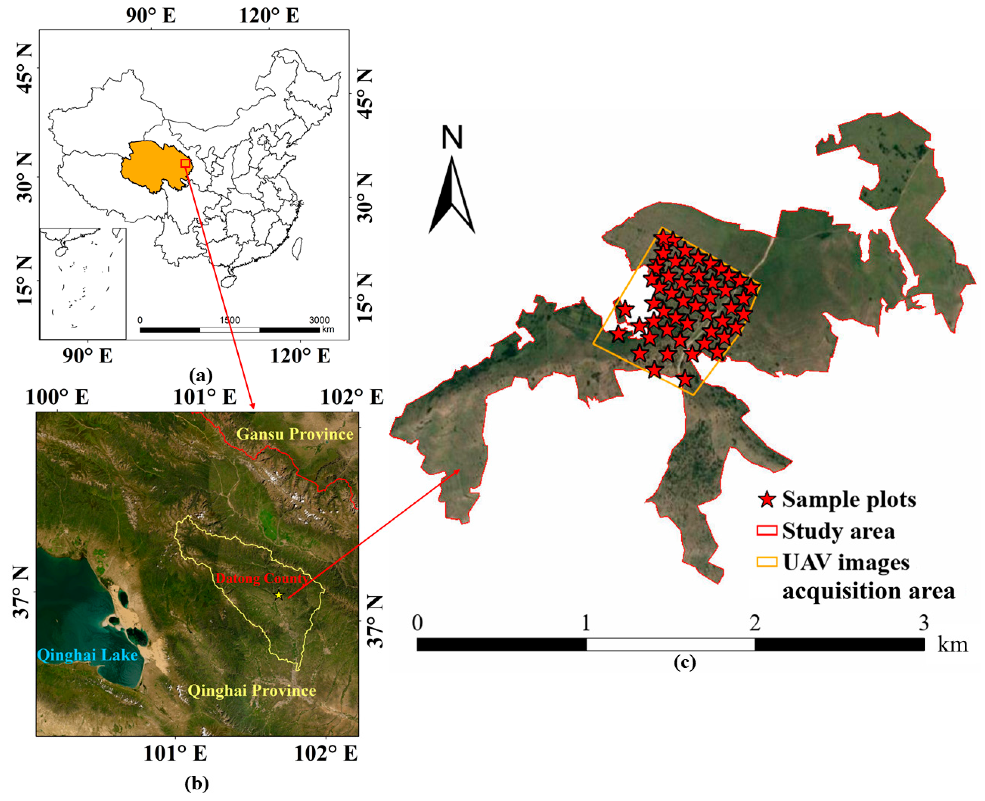
2.1. Study Area

This study was conducted on spruce plantations in Datong County, Xining City, Qinghai Province, China (37°5′22″–37°6′34″ N; 101°35′8″–101°37′1″ E), located in the southwestern Qilian Mountains, which is a transition zone from the Loess Plateau to the Qinghai–Tibetan Plateau (Figure 1). The study area was located at a 174.78 ha afforestation project planted between 2004 and 2014. The native forest type in the study area is mainly pure spruce forest; thus, Picea crassifolia was planted at a density of 2200 trees/ha [40].

The study area has a highland continental climate with an average air temperature ranging from −6 °C to 5.2 °C and annual precipitation ranging from 450 to 820 mm [41]. We selected spruce plantations with trees aged 7–17 years because the objective was to evaluate the potential for carbon sink trading, which is not possible in older forests. The plantations are located at 2940–3070 m above sea level. They exhibit good productivity, with a few dead branches or standing dead trees. This study area is representative of the Qinghai afforestation project.

2.2. Satellite Data: Acquisition and Preprocessing

Launched by the China National Space Administration (CNSA) in Taiyuan, China, in August 2014, GF-2 is capable of capturing high-resolution images. The data are widely used in surveys of land usage, mineral resources, and forest resources [42]. One panchromatic band with 0.8 m resolution and four multispectral bands with 3.2 m resolution—blue (B), green (G), red (R), and near-infrared (NIR) resolution—make up the GF-2 image. The GF-2 multispectral image used in this study was acquired from the Land Observing Satellite Data Service platform and shot on 11 September 2021.

The GF-2 images were preprocessed using the ENVI 5.3.1 software, which included radiometric calibration, atmospheric correction, and geometric correction. We used the fast line-of-sight atmospheric analysis of the spectral hypercubes (FLAASH) tool in the ENVI software for the atmospheric correction of the images. Additionally, we geo-corrected the images using ground control points (GCPs) and a 1:10,000 topographic map to ensure the images were not off by more than 0.5 pixels.

Then, we calculated eight VIs—the difference vegetation index (DVI); enhanced vegetation index (EVI); green normalized difference vegetation index (GNDVI); modified soil-adjusted vegetation index (MSAVI); normalized difference vegetation index (NDVI); ratio vegetation index (RVI); soil-adjusted vegetation index (SAVI); and transformed soil-adjusted vegetation index (TSAVI)—using the images. We also calculated 8 texture features for each of the 4 bands (window size: 3 × 3; direction: [1, 1]). As inputs to the models, the multispectral images, VIs, and texture features were utilized to estimate the AGB of the spruce plantation (

Table 1. Multispectral bands, vegetation indices, and texture features of GF-2 images used in this study.

Predictor Variable	Band/Index	Definition
Multispectral bands	B1	Blue, 450–520 nm
	B2	Green, 520–590 nm
	B3	Red, 630–690 nm
	B4	Near-infrared (NIR), 760–890 nm
Vegetation indices	DVI	B4 − B3
	EVI	2.5 × [(B4 − B3)/(B4 + 6 × B3 − 7.5 × B1 + 1)]
	GNDVI	(B4 − B2)/(B4 + B2)
	MSAVI	0.5 × [2 × B4 + 1 − $\sqrt{{\left(2\times \mathrm{B}4+1\right)}^2-8\times \left(\mathrm{B}4-\mathrm{B}3\right)}$]
	NDVI	(B4 − B3)/(B4 + B3)
	RVI	B4/B3
	SAVI	1.5 × (B4 − B3)/(B4 + B3 + 0.5)
	TSAVI	(0.33 × (B4 − 0.33 × B3 − 0.5))/(0.5 × B4 + B3 − 0.5 × 0.33 + 1.5 × (1 + 0.332))
Texture features	Mean	${\displaystyle \sum _{ij=0}^{N-1}}i{P}_{ij}$
	Variance	${\displaystyle \sum _{ij=0}^{N-1}}{P}_{ij}\times (i-mean{)}^2$
	Entropy	${\displaystyle \sum _{ij=0}^{N-1}}{P}_{ij}\times (-\mathrm{l}\mathrm{n}{P}_{ij})$
	Second moment	${\displaystyle \sum _{ij=0}^{N-1}}{P}_{ij}^2$
	Correlation	${\displaystyle \sum _{ij=0}^{N-1}}{P}_{ij}\left[\frac{(i-mean)-(j-mean)}{\sqrt{varianc{e}_i\times varianc{e}_j}}\right]$
	Homogeneity	${\displaystyle \sum _{ij=0}^{N-1}}i\frac{P_i}{1+(i-j{)}^2}$
	Contrast	${\displaystyle \sum _{ij=0}^{N-1}}i{P}_{ij}\times (i-j{)}^2$
	Dissimilarity	${\displaystyle \sum _{ij=0}^{N-1}}i{P}_{ij}\times |i-j|$

DVI: difference vegetation index; EVI: enhanced vegetation index; GNDVI: green normalized difference vegetation index; MSAVI: modified soil-adjusted vegetation index; NDVI: normalized difference vegetation index; RVI: ratio vegetation index; SAVI: soil-adjusted vegetation index; TSAVI: transformed soil-adjusted vegetation index; $P_{ij}$: normalized co-occurrence matrix.

).

2.3. Sampling Data Collection and Processing

Before the field investigation, a total of 53 sample plots, 5 × 5 m, were selected in the core area of the spruce plantation using Google Earth to ensure that each sample plot contained tree information within only 1 pixel size of the GF-2 image for a more refined AGB estimation. These sample plots contained spruce trees in various growth conditions to ensure sufficient sample variability to establish the AGB estimation model. To compare and validate field and UAV-based measurements, the crown diameters and tree heights of 97 trees were measured within 53 sample plots during our field survey (from 1 to 3 trees per plot). The measured trees were marked with red cloths before the UAV flight so that they could be found in the resulting orthomosaic maps. The crown diameters and tree heights were extracted from the derived vegetation indices and photogrammetric point clouds.

We conducted both aerial UAV photography and field measurements in September 2021. The multispectral images were acquired using a DJI Phantom 4 Multispectral (P4M), which is equipped with a real-time kinematic (RTK) GNSS system, an inertial measurement unit (IMU), a barometer, and a compass. Furthermore, to enhance the georeferencing accuracy of the UAV images, DJI RTK-2 GNSS base equipment was utilized, with a horizontal positioning accuracy of 0.02 m and a vertical positioning accuracy of 0.03 m. Additionally, a six-camera, two-million-pixel, multispectral sensor was equipped in the DJI-P4M UAV. It can capture images in the blue (450 nm ± 16 nm), green (560 nm ± 16 nm), red (650 nm ± 16 nm), red-edge (RE) (730 nm ± 16 nm), near-infrared (840 nm ± 26 nm), and visible-light (RGB) spectra. The flight height was 189 m, and the speed was 8 m/s. The image overlap and sidelap were 80% to facilitate the creation of 3D information. At this altitude and speed and these overlap settings, the spatial resolution was 10 cm. On a sunny day without clouds, the flight mission was conducted between 10:00 and 14:00. Images of the reference reflectance panel were obtained for calibration before the flight. After the flight, we used DJI Terra 3.4.4 software to calibrate the multispectral images and process them into orthomosaic maps for individual-tree-canopy extraction.

First, we cropped the images to match the spatial size of the sample plots (i.e., a rectangle with a side length of 5 m). Second, several VIs, such as the NDVI and EVI, were calculated for each sample plot, and we extracted the tree crowns using the OTSU threshold segmentation method. OTSU is an algorithm designed to determine the threshold for the binary segmentation of images, also known as the maximum inter-class variance method. This method capitalizes on the grayscale characteristics of the image, dividing it into two components: the background and the foreground. At this point of division, the inter-class variance between the foreground and background images is maximized, implying a minimized probability of misclassification [43]. In this study, the OTSU method was tested and proven effective at extracting tree crowns from the background. We compared the tree extraction for different VIs and found that the EVI produced the best results. The threshold segmentation results were vectorized, and the minimum boundary geometry tool was used to obtain the minimum outer circle of the tree crown. The geometric features of these circles were calculated to obtain the crown diameters of the individual trees. The vector boundaries of the individual trees were used for the subsequent tree height extraction.

The UAV aerial photography data were reprocessed into a DIM point cloud using the Pix4Dmapper 4.5.6 software. Aligning images and generating a georeferenced sparse point cloud are two of Pix4Dmapper’s main functions, and both are accomplished using proprietary algorithms based on SfM and stereo-matching methods. The sky was automatically deleted from DJI Phantom 4 drone images during the image alignment process in Pix4Dmapper. When this was complete, multi-view stereo-reconstruction methods were used to densify the point cloud. In this study, the original image size and high-density point settings were used to make point clouds that were denser than the default settings. Even if no additional GCPs were collected to improve the accuracy, the data collected by the DJI Phantom 4 drone had high accuracy because the drone used real-time kinematic (RTK) positioning, meeting the experimental requirements.

LiDAR360 software’s Remove Outliers and Noise Filter tools were used to filter the noise points above and below the spruce plantation. Subsequently, the ground point classification tool in the LiDAR360 software was used to sort the points into ground points and nonground points. These ground points were further checked and edited manually to produce a DEM with a resolution of 0.1 × 0.1 m. A DSM with a resolution of 0.1 × 0.1 m was also produced based on all point clouds. After, we subtracted the DEM heights from the DSM heights for each sample plot to obtain a canopy height model (CHM) with a resolution of 0.1 × 0.1 m.

Trees were only selected for the study if at least half of their crown surface was located inside the plots. To prevent accidental omissions or additions, the detected trees received a thorough round of manual review. After the serial processing of the orthomosaic, we were able to identify the crown diameters of each individual tree within the plot as well as its boundaries. The tree height was obtained conveniently by extracting the maximum value of the CHM within the vector boundary of each tree inside the plot. This strategy provided the two parameters essential for calculating the AGB of each tree in each sample plot: the tree height and crown diameter.

2.4. Allometric Equation

An allometric equation tailored to the spruce plantation in the Qinghai afforestation project area was used to estimate the AGB of individual trees (

Table 2. Allometric equation used for estimating the aboveground biomass of individual trees.

Equation	r2	Number of Individuals	C Range (m)	H Range (m)
AGB = 2.042 × H0.473 × C1.4034	0.899	41	0.30–4.45	0.16–2.67

AGB: estimated aboveground biomass of individual trees (oven-dried) (kg); C: tree crown diameter (m); H: tree height (m).

) [13,44]. Based on the destructive sampling of 41 trees in and around the study area, a specialized equation was created for Picea crassifolia. The AGB was defined as the total biomass of stems, branches, and leaves. In order to calculate the AGB of trees using photogrammetric data, two independent variables (crown diameter and tree height) were required by the AGB allometric equation used in this study.

2.5. Variable Selection

Through a random permutation procedure, the RF algorithm uses out-of-bag (OOB) samples to assess the variable’s importance. A comparison of the modified OOB samples’ increased mean square error (MSE) to the original MSE yields a percentage increase in the MSE (%IncMSE), which could be used to evaluate the importance of a variable [45]. The newly fitted RF model was evaluated for accuracy using the OOB samples. Breiman provides a thorough description of the procedure to evaluate the significance of variables in the RF algorithm [46], and Pham and Brabyn demonstrate a concrete example of its use. [45]. Typically, reducing the number of predictor variables may make the model easier to interpret, and removing unnecessary or strongly correlated ones can boost the model’s ability to predict [47]. Therefore, the RF variable selection algorithm VSURF [48] was used to minimize the number of predictor variables and enhance the performance of the RF model before the final prediction models were established.

2.6. Modeling and Accuracy Assessment of AGB Estimation

We used the ordinary least-squares (OLS), artificial neural network (ANN), support vector machine (SVM), and RF regression (RFR) algorithms to estimate the AGB of the spruce plantation. By minimizing the sum of squared errors, OLS is a mathematical optimization approach that determines the most appropriate functional fit to a set of data [49]. An ANN is a nonlinear data-modeling tool that includes input and output layers and one or more hidden layers. The neural connections between the neurons are given weights, and the training algorithm iteratively adjusts these weights to minimize the prediction error [50]. The fundamental concept of SVM is to leverage kernel functions for mapping input samples from a low- to high-dimensional space. This allows for the simplification of complex nonlinear relationships into linear relationships that can be modeled more easily. SVM is adaptable to different dimensional features, and it maintains excellent generalization capabilities, even when the sample size is limited [51]. RFR is a machine learning ensemble method that uses multiple decision trees generated by bootstrapping the original data [46]. Differentiating each node of the trees is a random selection of the input variables. All of the regression trees’ predictions are averaged to obtain the final result [52].

In addition to the basic concept and structure of the three machine learning models mentioned, there are specific parameters that need to be set when modeling. For ANNs, four parameters are commonly used: ‘batch_size’, ‘learning_rate’, ‘hidden_layer_sizes’, and ‘n_hidden_layers’. The batch_size refers to the number of samples in each iteration of the training process, and the learning_rate is the step size at which the weights of the neural connections are updated during the training process. The hidden_layer_sizes and n_hidden_layers determine the number and size of the hidden layers in the ANN model, respectively [53]. For SVM, three commonly used parameters are ‘C’, ‘gamma’, and ‘kernel’. The C parameter controls the trade-off between maximizing the margin and minimizing the classification error, and the gamma parameter controls the width of the kernel function. The kernel parameter determines the type of kernel function used in the SVM model, such as the linear, polynomial, or radial basis function [54]. For RFR, two commonly used parameters are ‘n_estimators’ and ‘max_features’. The n_estimators parameter determines the number of decision trees in the forest, and the max_features parameter determines the maximum number of features that are randomly considered for splitting at each tree node [55]. All these parameters are optimized using Bayesian optimization to obtain the optimal values [56]. These optimized machine learning models are then used for AGB estimation.

Each of the four models (OLS, ANN, SVM, and RF) was built using the selected variables as inputs. Additionally, the accuracies of the four models were compared. We predicted and mapped the spatial distribution of the AGB in the study area using the model with the highest accuracy. To guarantee the accuracy, validity, and robustness of the models, we used five-fold cross-validation to divide the AGB samples into five datasets: four for training and one for validation. Stratified random sampling was used to construct each of the five datasets. The coefficient of determination (R²), root-mean-square error (RMSE), mean percent standard error (MPSE), and Lin’s concordance correlation coefficient (LCCC) [57,58,59] were derived from the observed and predicted values of the AGB to evaluate the accuracies of the models.

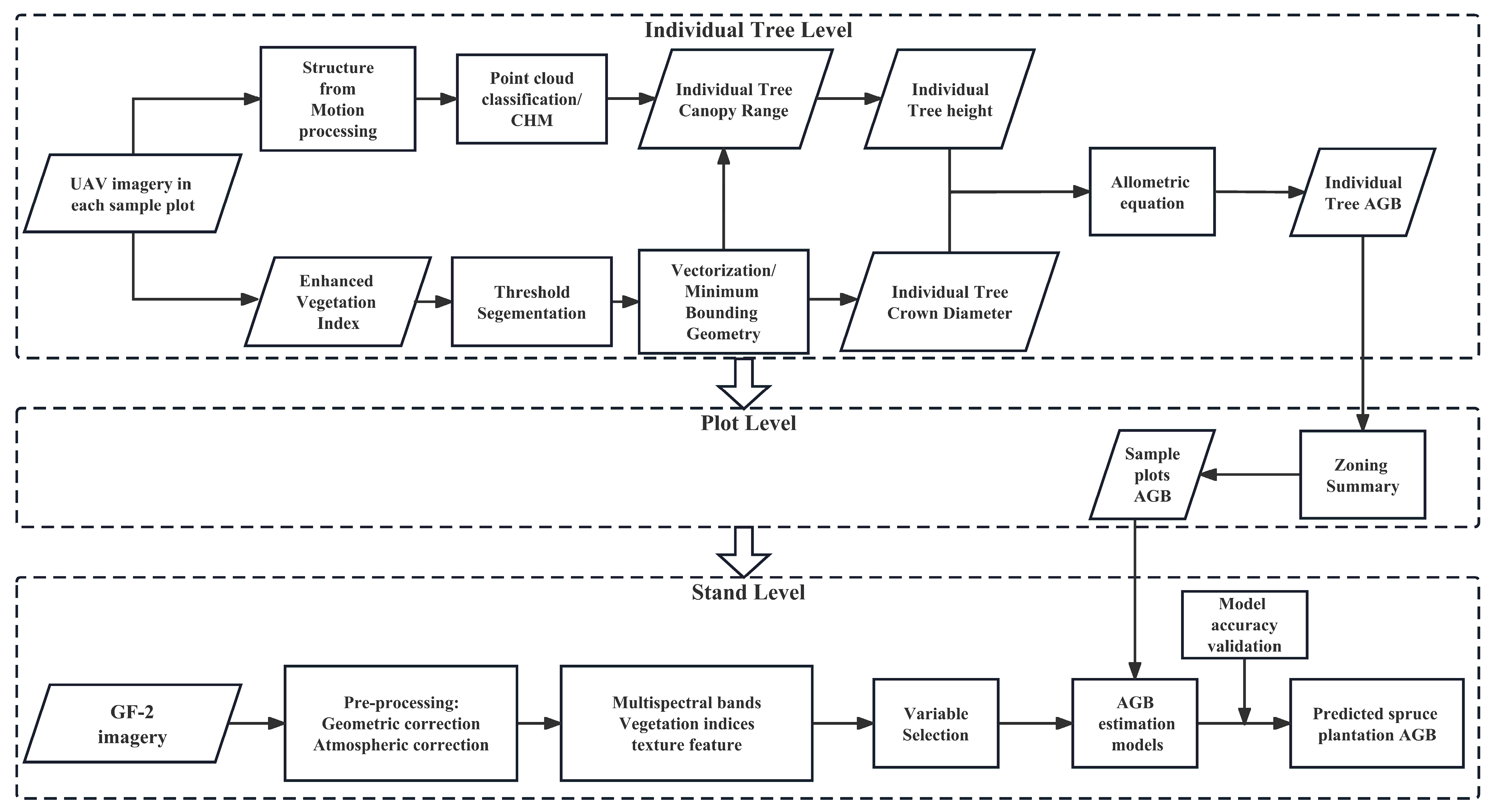
2.7. Workflow of Methodology

In this study, we aim to propose a reliable and efficient method for the large-scale estimation of the AGB in young spruce plantations by integrating UAV and GF-2 data. The proposed method consists of three main components. First, UAV data are used to acquire individual-tree structural parameters, which are then combined with an allometric equation to obtain the AGB at the individual-tree level. Second, the individual-tree-level AGB is aggregated according to designed plot divisions to achieve the plot-level AGB. Lastly, the plot-level AGB and GF-2 data are used as input variables to establish AGB estimation models. The model with the highest accuracy is then employed to predict and map the spatial distribution of the AGB in young spruce plantations. The workflow is provided in Figure 2.

3. Results

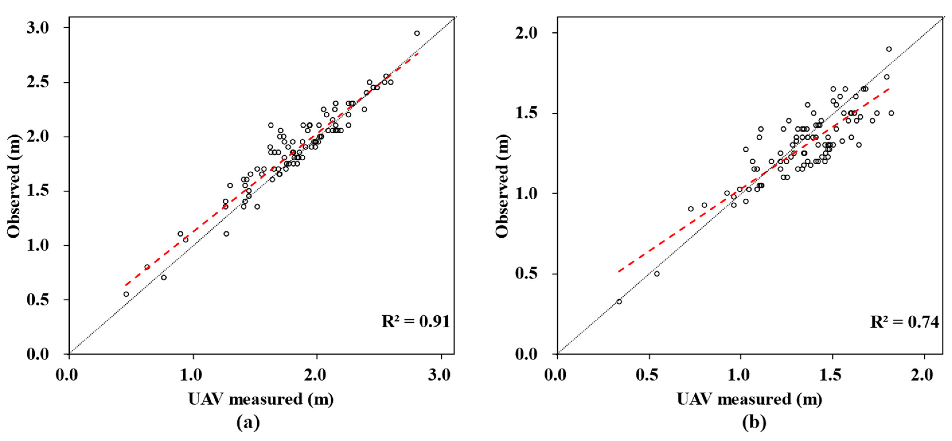
3.1. Tree Measurements

The results of the individual tree crown delineation from the UAV-derived EVI and tree height extraction from the CHM produced from the photogrammetric point cloud are shown in Figure 3.

There was a strong correlation of 0.95 between the tree heights measured in the field and those derived from the UAV images (intercept of 0 cm and slope of 1.02) (Figure 4a). A statistically significant difference was not found using a paired t-test. The 95% confidence interval for the difference between the tree height measured in the field and that derived from UAV images was from 0.02 to 0.07 m; the average difference between the tree height measured in the field and that derived from UAV images was 0.05 m. The results indicate that the UAV point cloud measurements tended to underestimate the tree heights (

Table 3. A synopsis of the tree variables that were measured and estimated (m).

	Field-Measured Tree Height	UAV-Image-Derived Tree Height	Field-Measured Tree Crown Diameter	UAV-Image-Derived Tree Crown Diameter
Minimum	0.55	0.46	0.33	0.34
Mean	1.89	1.84	1.29	1.34
Maximum	2.95	2.81	1.90	1.82

). The RMSE for individual tree heights was 0.13 m.

The tree crown diameters measured in the field and those estimated from point clouds have a strong linear relationship, as shown in Figure 4b (R² = 0.74). The crown diameters of the trees were also somewhat underestimated (95% confidence interval = from 0.02 m to 0.08 m), with a bias of 0.05 m. Between the means of the crown diameters measured in the field and those obtained from the EVI, the two-sided t-test found significant differences (p ≤ 0.05). The measurements of the tree crown had an RMSE of 0.14 m.

3.2. AGB Estimation for the Designed Sample Plots

The point clouds derived from the UAV-acquired images provided information on the crown diameters and heights of individual trees. The AGB of individual trees was calculated using the allometric equation, and then the AGB of each sample plot was obtained by partitioning and aggregating the AGB of individual trees according to the designed sample plots. The AGB at the plot level is shown in

Table 4. Summary statistics of AGB for 53 plots derived from UAV-acquired imagery (t/ha).

Number of Plots	Minimum	Mean	Maximum	Standard Deviation
53	3.41	8.63	22.13	0.61

.

3.3. Variable Importance for AGB Estimation

The VSURF algorithm quantified the importance of the variables to evaluate their ability to predict the AGB (Figure 5). It was found that multispectral bands 1, 2, and 3 were the three most important variables, followed by the VIs (NDVI, TSAVI, etc.) and the texture features derived from the GF-2 optical images. Based on the importance ranking, different combinations of variables were tried for modeling, and the best five variables, namely, B1, B2, B3, NDVI, and TSAVI, were selected for the final model.

3.4. Results and Accuracy Assessment of the AGB Model

Five variables derived from GF-2 images were used as input variables, and the AGB values, which were estimated based on UAV data, were used as output variables in the OLS, ANN, SVM, and RF models. Subsequently, we employed the Bayesian optimization algorithm to search for the optimal parameters for each machine learning model. The optimal parameters for each model were determined as follows: for the ANN, the optimal parameters were ‘batch_size’ = 4; ‘learning_rate’ = 170; ‘hidden_layer_sizes’ = 0.01; and ‘n_hidden_layers’ = 2. For the SVM, the optimal parameters were ‘C’ = 4.34; ‘gamma’ = 1.17; and ‘kernel’ = ‘linear’. For the RF, the optimal parameters were ‘n_estimators’ = 3898 and ‘max_features’ = 2. These optimal parameters were then incorporated into their respective models for further modeling. This rigorous approach to parameter optimization ensures the robustness and accuracy of our machine learning models, enhancing the reliability of our findings. Five-fold cross-validation was used to calculate the R², RMSE, MPSE, and LCCC between the observed and predicted AGB values. As shown in

Table 5. The accuracy of spruce AGB estimation by different models.

Models	R2	RMSE (t/ha)	MPSE%	LCCC
OLS	0.68	2.49	22.94	0.81
ANN	0.67	2.54	21.48	0.80
SVM	0.60	2.84	31.73	0.76
RF	0.86	1.75	15.75	0.91

, the SVM model had the lowest prediction accuracy (R² = 0.60; RMSE = 2.84 t/ha; MPSE = 31.73%; LCCC = 0.76), followed by the OLS (R² = 0.68; RMSE = 2.49 t/ha; MPSE = 22.94%; LCCC = 0.81) and ANN (R² = 0.67; RMSE = 2.54 t/ha; MPSE = 21.48%; LCCC = 0.80) models, with similar prediction accuracies. The RF model had the highest prediction accuracy (R² = 0.86; RMSE = 1.75 t/ha; MPSE = 15.75%; LCCC = 0.91), with its RMSE being 0.74, 0.79, and 1.09 lower than those of the other three models, respectively. Additionally, it had the lowest MPSE and the highest LCCC (>0.90), indicating that the predicted AGB values of the RF model were in excellent agreement with the field AGB values. The predicted AGB values from the four models did not exhibit any significant differences (p > 0.05).

Figure 6 shows the scatterplots of the AGB values for the sample plots based on the UAV data versus the model-predicted values derived from the OLS, ANN, SVM, and RF models using five-fold cross-validation. All four models’ predicted AGB values for larger values were lower than the 1:1 line, suggesting that the AGB values for the spruce plantation were underestimated, while the predictions for smaller values were greater than the line. The RF model had the highest R² and LCCC (>0.90 means excellent agreement), followed by the OLS, ANN, and SVM models, indicating that the RF model provided the best goodness of fit.

3.5. Mapping AGB of the Spruce Plantation

The AGB’s spatial distribution in the study area was mapped using the RF model, as it yielded the most accurate results (Figure 7). With a value range of from 4.44 to 17.45 t/ha and an average of 10.23 t/ha, the AGB map showed substantial geographic heterogeneity. The AGB values of the spruce plantation were higher in the northeast, west, and south of the study area than in other areas. The spatial distribution of the AGB was consistent with the temporal sequence of afforestation in spruce plantations. However, trees with lower biomass are not necessarily younger but may have poorer growing conditions. Using field surveys, Google Earth, and documentation of forest plantation plans for verification, we found that the AGB maps matched the distribution and growth of trees in the spruce plantation.

4. Discussion

4.1. Tree Measurement Method

UAV imagery has become more popular in recent years for assessing the AGB by locating trees, measuring tree heights and crown diameters, and mapping tree distributions [60,61,62,63]. In this study, we used an affordable UAV to generate a CHM and measure the AGBs of trees in sample plots. However, we used the VIs instead of the CHM to determine the tree’s location. The reason for this is the canopy structure of young spruce trees: the lowest branches are very close to the ground (Figure 3c), making it difficult to use a CHM derived from point cloud data to distinguish the canopy and ground accurately. Therefore, we used a VI to determine the canopy extent of individual trees, and then used the CHM to measure the tree height. This approach is more appropriate for young spruce plantations.

4.2. Variable Contribution for Measuring AGB in Spruce Plantations

B, G, R, NDVI, and TSAVI were selected as input parameters to estimate the AGB based on the variable-importance ranking. The NDVI is often used for estimating AGB because it represents the vegetation growth status or greenness. The TSAVI minimizes the effect of soil brightness and may be well suited for estimating the AGB in young spruce plantations with a substantial amount of bare soil. However, the visible bands (B, G, and R), which were the top three ranking parameters, are typically used to assess vegetation health and classify vegetation types; therefore, the validity of the three parameters for estimating the AGB in young spruce plantations deserves further investigation. Meanwhile, as texture features have performed well in estimating the AGB in mature forests [64,65,66], this study also included texture features for AGB estimation in young spruce forests. However, the accuracy of the model decreased after only adding the texture feature that had a high importance ranking. The reason for these results may be that the planted young forests have uniform spacing between the rows and little heterogeneous texture; thus, the results are not significant. This finding suggests that texture features may not be suitable for estimating the AGB in young spruce plantations.

4.3. Comparison of Model Suitability

The goal of this research was to uncover a model for estimating the biomass in young spruce plantations that is both precise and reliable. For its high level of convenience and accuracy in predictions, the RF model was used to build nonlinear relationships between the AGB of plots and the input variables [67]. The OLS, ANN, and SVM were chosen for AGB estimation, and the results showed that the RF model generated more precise predictions of the AGB of young spruce plantations than the OLS, ANN, and SVM models in this study area. In previous studies, ANNs have demonstrated their ability to provide reliable determinations for biomass estimation [25]. However, due to the characteristic requirement of large datasets for optimal performance, ANNs may not yield satisfactory biomass estimation results when applied to situations with limited sample sizes, as encountered in the present study. This constraint highlights the importance of considering alternative methods or adapting ANN-based approaches to accommodate smaller datasets in order to achieve more accurate and reliable biomass estimations.

The optimum split for each node of the standard regression tree is used to randomly choose a subset of all variables in bootstrap sampling and variable sampling, which is a significant benefit of RFs [68]. The RF model’s generalization ability and resistance to anticipated data are both enhanced by its relative insensitivity to changes in the inputs; as a result, the RF model is better equipped to cope with the difficulties of overfitting and multicollinearity [69]. Our results indicate that the RF model is a valuable exploratory and predictive method for estimating the AGB of young spruce plantations.

4.4. Limitations and Sources of Errors

The tree structure parameters derived from UAV images were tested on a validation sample of 97 trees, but plot-level AGB estimations were not. Future research will focus on measuring the uncertainty of the UAV-image-based AGB estimate at the plot level.

All four models have different degrees of underestimation at high values when estimating AGB, which may be due to the following two reasons: Reason 1 could be that the field AGBs are mostly lower values and less in number at the high values, which would cause the models to fail to make robust predictions for these data, and the predicted values would tend to be in the intervals with more field AGBs. Reason 2 may be that the pixels of each optical image contain more soil information due to the small tree canopy, thereby making the optical images not truly reflect the vegetation information in the areas with higher values of field AGB.

The spatial resolution of the GF-2 MSI data is 3.2 m. If a sample plot size of 30 × 30 m is used in this study (a commonly used plot size in forestry), then the scale effect may adversely impact the AGB estimation results. As this study focused on the semiautomated processing of UAV data to obtain the AGB of the sample plots, the sample plot size can be closer to the spatial resolution of the GF-2 data to minimize the adverse results of the scale effect. A future study will focus on how much the adverse impact of the scale effect can be mitigated by choosing an appropriate plot size.

This method for estimating AGB was specifically designed to address the neat and sparse forest spatial distribution characteristics of the young spruce plantations in this region, and the results are repeatable for young plantations of spruce or other tree species in this region. However, it may not be as effective in other densely forested areas.

In addition, due to various reasons, such as cloud contamination, the image date did not match the sampling date. We selected an image closest to the sampling date. This discrepancy may have caused a slight error in the AGB estimation results, although the AGB variation caused by the different dates may not be significant.

5. Conclusions

Integrating UAV and satellite optical data supported the development of a new method to estimate the AGB of young spruce forests on a broad scale, which is the primary contribution of this study. This approach is superior to traditional field plot measurements because it allows for the semiautomatic extraction of the structural parameters of trees from low-cost UAV-derived photogrammetric point clouds. The accuracy evaluation revealed that the structural parameters of individual trees were accurately estimated, indicating that the proposed workflow could be used to collect precise measurements of sampling plots rapidly from remote areas.

The results from this research also support the effectiveness of the RF model in predicting the AGB in spruce plantations. The RF model has better estimation accuracy than the other three models, as its RMSE and MPSE are lower than those of the other three models, and its R² and LCCC (>0.90 means excellent agreement) values were higher. The resulting AGB map was in good agreement with field surveys, documentation of forest plantation plans, and the temporal sequence of the afforestation of the spruce plantations. The results proved that the RF model with multiple data sources (UAV and GF-2 optical images) could produce reliable AGB models and geographical distribution maps of young spruce plantations. The UAV data could effectively provide structural parameters of young spruce plantation trees, such as tree heights and crown diameters, for AGB modeling. Future targeted research is needed to improve the accuracy of extracting individual-tree structural parameters from young spruce plantations to support the AGB monitoring of spruce under different plantation and landscape conditions.

References

1. Rockström, J.; Beringer, T.; Hole, D.; Griscom, B.; Mascia, M.B.; Folke, C.; Creutzig, F. We need biosphere stewardship that protects carbon sinks and builds resilience. Proc. Natl. Acad. Sci. USA 2021, 118, e2115218118. [Google Scholar] [CrossRef] [PubMed]
2. Yang, Y.; Shi, Y.; Sun, W.; Chang, J.; Zhu, J.; Chen, L.; Wang, X.; Guo, Y.; Zhang, H.; Yu, L.; et al. Terrestrial carbon sinks in China and around the world and their contribution to carbon neutrality. Sci. China Life Sci. 2022, 65, 861–895. [Google Scholar] [CrossRef] [PubMed]
3. Li, M. Carbon Storages and Carbon Sequestration Potentials of the Terrestrial Ecosystems on the Loess Plateau; Chinese Academy of Sciences and Ministry of Education (Research Center of Research Center Soil and Water Conservation and Ecological Environment): Beijing, China, 2021. [Google Scholar]
4. Fan, B.; Li, X.; Du, J. Review and Prospect of Forestry Policies of the CPC in the Past Century. For. Econ. 2021, 43, 5–23. [Google Scholar] [CrossRef]
5. Yong, L.; Lan, G. Implementation Path and Mode Selection of China’s Carbon Neutralization Goal. J. South China Agric. Univ. (Soc. Sci. Ed.) 2021, 20, 77–93. [Google Scholar]
6. Liu, R.; Wang, D.; Li, P.; Jin, Y.; Liang, S. Plant diversity, ground biomass characteristics and their relationships of typical plantations in the alpine region of Qinghai. Acta Ecol. Sin. 2020, 40, 692–700. [Google Scholar]
7. Guo, Z.; Cao, C.; Liu, P. Construction of biomass model of Chinese fir plantation in Guangdong based on Lianqing data. J. Cent. South Univ. For. Technol. 2022, 42, 78–89. [Google Scholar] [CrossRef]
8. Zhang, L.; Yu, P.; Wang, Y.; Wang, S.; Liu, X. Biomass change of middle aged forest of Qinghai spruce along an altitudinal gradient on the north slope of Qilian Mountains. Sci. Silva. Sin 2015, 51, 4–10. [Google Scholar]
9. Xu, Z.; Zhao, C.; Feng, Z.; Zhang, F.; Sher, H.; Wang, C.; Peng, H.; Wang, Y.; Zhao, Y.; Wang, Y. Estimating realized and potential carbon storage benefits from reforestation and afforestation under climate change: A case study of the Qinghai spruce forests in the Qilian Mountains, northwestern China. Mitig. Adapt. Strateg. Glob. Chang. 2013, 18, 1257–1268. [Google Scholar] [CrossRef]
10. Shou-zhang, P.; Chuan-yan, Z.; Xiang-lin, Z.; Zhong-lin, X.; Lei, H. Spatial distribution characteristics of the biomass and carbon storage of Qinghai spruce (Picea crassifolia) forests in Qilian Mountains. Yingyong Shengtai Xuebao 2011, 22, 1689–1694. [Google Scholar]
11. Köhl, M.; Magnussen, S.; Marchetti, M. Sampling Methods, Remote Sensing and GIS Multiresource Forest Inventory; Springer: Berlin/Heidelberg, Germany, 2006; Volume 2. [Google Scholar]
12. Gardner, T.A.; Barlow, J.; Araujo, I.S.; Ávila-Pires, T.C.; Bonaldo, A.B.; Costa, J.E.; Esposito, M.C.; Ferreira, L.V.; Hawes, J.; Hernandez, M.I.M.; et al. The cost-effectiveness of biodiversity surveys in tropical forests. Ecol. Lett. 2008, 11, 139–150. [Google Scholar] [CrossRef]
13. Mao, C.; Yi, L.; Xu, W.; Dai, L.; Bao, A.; Wang, Z.; Zheng, X. Study on Biomass Models of Artificial Young Forest in the Northwestern Alpine Region of China. Forests 2022, 13, 1828. [Google Scholar] [CrossRef]
14. Kumar, L.; Mutanga, O. Remote Sensing of Above-Ground Biomass. Remote Sens. 2017, 9, 935. [Google Scholar] [CrossRef] [Green Version]
15. Meng, B.P.; Liang, T.G.; Yi, S.H.; Yin, J.P.; Cui, X.; Ge, J.; Hou, M.J.; Lv, Y.Y.; Sun, Y. Modeling Alpine Grassland Above Ground Biomass Based on Remote Sensing Data and Machine Learning Algorithm: A Case Study in East of the Tibetan Plateau, China. IEEE J. Sel. Top. Appl. Earth Obs. Remote Sens. 2020, 13, 2986–2995. [Google Scholar] [CrossRef]
16. Baccini, A.; Laporte, N.; Goetz, S.J.; Sun, M.; Dong, H. A first map of tropical Africa’s above-ground biomass derived from satellite imagery. Environ. Res. Lett. 2008, 3, 045011. [Google Scholar] [CrossRef] [Green Version]
17. Zhu, X.; Liu, D. Improving forest aboveground biomass estimation using seasonal Landsat NDVI time-series. Isprs J. Photogramm. Remote Sens. 2015, 102, 222–231. [Google Scholar] [CrossRef]
18. Gou, R.-K.; Chen, J.-Q.; Duan, G.-H.; Yang, R.; Bu, Y.-K.; Zhao, J.; Zhao, P.-X. Inversion of aboveground biomass of Pinus tabuliformis plantations based on GF-2 data. Yingyong Shengtai Xuebao 2019, 30, 4031–4040. [Google Scholar] [CrossRef]
19. Hadush, T.; Girma, A.; Zenebe, A. Tree Height Estimation from Unmanned Aerial Vehicle Imagery and Its Sensitivity on Above Ground Biomass Estimation in Dry Afromontane Forest, Northern Ethiopia. Momona Ethiop. J. Sci. 2021, 13, 256–280. [Google Scholar] [CrossRef]
20. Jones, A.R.; Segaran, R.R.; Clarke, K.D.; Waycott, M.; Goh, W.S.H.; Gillanders, B.M. Estimating Mangrove Tree Biomass and Carbon Content: A Comparison of Forest Inventory Techniques and Drone Imagery. Front. Mar. Sci. 2020, 6, 784. [Google Scholar] [CrossRef] [Green Version]
21. Li, X.; Zhang, M.; Long, J.; Lin, H. A novel method for estimating spatial distribution of forest above-ground biomass based on multispectral fusion data and ensemble learning algorithm. Remote Sens. 2021, 13, 3910. [Google Scholar] [CrossRef]
22. Zhu, Y.; Liu, K.W.; Myint, S.; Du, Z.; Li, Y.; Cao, J.; Liu, L.; Wu, Z. Integration of GF2 Optical, GF3 SAR, and UAV Data for Estimating Aboveground Biomass of China’s Largest Artificially Planted Mangroves. Remote Sens. 2020, 12, 2039. [Google Scholar] [CrossRef]
23. Chen, H.; Qin, Z.; Zhai, D.-L.; Ou, G.; Li, X.; Zhao, G.; Fan, J.; Zhao, C.; Xu, H. Mapping Forest Aboveground Biomass with MODIS and Fengyun-3C VIRR Imageries in Yunnan Province, Southwest China Using Linear Regression, K-Nearest Neighbor and Random Forest. Remote Sens. 2022, 14, 5456. [Google Scholar] [CrossRef]
24. Ji, Y.; Xu, K.; Zeng, P.; Zhang, W. GA-SVR Algorithm for Improving Forest Above Ground Biomass Estimation Using SAR Data. IEEE J. Sel. Top. Appl. Earth Obs. Remote Sens. 2021, 14, 6585–6595. [Google Scholar] [CrossRef]
25. Vahedi, A.A. Artificial neural network application in comparison with modeling allometric equations for predicting above-ground biomass in the Hyrcanian mixed-beech forests of Iran. Biomass Bioenergy 2016, 88, 66–76. [Google Scholar] [CrossRef]
26. Nguyen, T.H.; Jones, S.; Soto-Berelov, M.; Haywood, A.; Hislop, S. A Comparison of Imputation Approaches for Estimating Forest Biomass Using Landsat Time-Series and Inventory Data. Remote Sens. 2018, 10, 1825. [Google Scholar] [CrossRef] [Green Version]
27. Gleason, C.J.; Im, J. Forest biomass estimation from airborne LiDAR data using machine learning approaches. Remote Sens. Environ. 2012, 125, 80–91. [Google Scholar] [CrossRef]
28. Remondino, F.; Spera, M.G.; Nocerino, E.; Menna, F.; Nex, F. State of the art in high density image matching. Photogramm. Rec. 2014, 29, 144–166. [Google Scholar] [CrossRef] [Green Version]
29. Gehrke, S.; Morin, K.; Downey, M.; Boehrer, N.; Fuchs, T. Semi-global matching: An alternative to LIDAR for DSM generation. In Proceedings of the 2010 Canadian Geomatics Conference and Symposium of Commission I, Calgary, AB, Canada, 15–18 June 2010. [Google Scholar]
30. Vastaranta, M.; Wulder, M.A.; White, J.C.; Pekkarinen, A.; Tuominen, S.; Ginzler, C.; Kankare, V.; Holopainen, M.; Hyyppä, J.; Hyyppä, H. Airborne laser scanning and digital stereo imagery measures of forest structure: Comparative results and implications to forest mapping and inventory update. Can. J. Remote Sens. 2013, 39, 382–395. [Google Scholar] [CrossRef]
31. Gülci, S. The determination of some stand parameters using SfM-based spatial 3D point cloud in forestry studies: An analysis of data production in pure coniferous young forest stands. Environ. Monit. Assess. 2019, 191, 495. [Google Scholar] [CrossRef]
32. Minařík, R.; Langhammer, J.; Lendzioch, T. Automatic Tree Crown Extraction from UAS Multispectral Imagery for the Detection of Bark Beetle Disturbance in Mixed Forests. Remote Sens. 2020, 12, 4081. [Google Scholar] [CrossRef]
33. Koch, B.; Heyder, U.; Weinacker, H. Detection of individual tree crowns in airborne lidar data. Photogramm. Eng. Remote Sens. 2006, 72, 357–363. [Google Scholar] [CrossRef] [Green Version]
34. Ke, Y.; Quackenbush, L.J. A review of methods for automatic individual tree-crown detection and delineation from passive remote sensing. Int. J. Remote Sens. 2011, 32, 4725–4747. [Google Scholar] [CrossRef]
35. Senf, C.; Seidl, R.; Hostert, P. Remote sensing of forest insect disturbances: Current state and future directions. Int. J. Appl. Earth Obs. Geoinf. 2017, 60, 49–60. [Google Scholar] [CrossRef] [Green Version]
36. Klouček, T.; Komárek, J.; Surový, P.; Hrach, K.; Janata, P.; Vašíček, B. The use of UAV mounted sensors for precise detection of bark beetle infestation. Remote Sens. 2019, 11, 1561. [Google Scholar] [CrossRef] [Green Version]
37. Näsi, R.; Honkavaara, E.; Lyytikäinen-Saarenmaa, P.; Blomqvist, M.; Litkey, P.; Hakala, T.; Viljanen, N.; Kantola, T.; Tanhuanpää, T.; Holopainen, M. Using UAV-based photogrammetry and hyperspectral imaging for mapping bark beetle damage at tree-level. Remote Sens. 2015, 7, 15467–15493. [Google Scholar] [CrossRef] [Green Version]
38. Mweresa, I.A.; Odera, P.A.; Kuria, D.N.; Kenduiywo, B.K. Estimation of tree distribution and canopy heights in ifakara, tanzania using unmanned aerial system (UAS) stereo imagery. Am. J. Geogr. Inf. Syst. 2017, 6, 187–200. [Google Scholar]
39. Goodbody, T.R.H.; Coops, N.C.; Hermosilla, T.; Tompalski, P.; Crawford, P. Assessing the status of forest regeneration using digital aerial photogrammetry and unmanned aerial systems. Int. J. Remote Sens. 2018, 39, 5246–5264. [Google Scholar] [CrossRef]
40. Bai, Y.J. Project Description: Afforestation Project in Xining City. Available online: https://registry.verra.org/app/projectDetail/VCS/1825 (accessed on 25 May 2022).
41. Wang, D.; Zhou, X.; He, K.; Li, S.; Shi, C.; Chang, G. The potential productivity of the main species used in the Datong reafforestation project on former farmland, Qinghai Province. Acta Ecol. Sin. 2004, 24, 2984–2990. [Google Scholar]
42. Minghui, S. Object-oriented Urban Land Classfication with GF-2 Remote Sensing Image. Remote Sens. Technol. Appl. 2019, 34, 547–552+629. [Google Scholar]
43. Otsu, N. A threshold selection method from gray-level histograms. IEEE Trans. Syst. Man Cybern. 1979, 9, 62–66. [Google Scholar] [CrossRef] [Green Version]
44. Zheng, X.T.; Yi, L.B.; Li, Q.F.; Bao, A.M.; Wang, Z.Y.; Xu, W.Q. Developing biomass estimation models of young trees in typical plantation on the Qinghai-Tibet Plateau, China. Chin. J. Appl. Ecol. 2022, 33, 2923–2935. [Google Scholar] [CrossRef]
45. Pham, L.T.H.; Brabyn, L. Monitoring mangrove biomass change in Vietnam using SPOT images and an object-based approach combined with machine learning algorithms. ISPRS J. Photogramm. Remote Sens. 2017, 128, 86–97. [Google Scholar] [CrossRef]
46. Breiman, L. Random Forests. Mach. Learn. 2001, 45, 5–32. [Google Scholar] [CrossRef] [Green Version]
47. Gregorutti, B.; Michel, B.; Saint-Pierre, P. Correlation and variable importance in random forests. Stat. Comput. 2017, 27, 659–678. [Google Scholar] [CrossRef] [Green Version]
48. Genuer, R.; Poggi, J.-M.; Tuleau-Malot, C. VSURF: An R package for variable selection using random forests. R J. 2015, 7, 19–33. [Google Scholar] [CrossRef] [Green Version]
49. Tang, Y.; Ali, A.; Feng, L.H. Bayesian model predicts the aboveground biomass of Caragana microphylla in sandy lands better than OLS regression models. J. Plant Ecol. 2020, 13, 732–737. [Google Scholar] [CrossRef]
50. Yang, S.; Feng, Q.; Liang, T.; Liu, B.; Zhang, W.; Xie, H. Modeling grassland above-ground biomass based on artificial neural network and remote sensing in the Three-River Headwaters Region. Remote Sens. Environ. 2018, 204, 448–455. [Google Scholar] [CrossRef]
51. Qiu, S.; Xing, Y.; Tian, J.; Ding, J. Forest Canopy Height Estimation of Large Area Using Spaceborne LIDAR and HJ-1A/HSI Hyperspectral Imageries. Sci. Silvae Sin. 2016, 52, 142–149. [Google Scholar]
52. Pal, M. Random forest classifier for remote sensing classification. Int. J. Remote Sens. 2005, 26, 217–222. [Google Scholar] [CrossRef]
53. Nelson, R.; Ranson, K.; Sun, G.; Kimes, D.; Kharuk, V.; Montesano, P. Estimating Siberian timber volume using MODIS and ICESat/GLAS. Remote Sens. Environ. 2009, 113, 691–701. [Google Scholar] [CrossRef]
54. Englhart, S.; Keuck, V.; Siegert, F. Modeling aboveground biomass in tropical forests using multi-frequency SAR data—A comparison of methods. IEEE J. Sel. Top. Appl. Earth Obs. Remote Sens. 2011, 5, 298–306. [Google Scholar] [CrossRef]
55. Carreiras, J.M.; Vasconcelos, M.J.; Lucas, R.M. Understanding the relationship between aboveground biomass and ALOS PALSAR data in the forests of Guinea-Bissau (West Africa). Remote Sens. Environ. 2012, 121, 426–442. [Google Scholar] [CrossRef]
56. Snoek, J.; Larochelle, H.; Adams, R.P. Practical bayesian optimization of machine learning algorithms. In Advances in Neural Information Processing Systems; Princeton University: Princeton, NJ, USA, 2012; Volume 25. [Google Scholar]
57. Zhao, D.; Arshad, M.; Wang, J.; Triantafilis, J. Soil exchangeable cations estimation using Vis-NIR spectroscopy in different depths: Effects of multiple calibration models and spiking. Comput. Electron. Agric. 2021, 182, 105990. [Google Scholar] [CrossRef]
58. Zhao, D.; Arshad, M.; Li, N.; Triantafilis, J. Predicting soil physical and chemical properties using vis-NIR in Australian cotton areas. CATENA 2021, 196, 104938. [Google Scholar] [CrossRef]
59. Zhao, D.; Wang, J.; Zhao, X.; Triantafilis, J. Clay content mapping and uncertainty estimation using weighted model averaging. CATENA 2022, 209, 105791. [Google Scholar] [CrossRef]
60. Iizuka, K.; Yonehara, T.; Itoh, M.; Kosugi, Y. Estimating Tree Height and Diameter at Breast Height (DBH) from Digital Surface Models and Orthophotos Obtained with an Unmanned Aerial System for a Japanese Cypress (Chamaecyparis obtusa) Forest. Remote Sens. 2018, 10, 13. [Google Scholar] [CrossRef] [Green Version]
61. Panagiotidis, D.; Abdollahnejad, A.; Surový, P.; Chiteculo, V. Determining tree height and crown diameter from high-resolution UAV imagery. Int. J. Remote Sens. 2017, 38, 2392–2410. [Google Scholar] [CrossRef]
62. Mohan, M.; Silva, C.A.; Klauberg, C.; Jat, P.; Catts, G.; Cardil, A.; Hudak, A.T.; Dia, M. Individual Tree Detection from Unmanned Aerial Vehicle (UAV) Derived Canopy Height Model in an Open Canopy Mixed Conifer Forest. Forests 2017, 8, 340. [Google Scholar] [CrossRef] [Green Version]
63. Otero, V.; Van De Kerchove, R.; Satyanarayana, B.; Martínez-Espinosa, C.; Fisol, M.A.B.; Ibrahim, M.R.B.; Sulong, I.; Mohd-Lokman, H.; Lucas, R.; Dahdouh-Guebas, F. Managing mangrove forests from the sky: Forest inventory using field data and Unmanned Aerial Vehicle (UAV) imagery in the Matang Mangrove Forest Reserve, peninsular Malaysia. For. Ecol. Manag. 2018, 411, 35–45. [Google Scholar] [CrossRef]
64. Migolet, P.; Goita, K.; Pambo, A.F.K.; Mambimba, A.N. Estimation of the total dry aboveground biomass in the tropical forests of Congo Basin using optical, LiDAR, and radar data. Giscience Remote Sens. 2022, 59, 431–460. [Google Scholar] [CrossRef]
65. Liang, Y.Y.; Kou, W.L.; Lai, H.Y.; Wang, J.; Wang, Q.H.; Xu, W.H.; Wang, H.; Lu, N. Improved estimation of aboveground biomass in rubber plantations by fusing spectral and textural information from UAV-based RGB imagery. Ecol. Indic. 2022, 142, 109286. [Google Scholar] [CrossRef]
66. Ehlers, D.; Wang, C.; Coulston, J.; Zhang, Y.L.; Pavelsky, T.; Frankenberg, E.; Woodcock, C.; Song, C.H. Mapping Forest Aboveground Biomass Using Multisource Remotely Sensed Data. Remote Sens. 2022, 14, 1115. [Google Scholar] [CrossRef]
67. Wang, D.; Wan, B.; Liu, J.; Su, Y.; Guo, Q.; Qiu, P.; Wu, X. Estimating aboveground biomass of the mangrove forests on northeast Hainan Island in China using an upscaling method from field plots, UAV-LiDAR data and Sentinel-2 imagery. Int. J. Appl. Earth Obs. Geoinf. 2020, 85, 101986. [Google Scholar] [CrossRef]
68. Cutler, D.R.; Edwards, T.C., Jr.; Beard, K.H.; Cutler, A.; Hess, K.T.; Gibson, J.; Lawler, J.J. Random Forests for classification in Ecology. Ecology 2007, 88, 2783–2792. [Google Scholar] [CrossRef] [PubMed]
69. Fukuda, S.; Yasunaga, E.; Nagle, M.; Yuge, K.; Sardsud, V.; Spreer, W.; Müller, J. Modelling the relationship between peel colour and the quality of fresh mango fruit using Random Forests. J. Food Eng. 2014, 131, 7–17. [Google Scholar] [CrossRef]
Figure 1. Study area. (a) Location of the surrounding areas of the study area (red rectangle) in China. (b) Location of the study area (yellow pentacle) in Qinghai Province. (c) Study area on a multispectral image and location of UAV sample plots.
Sustainability 15 09700 g001
Figure 2. The workflow for estimating 3-level AGB of spruce plantation using UAV and GF-2 multispectral imagery.
Sustainability 15 09700 g002
Figure 3. (a) Example of individual tree crown delineation from UAV-image-derived EVI using threshold segmentation and the minimum boundary geometry (MBG) in a sample plot. The color combination of the base image is NIR, R, and G. (b) Location of the example sample plot in the study area. (c) Three-dimensional profile of the trees inside the red rectangle in subplot (a).
Sustainability 15 09700 g003
Figure 4. Scatterplot between (a) the tree heights measured in the field and estimated from UAV-derived point clouds and (b) the field-measured and UAV-image-derived tree crown diameters (m). The measurements of the point clouds derived from UAV images and field data are fitted linearly, as shown by the red line. The grey line indicates the 1:1 line.
Sustainability 15 09700 g004
Figure 5. Variable-importance measures generated by VSURF including all variables (TEXTURE_B1-32 are the results of calculating 8 texture features for each of the 4 bands).
Sustainability 15 09700 g005
Figure 6. Scatterplots between the AGB of sample plots based on the UAV data and predicted AGB obtained from the (a) OLS model, (b) ANN model, (c) SVM model, and (d) RF model. The AGB values based on the UAV data and the predicted AGB values of each model are fitted linearly, as shown by the red line.
Sustainability 15 09700 g006
Figure 7. Spatial distribution of the spruce plantation’s AGB.
Sustainability 15 09700 g007