Estimating Inter-Regional Freight Demand in China Based on the Input–Output Model

Abstract

The inter-regional freight volume is a crucial factor for transportation infrastructure planning and investment decision-making. However, existing studies on freight volume estimation have mainly focused on the total freight volume within a specific region, without taking freight flow into consideration. In this research, a gravity model was employed to estimate the inter-regional trade coefficient matrix based on the input–output tables of the 31 provinces in China in 2017. The inter-regional freight volume was then determined by converting the value flow into freight flow. To determine the model parameters, we used information from 2017 and subsequently validated the results using dates from 2012 to 2020. We also studied the impact of industrial structure change on freight volume by simulating dates from the aforementioned model in 2017. The results indicated that the model can effectively simulate inter-regional freight volume while taking into account the influence of industrial restructuring.

1. Introduction

Several disciplines have recently paid more attention to the role that freight transportation has in the national transportation network [1,2]. The development of the local economy and the management of relevant logistics infrastructure construction can both be supported by accurate freight volume forecasting. The expansion of important infrastructures, including roads, railroads, shipping, warehousing, and trans-shipment activities has been made possible by the increasing volume of freight, allowing for the widespread mobility and growing inter-regional populations, as well as technological advancement and specialization. The need for inter-regional economic exchanges, which reflects the level of social development and the general standard of living, drives the demand for inter-regional freight volume [3]. It is also a crucial metric for determining the level of regional economic competitiveness. In order to improve economic development and boost the inter-regional economic growth, inter-regional freight volume forecasts can be used to more effectively modify the construction of pertinent logistics infrastructure in a region. Presently, China is executing its strategy to emerge as a significant transportation nation. It is planning several extensive cross-regional transportation construction projects, including the Sichuan–Tibet Railway (Ya’an to Linzhi section), the Jing–Xin Expressway (Balikun to Mukti section), and the new western land–sea corridor (Pinglu canal). The planning and management of these construction projects necessitate the computation of inter-regional freight volumes.

Internationally, the gravity model (GM), the spatial general equilibrium model (SCGE), the multi-regional Input–Output model (IO), and regression analysis have been widely used for the quantitative forecasting of such volumes. Several scholars have predicted freight and passenger volume based on the GM theory [4,5,6,7,8,9], and other have used the GM to study network security, the development of economic and trade relations, economic development model, and trade potential [10,11,12,13]. Despite the statistical verifiability of its results, the GM’s lack of detail limits its usefulness in predicting freight volume. Scholars have used SCGE for inter-regional economic evaluation and inter-regional freight volume prediction [14,15,16,17,18], as well as for studied oil price volatility, optimal carbon tax rate, shadow economy, and other aspects based on its theory [19,20,21,22,23,24,25]. The SCGE fully considers the side effects of income and supply. The current practice is to estimate some major model parameters using econometric methods and then to calibrate the other parameters for the dataset of the base year. However, not all major behavioral equations can be estimated through econometrics. Several scholars have conducted research on inter-regional economic exchange and inter-regional freight volume forecasting based on the IO [26,27,28,29], and others have used the IO to analyze the impact of electric vehicles, energy and resource tax reform, building energy consumption, and other factors on the economy and society [30,31,32,33,34,35,36]. The IO, applied extensively in research on inter-regional economic exchange and freight volume forecasting, systematically elucidates the economic links between provinces and sectors. Nevertheless, it overlooks the impact of significant changes in transportation policy and infrastructure on the regional economies.

Regarding the economic exchanges between provinces in China, due to the absence of institutions like customs, data collection hurdles lead to a scarcity of comprehensive statistical data, making the input–output method difficult. Consequently, the simulation of China’s freight volume focuses on the total volume, with inter-regional freight volume simulation being seldom reported. For example, scholars have studied freight volume, trade flow, and economic flow based on the Pearson correlation analysis, fuzzy linear regression model, and the GM [37,38,39,40].

This study introduced a novel freight demand forecasting model based on input–output statistics for 42 sectors in the 31 Chinese provinces. This model calculated the inter-regional trade coefficient matrix and column coefficient model, taking into account the changes in regional GDP and industrial structure. Using the GM, it estimated the column coefficient model and inter-regional trade coefficient matrix, which were used to construct inter-regional input–output tables. These tables transformed inter-regional value flows into freight flows, determining inter-regional freight volumes. This model provided a quantitative methodology for analyzing the impact of industrial structure on freight volume. It provided the foundational data for determining the investment scale, construction standard, and basic transportation capacity required by related projects in each region. Furthermore, it offered freight volume data support and a basis for decisions related to operation, maintenance, personnel deployment, and plans at the project’s operation stage.

2. Data Collection and Methodology

2.1. Data Collection

(1)

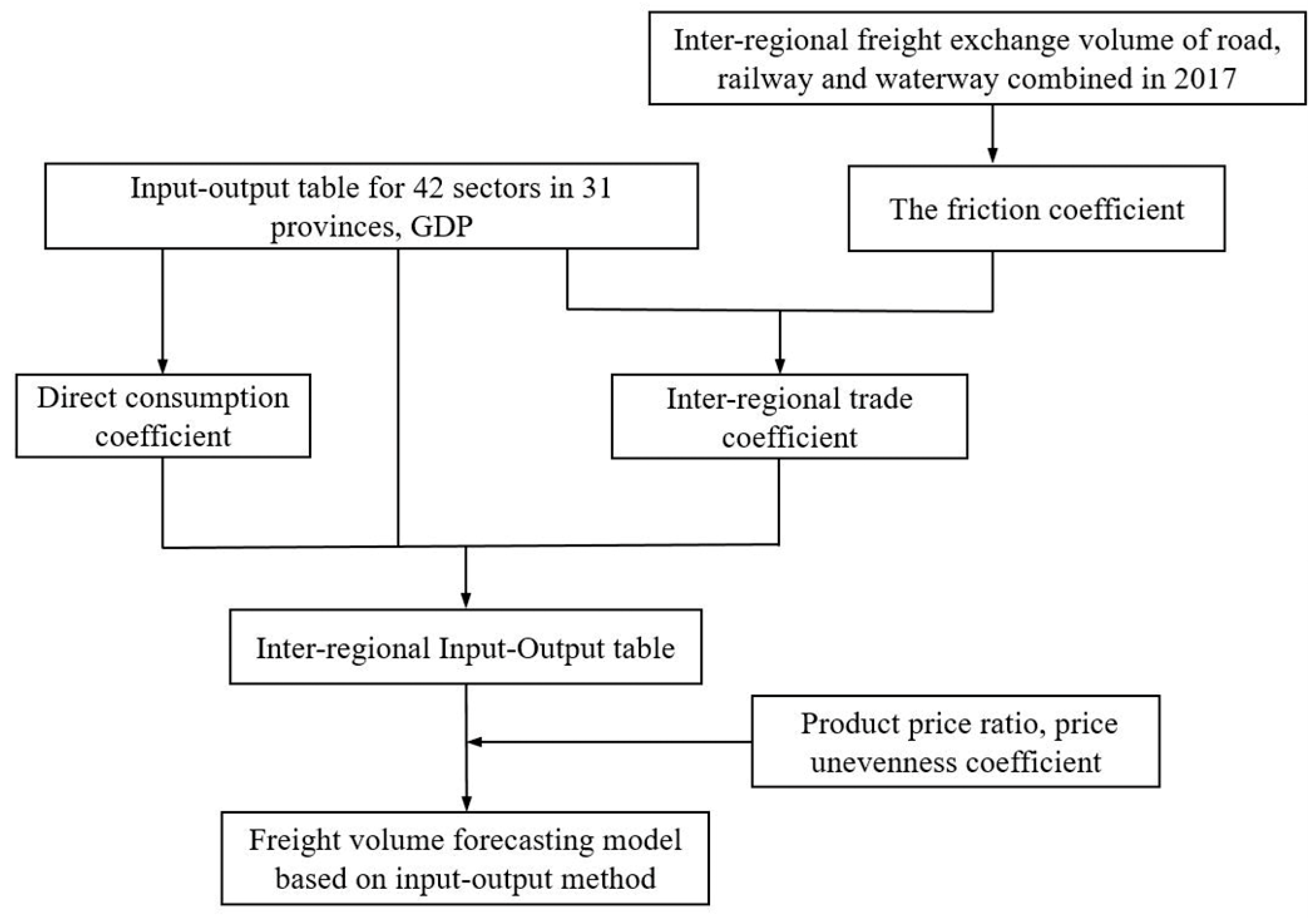
Input–Output table. The Input–Output table reflects the inter-relationship and balance between various departments in a certain period. China has systematically compiled regional input–output tables every 5 years since 1987 for its 31 provinces, with the latest version published in 2017. These tables divide sectors (S1–S42) into three industries: sector S1 represents the primary industry, sectors S2–S28 represent the secondary industry, and sectors S29–S42 represent the tertiary industry. In this study, the model parameters were calibrated using 2017′s date and validated against data from 2012 to 2020. The regional input–output tables for 31 provinces in 2017 were drawn from the China Regional Input–Output Tables 2017 [41].

(2)

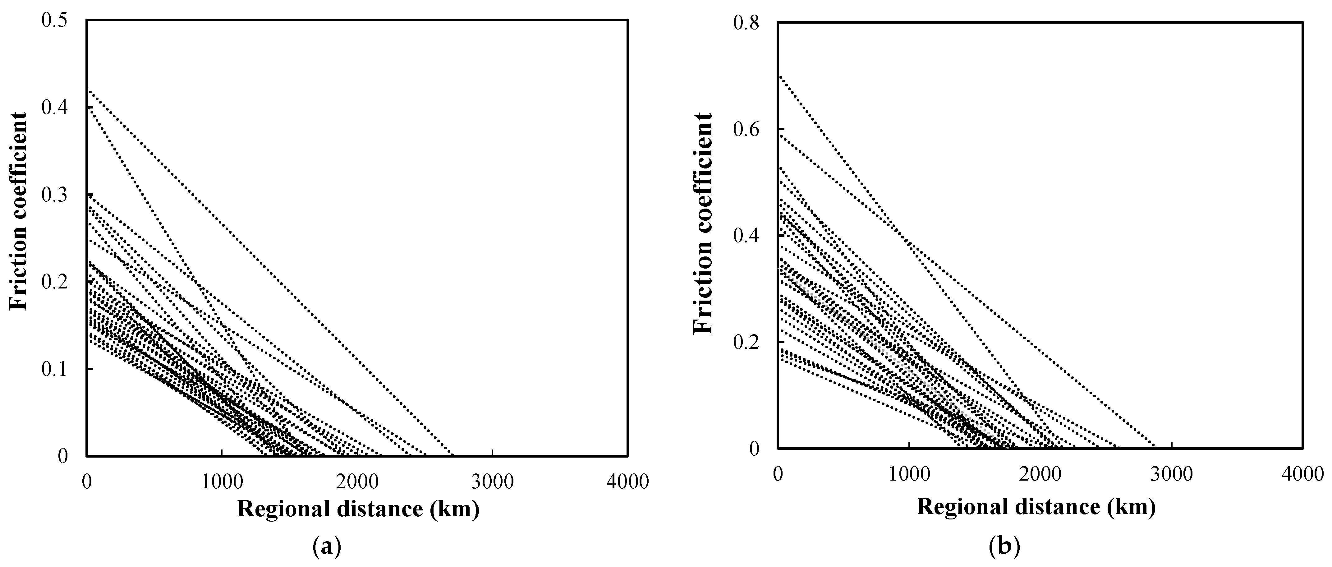
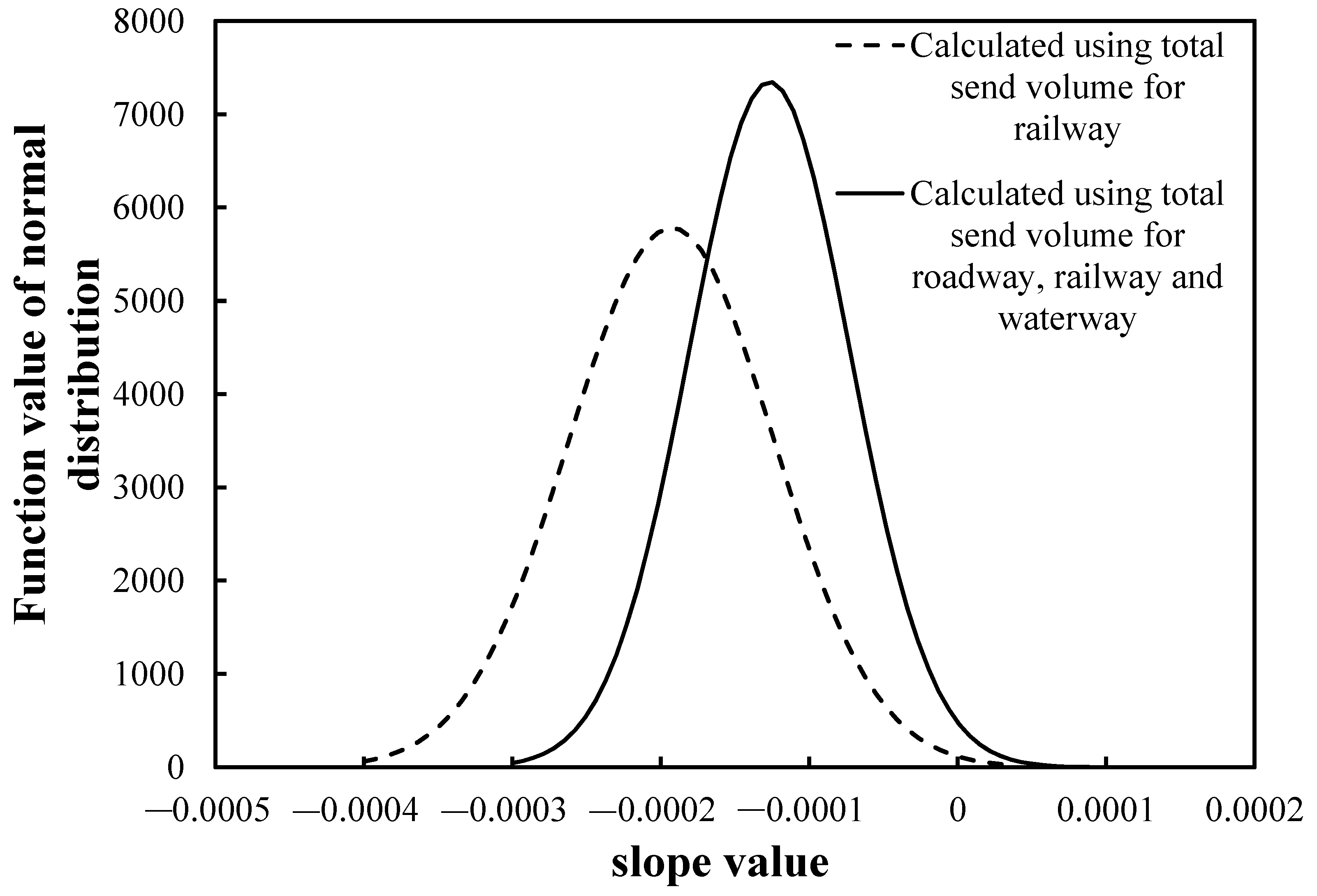
Freight volume. We considered the total freight volume and freight exchange volume of roads, waterways, and railways across China’s provinces. The total freight volume for China’s 31 provinces from 2012 to 2020, sourced from the China Statistical Yearbook, was compared with the total freight volume simulated by the model. The freight exchange volume date for roadways, waterways, and railways from 2012 to 2020 were extracted from the China Transport Yearbook. These data were then summated to calculate the friction coefficient [42].

(3)

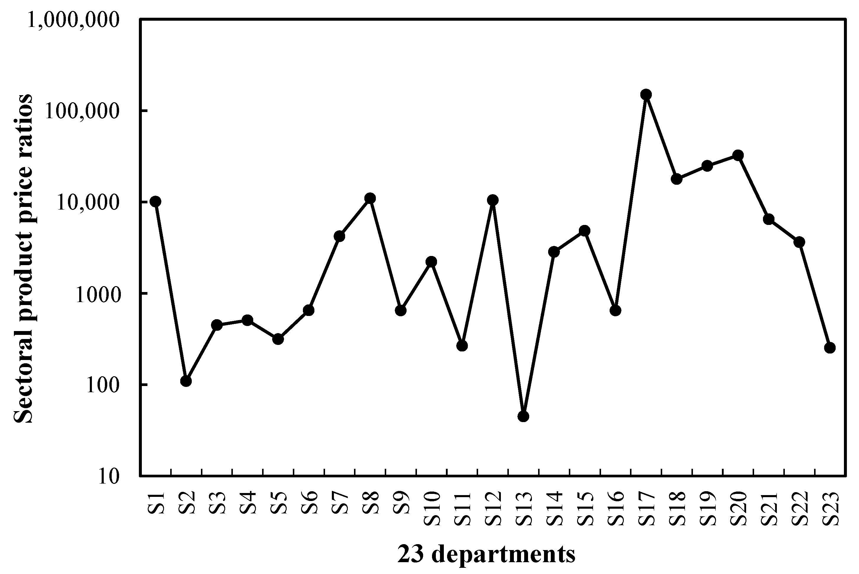
Economic data. We used data on the quantity and value of the main import and export of goods from the 2017 China Statistical Yearbook to calculate the product price ratio for the 23 sectors in the model. Subsequently, data related to the GDP and the structure of the three levels of industries in each of China’s 31 provinces from 2012 to 2020 were incorporated into our freight volume model. These data were also obtained from the China Statistical Yearbook [43].

2.2. Methodology

The Input–Output tables offer insights into the economic correlations between the 42 sectors of the regional economy. The inter-regional input–output tables, constructed using inter-regional trade data, are based on numerous regional input–output tables and reflect the input and output links between regional sectors and the direction of inter-regional freight flow. In this study, all inter-regional input–output tables pertained to the intermediate input matrix embedded in the inter-regional input–output tables, showcasing each sector’s value flow for each province.

Drawing from the inter-regional freight exchange volume data for public roads, railways, and waterways in 2017, we devised a freight volume forecasting model grounded in the input–output model. This involved the computation of coefficients for inter-regional trade, direct consumption and inter-regional price disparity. The GDP of each province and the ratio of the three levels of industries in the future were incorporated into the model to simulate inter-regional freight volume in subsequent years. The total input of each sector in each province was calculated to derive the future inter-regional input–output tables, which were then transmuted into the inter-regional freight volume for subsequent years. The method for constructing the freight volume model is depicted in Figure 1.

2.2.1. Creating Inter-Regional Input–Output Tables

(1)

Basic Principles

An inter-regional input–output model is established based on the input–output table and the input–output balanced. The main types of models are the row coefficient, column coefficient, and gravity models. The empirical analysis of Polensk’s (1970) three inter-regional input–output models revealed that the column coefficient model has low information requirements and a high simulation accuracy. Moses (1995) proposed an input–output balance for the column coefficient model with the following matrix form:

$$X=CAX+CF+E - M$$

(1)

where X is the total output of each region, F is the final demand of each region, and E and M are the exports and imports of each region, respectively. These variables are known and can be directly obtained from the input–output table of the 31 provinces in China. A is the direct consumption coefficient matrix calculated from the input–output table. C is the inter-regional trade coefficient matrix, which should be calculated in the subsequent research. CAX is the intermediate input matrix of the inter-regional input–output table.

(2)

Direct consumption factor matrix

A is a block diagonal matrix composed of the direct consumption coefficient matrix of 31 areas, each comprising of a 42 × 42 square matrix. The calculation formula of the direct consumption coefficient is as follows:

$$a_{ij}=\frac{x_{ij}}{X_j}$$

(2)

where a_ij represents the direct consumption coefficient of sector j to sector i, x_ij is the value of the goods or services of the product sector i directly consumed by the product sector j, X_j is the total output of the product sector j.

(3)

Inter-regional trade coefficient matrix

The inter-regional trade coefficient matrix C comprises of a diagonal matrix; the calculation formula for the element c_i^RS on the diagonal is as follows:

$$c_i^{RS }=\frac{t_i^{RS}}{{{\displaystyle \sum }}_{R=1}^m{t}_i^{RS}}$$

(3)

where t_i^RS is the number of products i supplied by region R to region S—that is, inter-regional trade flow, which can be calculated using the gravity model proposed by Leontief and Strout (1961); the calculation formula is as follows:

$$t_i^{RS}=\frac{x_i^R{d}_i^S}{{{\displaystyle \sum }}_{R=1}^m{x}_i^R}{Q}_i^{RS}$$

(4)

where x_i^R is the total output (total supply) of sector i in the region R, d_i^S is the total demand for the product of sector i in the region S (the sum of the intermediate demand and final demand). Q_i^RS is the product of sector i from the region R to the region S. The trade parameter is referred to as the friction coefficient. Ihara (1979) assumed that the ratio of the amount of material transported from one area to another is similar to the distribution ratio of the most important products; the calculation formula is as follows:

$$Q_i^{RS}=\frac{H_i^{RS}}{\frac{H_i^{RO}{H}_i^{OS}}{H_i^{\infty }}}$$

(5)

where H_i^RS is the freight volume sent from area R to area S, H_i^RO is the total freight volume sent from area R to all provinces, H_i^OS is the total freight volume reaching area S, and H_i^OO is the total shipment volume from all areas (equal to the total arrival).

The provincial GDP and radio of the three major industries’ levels were input. The total inputs for each province and sector were calculated based on the added-value coefficients, which produced inter-regional input–output tables based on the inter-regional matrix of direct consumption coefficients.

2.2.2. Converting Input–Output Table Values to Freight Volumes

A correlation between freight and value flows was established based on the sectoral product prices. We converted the value flows between 23 sectors into freight flows based of the following formula: flow/price = freight flow. This conversion facilitated the transformation of the inter-regional input–output tables into inter-provincial freight OD (origin-destination) tables for China’s 31 provinces.

However, only a portion of the 42 sectors included in the inter-regional input–output table engaged in the production of goods for transportation. For instance, the coal mining sector produces coal, and the oil and gas extraction sector produces oil. In contrast, certain sectors, such as education and finance, do not yield corresponding transportable products. As such, these sectors that do not produce transport goods must be excluded from the value-to-freight conversion calculation in the inter-regional Input–Output tables. The final inter-regional value flow to freight flow conversion retained only the top 23 sectors that generate freight demand. Among these 23 retained sectors, the first sector represented primary industries, while the remaining 22 sectors represented secondary industry.

Two key factors affected sectoral product prices: (1) the price variances among the 23 sectors within a single province and (2) the price discrepancies within the same sector across the 31 provinces and cities, stemming from uneven economic development between provinces. This is referred to as the regional price inhomogeneity coefficient. The unit prices of products within the 23 sectors were calculated based on the volume and value of the main goods imported and exported in 2017 and were considered as price ratios. The regional price inhomogeneity coefficients for each province were ascertained based on the total output value and goods dispatched by that province in 2017.

3. Freight Volume Model Based on Inter-Regional Input–Output Table Model

3.1. Creating Inter-Regional Input–Output Tables Model

The inter-regional freight exchange volume in 2017 was amplified by the year-on-year increase in the ratio of road and waterway freight volume in 2017 and 2008, and the railway freight exchange volume was obtained by the year-on-year increase in the proportion of railway freight volume in 2017 and 2012. From this, the combined inter-regional freight exchange volume for the roads, railways, and waterways in 2017 was obtained. The sent volume and arrival volume of the roadways, railways, and waterways in the 31 provinces of China in 2017 are shown in Figure 2. With the evolution of our economy, the developmental landscapes and models of different regions have changed accordingly. Different regions presented different demands for freight transportation. In 2017, North, South, and East China exhibited the highest freight exchange volume, averaging 6 billion tons, followed by Central Northeast and South China at 4 billion tons. However, Southwest and Northwest China, impacted by weaker industrial bases and inferior transportation, registered an average freight exchange volume of only about 1 billion tons.

The friction coefficient was calculated using Equation (5) based on the total inter-regional freight exchange volume in 2017. The trend of the variation in the friction coefficient with distance for the 31 provinces of China is shown in Figure 3.

The figure above showed that the friction coefficient decreases with an increase in distance. The slope values of the trend line were calculated to further investigate their relationship between trend lines, as shown in Figure 4.

The above figure illustrated that the friction coefficient and the slope of the distance trend line calculated from the total send volume for roadways, railways, and waterways were more concentrated, and the effect was improved. Therefore, in Equation (5), the friction coefficient, calculated based on the total freight volume sent by roadways, railways, and waterways, had the strongest correlation with distance, and this result was the most reasonable.

Following previous research on methods for constructing the inter-regional input–output tables, the final inter-regional input–output table was calculated and constructed based on the GDP of each region and the added value ratio of each department of 42 sectors in the base year. However, the model only considered the value of the three industries in the base year when using this method to create the inter-regional input–output table. China’s industrial structure is constantly changing based on its current economic development pattern. Therefore, when building the model, the input value was translated into the GDP value and the proportion value of the three industries of each region in order to eliminate the influence of the industrial structure on the freight volume. Next, the model prepared the inter-regional input–output table. The developed model could quantify the degree to which changes in the industrial structure of each region impacted the estimated value of the inter-regional freight volume.

3.2. Converting Input–Output Table Values to the Freight Volume Model

When calculating the sectoral prices, it was necessary to classify the goods according to their sectors based on the main goods imported and exported in 2017 before calculating the unit prices of these goods separately and averaging them as the product prices of the whole sector. In this way, we determined the 23 sectoral product prices, which were considered price ratios. The regional prices for each province could then be determined based on the total value output and total goods exported in 2017. The price heterogeneity coefficient for each area was subsequently determined based on the total output value and goods exported in 2017.

The 23 sectoral product price ratios are shown in Figure 5, and the inter-regional price unevenness coefficient is shown in Figure 6.

The findings demonstrated that the product price ratio of specialized equipment, electrical machinery, communications equipment, and other high-value-added sectoral products were more significant. Conversely, the coal mining products, non-metallic mineral products, scrap waste, and low-value-added sectoral product price ratios were less substantial.

According to the above parameters, the calculated and measured values of the total freight transport in the 31 provinces of China in 2017 are compared in Figure 7. The comparison of the calculated and measured values of sending and arriving volumes in the 31 provinces of China in 2017 are shown in Figure 8. The calculation results showed that the determined coefficient values of the measured and calculated sending-and-arriving volumes of the 31 provinces in China were between 0.9 and 1.

The simulation results demonstrate a strong model fit and suitable model rate parameters.

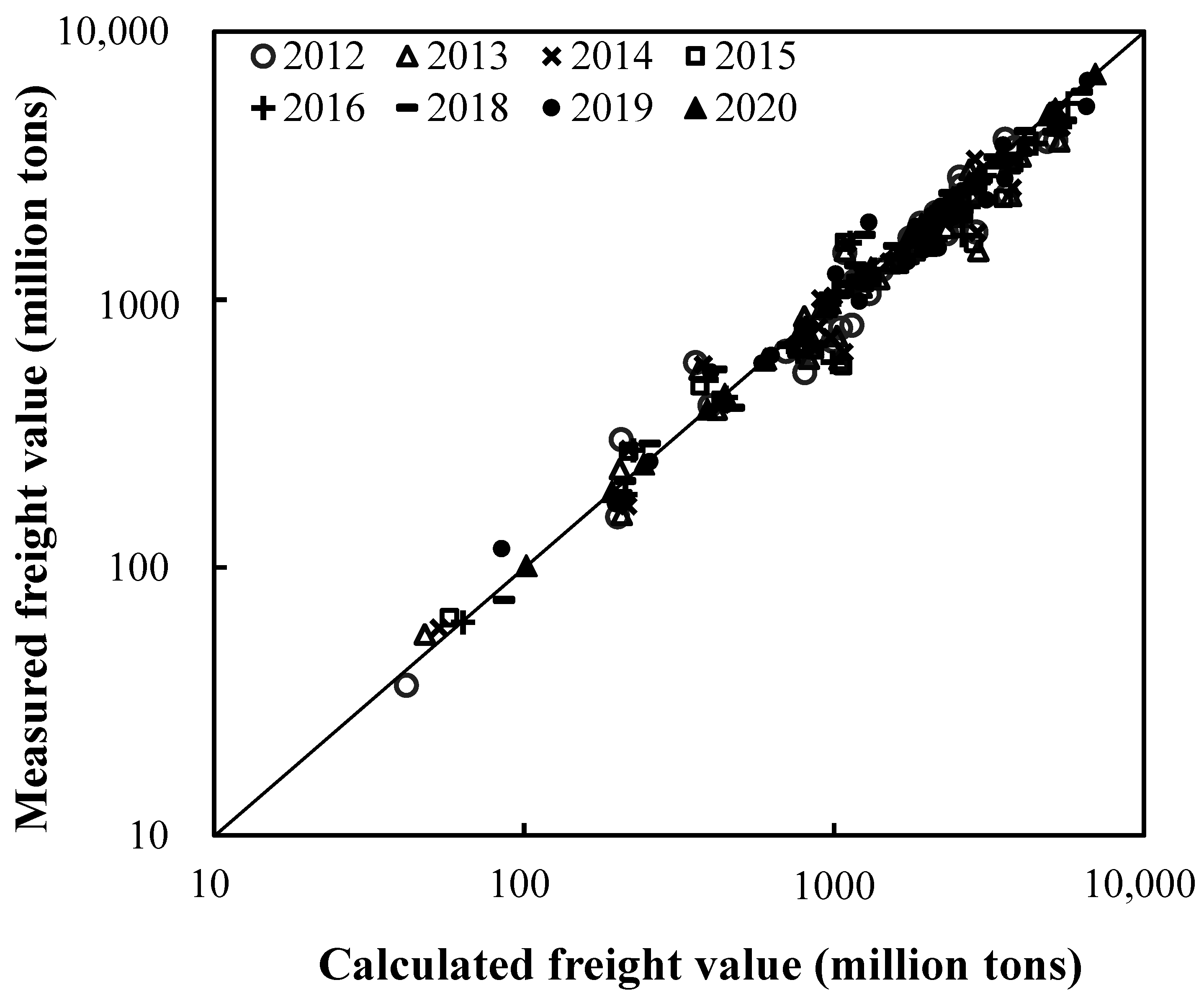
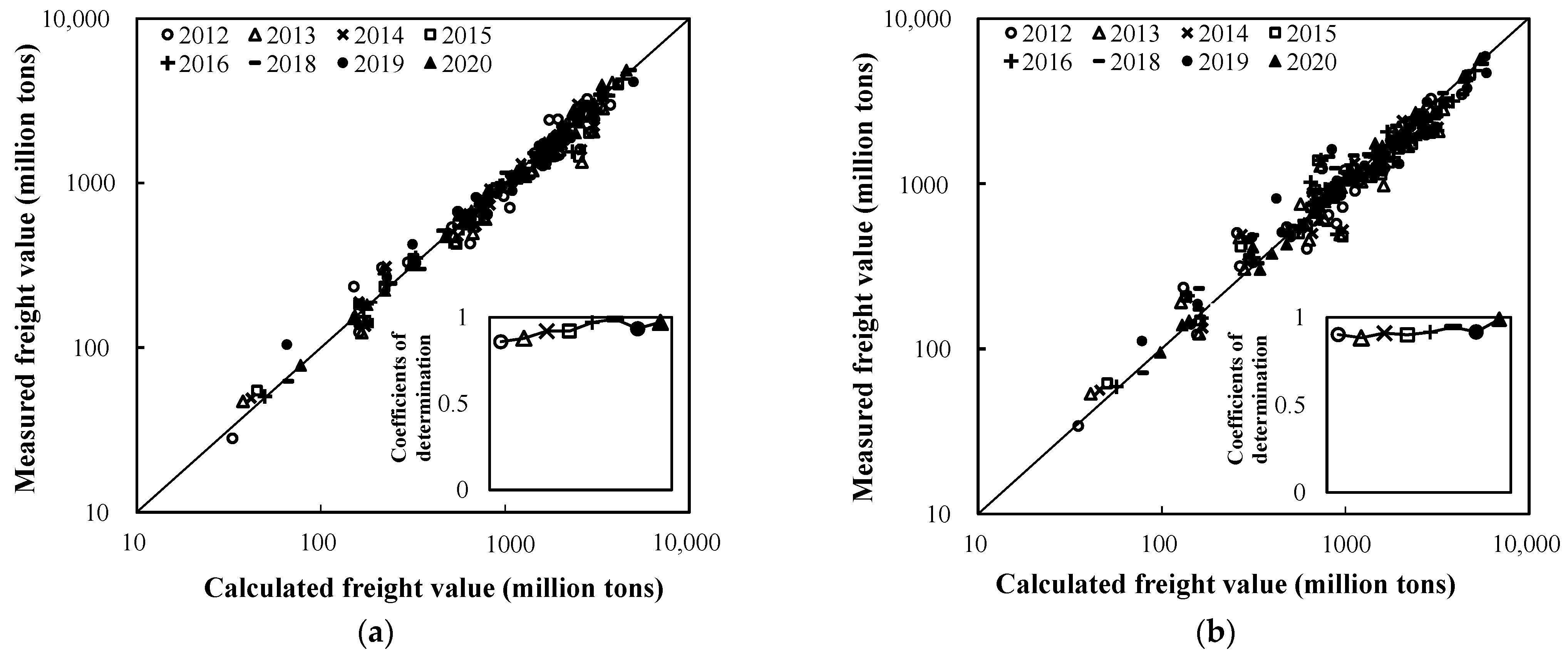
3.3. Model Validation

The model employed the simulated total freight and freight flows from 2012 to 2016 and 2018 to 2020 for validation. The input variables included the GDP and the proportion of the three industries’ levels in each province. The inter-regional input–output table was then calculated based on the inter-regional direct consumption coefficient matrix and the GDP’s sectoral distribution, after which the volume was transformed into freight volume.

Using the model for computation, the total send-and-arrival volume was considered as the total freight volume. The measured and calculated values of the total freight volume of the 31 Chinese provinces and their determination coefficients from 2012 to 2016 and from 2018 to 2020 are shown in Figure 9. The comparison between the calculated and measured values of the total send volume and the total arrival volume of these 31 provinces and their determination coefficients are shown in Figure 10.

The results showed that the simulation of the freight volume for the Chinese provinces was accurate, and the closer to 2017, the more effective the simulation.

4. Discussion

Given that the inter-regional freight volume reflects the inter-regional economic exchanges and acts as a basis for transportation infrastructure planning decisions, simulating the inter-regional freight volumes is crucial.

We employed the inter-regional input–output tables and considered changes in the GDP and industrial structure to address the deficiencies in simulating China’s inter-regional freight volume. A regional freight volume forecasting model was then built to assess the impact of industrial structure changes on freight demand. The relationship between the GDP and freight volume in China from 1985 to 2020 is shown in Figure 11. GDP and freight volume were positively correlated. The trend line in the figure indicated that as the GDP grew, the rate of increase in freight volume slowed and eventually plateaued.

To further examine the relationship between the three levels of industries and freight volume, we introduced two indicators: the industrial structure coefficient and freight intensity. The industrial structure coefficient was obtained by dividing the added value of the tertiary industry by the sum of the added value of the primary and the secondary industry. Freight intensity was defined as the freight volume generated per unit GDP, calculated as follows:

$$freight intensity=\frac{freight volume}{GDP}$$

(6)

The change in industrial structure coefficient and freight volume from 1985 to 2020 is shown in Figure 12. The industrial structure coefficient had been on the rise for many years, increasing slowly before 2010, and then rapidly after 2010. Additionally, an upward tendency in the overall freight volume was observed, with a sluggish increase before 2005, a rapid increase after 2005, and a high value in 2018.

To further investigate the relationship between the freight intensity and industrial structure, the proportion of the three industries’ levels in 2017 was used as the benchmark value for parameter calculation. The following conditions were set under the premise that the GDP remained constant and the proportion of the three industries’ levels are 1, the influence of the change in the proportion of the three industries’ levels input by the model on the calculated freight volume was verified. This could be broken down into the six cases in

Table 1. Changes in the three industries in six cases.

Different Cases	The Primary Sector	The Secondary Sector	The Secondary Sector
Benchmark value	7.4%	39.9%	52.7%
Case 1	7.4%	69.9% (30% increased)	22.7% (30% decreased)
Case 2	7.4%	59.9% (20% increased)	32.7% (20% decreased)
Case 3	7.4%	49.9% (10% increased)	42.7% (10% decreased)
Case 4	7.4%	29.9% (10% decreased)	62.7% (10% increased)
Case 5	7.4%	19.5% (20% decreased)	72.7% (20% increased)
Case 6	7.4%	9.5% (30% decreased)	82.7% (30% increased)

.

Based on the output value of the three industry sectors in the above six cases, the inter-regional input–output model was used to simulate the freight volume. The relationship between China’s freight intensity and industrial structure coefficient under six cases are shown in Figure 13.

An observable rule governed the relationship curve between the freight intensity and industrial structure coefficient calculated from the real-world data. As the industrial structure coefficient increased, the freight intensity showed a downward trend, indicating a negative correlation. This trend could be split into two phases. In the first phase, the freight intensity dropped sharply. In the second phase, when the industrial structure coefficient reached a certain range, the freight intensity decreased slowly, even stabilizing. Moreover, the trend line representing the data calculated with the model parameters closely mirrored the trend line of the actual data. This correlation indicated a superior simulation effect compared to data calculated without considering the model parameters. Finally, the trend lines of the calculated and actual data intersected when the x-axis value equaled 0.795. When the x-axis value was less than 0.795, the two trend lines were distant, and so the model did not accurately simulate the impact of the industrial structure on the freight volume. Conversely, when the x-axis value was above 0.795, the two trend lines were very close, and so the simulation of the model was effective.

In summary, we could establish the following:

(1)

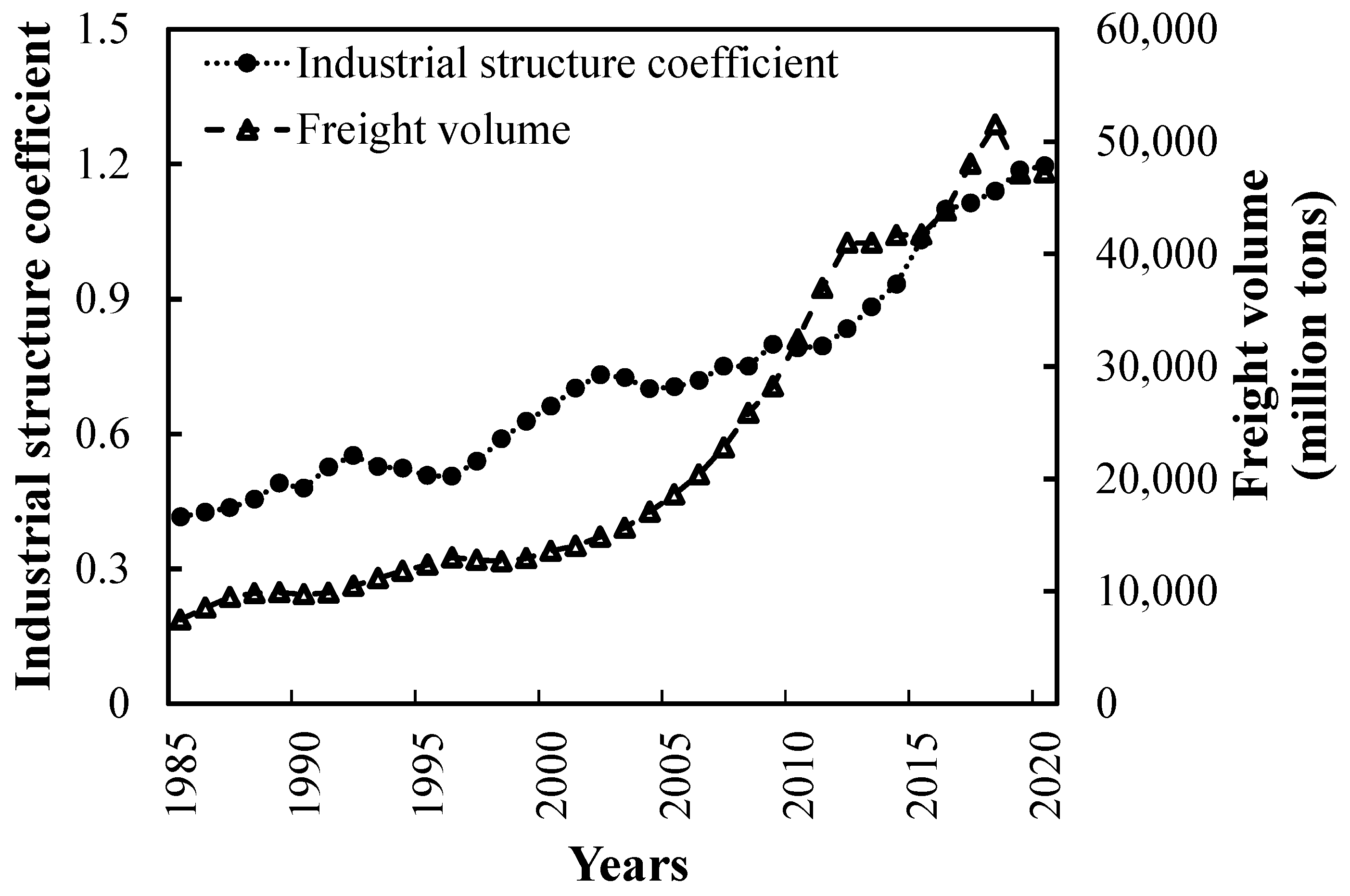
Only the first 23 sectors in the input–output table that resulted in freight exchanges were retained when the model was used to convert value into freight volume. These sectors belonged to the primary and secondary industry levels. Hence, the annual changes in the industrial structure should also be considered when determining the freight volume.

(2)

The model primarily used price to establish the relationship between value and freight volume. Therefore, it is important to consider not just the departmental pricing in a given year, but also the price changes for products across sectors over time and the impact of inflation.

5. Conclusions

Since the inter-regional freight volume physically represents inter-regional economic exchange and underpins transportation infrastructure planning, the precise estimation of inter-regional freight demand is crucial. This study established a simulation model for the inter-regional freight volume based on the input–output tables of 42 sectors in the 31 provinces of China. The model converted the inter-regional value flow into freight flow using product prices and revealed the impact of changes in the industrial structure on freight demand. The primary conclusions were as follows:

(1)

An inter-regional freight volume forecasting model for China was developed based on the principles of the IO and the creation of inter-regional input–output tables derived from the corresponding tables of each province. This model calculated the impact of changes in the industrial structure on the freight volume simulations and determined the overall freight demand across regions, which could inform transportation infrastructure planning.

(2)

Converting the value into freight volume using the inter-regional input–output table required calculations based on department prices. However, each sector’s product quantity and value data were incomplete. The product price primarily relied on base year data, while data for other years were determined by the price and inflation rate of the base year, reducing the model’s calculation accuracy. The model was more accurate for predicting freight volume for the next five years due to inflation.

(3)

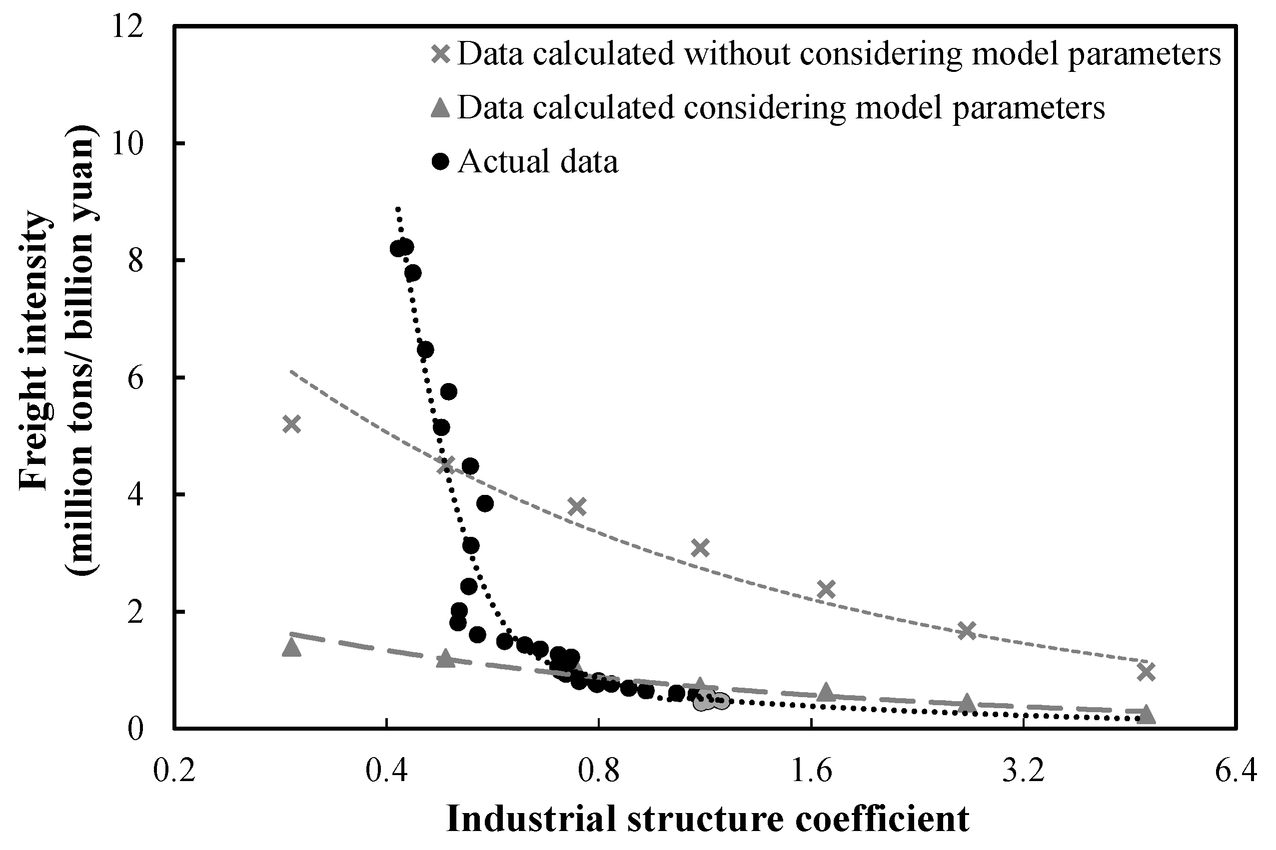
We performed a quantitative analysis of the forecasting results of the inter-regional freight volume model, examining the effects of changes in the structural makeup of the three industries. This research showed that the contribution of tertiary industries to the freight volume is relatively small. When the proportion of tertiary industries increased and the proportion of primary and secondary industries decreased, the freight intensity slowly declined and finally reached stability.

References

1. Huo, Z.; Zha, X.; Lu, M.; Ma, T.; Lu, Z. Prediction of Carbon Emission of the Transportation Sector in Jiangsu Province-Regression Prediction Model Based on GA-SVM. Sustainability 2023, 15, 3631. [Google Scholar] [CrossRef]
2. Jin, G.; Feng, W.; Meng, Q. Prediction of Waterway Cargo Transportation Volume to Support Maritime Transportation Systems Based on GA-BP Neural Network Optimization. Sustainability 2022, 14, 13872. [Google Scholar] [CrossRef]
3. Xu, X.; Chase, N.; Peng, T. Economic structural change and freight transport demand in China. Energy Policy 2021, 158, 112567. [Google Scholar] [CrossRef]
4. Davydenko, I.Y.; Tavasszy, L.A. Estimation of Warehouse Throughput in Freight Transport Demand Model for the Netherlands. Transp. Res. Rec. 2013, 2379, 9–17. [Google Scholar] [CrossRef]
5. Lu, B.; Wang, S.Y.; Kuang, H.B. Research on regional logistics demands forecasts based on the gravity model. Manag. Rev. 2017, 29, 181–190. (In Chinese) [Google Scholar] [CrossRef]
6. Li, B.; Gao, S.; Liang, Y.; Kang, Y.; Prestby, T.; Gao, Y.; Xiao, R. Estimation of Regional Economic Development Indicator from Transportation Network Analytics. Sci. Rep. 2020, 10, 2647. [Google Scholar] [CrossRef] [PubMed] [Green Version]
7. Rubio-Herrero, J.; Muñuzuri, J. Indirect estimation of interregional freight flows with a real-valued genetic algorithm. Transportation 2021, 48, 257–282. [Google Scholar] [CrossRef]
8. Shen, L.; Shao, Z.; Yu, Y.; Chen, X. Hybrid Approach Combining Modified Gravity Model and Deep Learning for Short-Term Forecasting of Metro Transit Passenger Flows. Transp. Res. Rec. 2020, 2675, 25–38. [Google Scholar] [CrossRef]
9. Shang, Q.; Deng, Y.; Cheong, K.H. Identifying influential nodes in complex networks: Effective distance gravity model. Inf. Sci. 2021, 577, 162–179. [Google Scholar] [CrossRef]
10. Gragera, A.; Hybel, J.; Madsen, E.; Mulalic, I. A model for estimation of the demand for on-street parking. Econ. Transp. 2021, 28, 100231. [Google Scholar] [CrossRef]
11. Aksenov, G.; Li, R.; Abbas, Q.; Fambo, H.; Popkov, S.; Ponkratov, V.; Kosov, M.; Elyakova, I.; Vasiljeva, M. Development of Trade and Financial-Economical Relationships between China and Russia: A Study Based on the Trade Gravity Model. Sustainability 2023, 15, 6099. [Google Scholar] [CrossRef]
12. Li, J.; Zheng, P.Q. Construction and application of entropy change model of public transit commuting based on IC card data. Transp. Syst. Eng. Inf. 2020, 20, 234–240. (In Chinese) [Google Scholar] [CrossRef]
13. Huang, T.; Kockelman, K.M. The introduction of dynamic features in a random-utility-based multi-regional input-output model of trade, production, and location choice. J. Transp. Res. Forum 2010, 47, 206900. [Google Scholar] [CrossRef]
14. Mizutani, M.; Tsuchiya, K.; Takuma, F.; Ohashi, T. Estimation of the economic benefits of port development on international maritime market by partial equilibrium model and SCGE model. J. East. Asia Soc. Transp. Stud. 2005, 6, 892–906. [Google Scholar] [CrossRef]
15. Zhang, J.; Chang, Y.; Wang, C.; Zhang, L. The green efficiency of industrial sectors in China: A comparative analysis based on sectoral and supply-chain quantifications. Resour. Conserv. Recycl. 2018, 132, 269–277. [Google Scholar] [CrossRef]
16. Anas, A.; De Sarkar, S.; Timilsina, G.R. Bus Rapid Transit versus road expansion to alleviate congestion: A general equilibrium comparison. Econ. Transp. 2021, 26–27, 100220. [Google Scholar] [CrossRef]
17. Shibasaki, R.; Watanabe, T. Future Forecast of Trade Amount and International Cargo Flow in the APEC Region: An Application of Trade-Logistics Forecasting Model. Asian Transp. Stud. 2012, 2, 194–208. [Google Scholar] [CrossRef]
18. Ma, M.; Huang, D.; Hossain, S.S. Opportunities or Risks: Economic Impacts of Climate Change on Crop Structure Adjustment in Ecologically Vulnerable Regions in China. Sustainability 2023, 15, 6211. [Google Scholar] [CrossRef]
19. Chan, Y.T.; Dong, Y. How does oil price volatility affect unemployment rates? A dynamic stochastic general equilibrium model. Econ. Model. 2022, 114, 105935. [Google Scholar] [CrossRef]
20. Chan, Y.T.; Zhao, H. Optimal carbon tax rates in a dynamic stochastic general equilibrium model with a supply chain. Econ. Model. 2023, 119, 106109. [Google Scholar] [CrossRef]
21. Yoshino, N.; Rasoulinezhad, E.; Taghizadeh-Hesary, F. Economic impacts of carbon tax in a general equilibrium framework: Empirical study of Japan. J. Environ. Assess. Policy Manag. 2021, 23, 2250014. [Google Scholar] [CrossRef]
22. Itskhoki, O.; Mukhin, D. Exchange rate disconnect in general equilibrium. J. Politi Econ. 2021, 129, 2183–2232. [Google Scholar] [CrossRef]
23. Di Pietro, F.; Lecca, P.; Salotti, S. Regional economic resilience in the European Union: A numerical general equilibrium analysis. Spat. Econ. Anal. 2020, 16, 287–312. [Google Scholar] [CrossRef]
24. Cao, J.; Dai, H.; Li, S.; Guo, C.; Ho, M.; Cai, W.; He, J.; Huang, H.; Li, J.; Liu, Y.; et al. The general equilibrium impacts of carbon tax policy in China: A multi-model comparison. Energy Econ. 2021, 99, 105284. [Google Scholar] [CrossRef]
25. Marshall, E.C.; Saunoris, J.; Solis-Garcia, M.; Do, T. Measuring the size and dynamics of U.S. state-level shadow economies using a dynamic general equilibrium model with trends. J. Macroecon. 2023, 75, 103491. [Google Scholar] [CrossRef]
26. Shao, G.; Miller, R.E. Demand-side and supply-side commodity-industry multiregional input–output models and spatial linkages in the US regional economy. Econ. Syst. Res. 1990, 2, 385–406. [Google Scholar] [CrossRef]
27. Cascetta, E.; Marzano, V.; Papola, A. Multi-Regional Input-Output Models for Freight Demand Simulation at a National Level. Recent Developments in Transport Modelling; Emerald Group Publishing Limited: City of Bradford, UK, 2008; pp. 93–116. [Google Scholar] [CrossRef]
28. Alises, A.; Vassallo, J.M. The impact of the structure of the economy on the evolution of road freight transport: A macro analysis from an input-output approach. Transp. Res. Procedia 2016, 14, 2870–2879. [Google Scholar] [CrossRef] [Green Version]
29. Pompigna, A.; Mauro, R. Input/Output models for freight transport demand: A macro approach to traffic analysis for a freight corridor. Arch. Transp. 2020, 54, 21–42. [Google Scholar] [CrossRef]
30. Leurent, F.; Windisch, E. Benefits and costs of electric vehicles for the public finances: An integrated valuation model based on input–output analysis, with application to France. Res. Transp. Econ. 2015, 50, 51–62. [Google Scholar] [CrossRef]
31. Pang, J.; Gao, X.M.; Shi, Y.C. Effect of Energy resource Tax Reform on Income Distribution of Chinese urban residents: An Analysis based on Input-output model. China Environ. Sci. 2019, 6, 402–411. (In Chinese) [Google Scholar] [CrossRef]
32. Han, Y.; Lou, X.; Feng, M.; Geng, Z.; Chen, L.; Ping, W.; Lu, G. Energy consumption analysis and saving of buildings based on static and dynamic input-output models. Energy 2021, 239, 122240. [Google Scholar] [CrossRef]
33. Sun, C.; Chen, Z.; Guo, Z.; Wu, H. Energy rebound effect of various industries in China: Based on hybrid energy input-output model. Energy 2022, 261, 125147. [Google Scholar] [CrossRef]
34. Yang, Y.; Park, Y.; Smith, T.M.; Kim, T.; Park, H.-S. High-Resolution Environmentally Extended Input–Output Model to Assess the Greenhouse Gas Impact of Electronics in South Korea. Environ. Sci. Technol. 2022, 56, 2107–2114. [Google Scholar] [CrossRef] [PubMed]
35. Sarkar, B.D.; Shankar, R.; Kar, A.K. A scenario-based interval-input output model to analyze the risk of COVID-19 pandemic in port logistics. J. Model. Manag. 2021, 17, 1456–1480. [Google Scholar] [CrossRef]
36. Fu, R.; Jin, G.; Chen, J.; Ye, Y. The effects of poverty alleviation investment on carbon emissions in China based on the multiregional input–output model. Technol. Forecast. Soc. Chang. 2021, 162, 120344. [Google Scholar] [CrossRef]
37. Zhao, J.; Zhou, S.; Cui, X.; Wang, G. Road freight volume forecasting method based on fuzzy linear regression model. J. Traffic Transp. Eng. 2012, 12, 80–85. (In Chinese) [Google Scholar] [CrossRef]
38. Wu, Z.D.; Zhao, M.; Ma, C. A study of inter-provincial trade estimation based on input-output tables. Stat. Decis. 2014, 10, 293. (In Chinese) [Google Scholar] [CrossRef]
39. Yu, Y. Re-estimation and interval decomposition of inter-provincial trade flows in China. China Econ. Stud. 2013, 5, 100–108. (In Chinese) [Google Scholar]
40. Mi, Z.; Meng, J.; Zheng, H.; Shan, Y. A multi-regional input-output table mapping China’s economic outputs and interdependencies in 2012. Sci. Data 2018, 5, 180155. [Google Scholar] [CrossRef] [PubMed] [Green Version]
41. Input Output Table of China Region–2017. Available online: https://data.stats.gov.cn/ifnormal.htm?u=/files/html/quickSearch/trcc/trcc01.html&h=740&from=groupmessage&isappinstalled=0 (accessed on 30 December 2022). (In Chinese)
42. China Traffic Yearbook. Available online: http://libvpn.cqjtu.edu.cn/rwt/CNKI/https/MSRYIZJPMNYGX4JPN3TYE/yearBook/single?id=N2010080093 (accessed on 25 December 2022). (In Chinese)
43. China Statistical Yearbook. Available online: http://www.stats.gov.cn/tjsj/ndsj/ (accessed on 10 December 2022). (In Chinese)
Figure 1. The construction process of the freight volume model.
Sustainability 15 09808 g001
Figure 2. The total sent volume and arrival volume of roadways, railways, and waterways in the 31 provinces in China in 2017.
Sustainability 15 09808 g002
Figure 3. (a) The trend line of the friction coefficient with distance calculated from the total send volume of roadways, railways, and waterways; (b) The trend line of the friction coefficient with distance calculated from the send volume of railways.
Sustainability 15 09808 g003
Figure 4. Distribution of the slope value of the trend line of the friction coefficient with distance.
Sustainability 15 09808 g004
Figure 5. The product price ratio of 23 departments.
Sustainability 15 09808 g005
Figure 6. Inter-regional price unevenness coefficient.
Sustainability 15 09808 g006
Figure 7. Comparison between the calculated and measured values of the total freight volume of each province in 2017.
Sustainability 15 09808 g007
Figure 8. Comparison of the calculated and measured values of the send-and-arrival volume in the 31 provinces of China in 2017.
Sustainability 15 09808 g008
Figure 9. Comparison of the calculated and measured values of the total freight volume of the 31 provinces in China and their determination coefficients.
Sustainability 15 09808 g009
Figure 10. (a) Comparison of calculated and measured values of the total send volume and their determination coefficients; (b) comparison of calculated and measured values of the total arrival volume and their determination coefficients.
Sustainability 15 09808 g010
Figure 11. The relationship between the GDP and freight volume in China from 1985 to 2020.
Sustainability 15 09808 g011
Figure 12. Change of industrial structure coefficient and freight volume from 1985 to 2020.
Sustainability 15 09808 g012
Figure 13. The relationship between China’s freight intensity and the industrial structure coefficient under six cases.
Sustainability 15 09808 g013