Article

Optimizing Regression Models for Predicting Noise Pollution Caused by Road Traffic

by
Amal A. Al-Shargabi
1,
Abdulbasit Almhafdy
2,*,
Saleem S. AlSaleem
3,
Umberto Berardi
4 and
Ahmed AbdelMonteleb M. Ali
2,5
1
Department of Information Technology, College of Computer, Qassim University, Buraydah 52571, Saudi Arabia
2
Department of Architecture, College of Architecture and Planning, Qassim University, Buraydah 52571, Saudi Arabia
3
Department of Civil Engineering, College of Engineering, Qassim University, Buraydah 52571, Saudi Arabia
4
Department of Architectural Science, Faculty of Engineering and Architectural Science, Toronto Metropolitan University, 325 Church Street, Toronto, ON M5B 2K3, Canada
5
Department of Architectural Engineering, Faculty of Engineering, Assiut University, Assiut 71515, Egypt
*
Author to whom correspondence should be addressed.
Sustainability 2023, 15(13), 10020; https://doi.org/10.3390/su151310020
Submission received: 3 May 2023 / Revised: 19 June 2023 / Accepted: 20 June 2023 / Published: 25 June 2023
(This article belongs to the Section Pollution Prevention, Mitigation and Sustainability)

Abstract

:
The study focuses on addressing the growing concern of noise pollution resulting from increased transportation. Effective strategies are necessary to mitigate the impact of noise pollution. The study utilizes noise regression models to estimate road-traffic-induced noise pollution. However, the availability and reliability of such models can be limited. To enhance the accuracy of predictions, optimization techniques are employed. A dataset encompassing various landscape configurations is generated, and three regression models (regression tree, support vector machines, and Gaussian process regression) are constructed for noise-pollution prediction. Optimization is performed by fine-tuning hyperparameters for each model. Performance measures such as mean square error (MSE), root mean square error (RMSE), and coefficient of determination (R2) are utilized to determine the optimal hyperparameter values. The results demonstrate that the optimization process significantly improves the models’ performance. The optimized Gaussian process regression model exhibits the highest prediction accuracy, with an MSE of 0.19, RMSE of 0.04, and R2 reaching 1. However, this model is comparatively slower in terms of computation speed. The study provides valuable insights for developing effective solutions and action plans to mitigate the adverse effects of noise pollution.

1. Introduction

The increasing demand for trips and transportation has resulted in significant challenges in terms of traffic congestion and safety, which can have a negative impact on economic growth and quality of life [1]. To address these issues and provide a better transportation experience for citizens, accurate data about traffic noise is critical for the effective management of traffic, as well as for the overall health and well-being of communities. With accurate and up-to-date information about traffic-noise levels, cities and urban areas can develop more efficient transportation systems and create better living environments for their citizens [1].
Noise pollution, particularly from road traffic, is a widespread and complex issue in urban environments. According to De Coensel, Brown, and Tomerini [2], the frequency, duration, and intensity of noise events from road traffic can contribute to noise annoyance levels. It is, therefore, critical to consider road traffic as a source of noise pollution and to implement measures to reduce its impact [3,4]. The negative effects of noise pollution on physical health [5], well-being [6], and even mortality [7], are widely recognized. Excessive noise exposure at home, school, work, and other settings can disrupt concurrent activities and performance and may also have long-term effects on human health and development [8].
Developing effective traffic-control strategies to reduce the impact of road traffic on the community requires comprehensive and accurate road-traffic state data, while evaluating the noise pollution caused by road traffic is crucial to assess the environmental quality of urban areas and the well-being of their residents [1]. Accurate measurement and analysis of noise events can inform the development of effective noise-reduction strategies, such as noise barriers, traffic-management techniques, and regulation of vehicle emissions [1]. These efforts can lead to a variety of benefits, including improved quality of life for residents, reduced stress and health problems, and a more sustainable urban environment.
Urban noise levels have been classified according to traffic composition for environmental noise assessment [9]. Using expert systems and artificial intelligence (AI), the study demonstrated the potential of AI applications in assessing noise-pollution problems and gathering information for more informed action against urban traffic noise. According to Botteldooren et al. [10], instead of finding an accurate and precise prediction, noise-prediction models should identify a fuzzy set of possibilities. To calculate predictions more specific for small groups of individuals, a few typical rules were derived from empirical knowledge. The novel noise-effect-modeling approach was tested in practice and used as an advisor for noise-nuisance management and to test hypotheses such as noise sensitivity and urbanization in social science.
Several studies have used an artificial neural network to estimate noise levels based on road-traffic inputs. Fallah-Shorshani et al. [11] evaluated the performance of common traffic-noise models in Long Beach, California. The authors assessed the accuracy of the statistical land-use regression model, the extreme gradient-boosting machine-learning model (XGB), and a commercial noise model (CadnaA) by comparing their predictions to actual noise data. Their results indicated that XGB and CadnaA were the top-performing models, providing the most accurate traffic-noise estimates. The optimization of these models, alongside the validation against recorded data, highlights their potential as reliable approaches for traffic-noise prediction and management. According to Adulaimi et al. [12], random forests (RF) outperformed land-use regression (LUR) in noise estimation. Yin et al. [13] conducted a comparative analysis of various machine-learning algorithms for estimating noise, including linear regression and XGB. Based on their findings, they concluded that XGB outperformed the other algorithms in terms of precision. This underscores the potential of XGB as a reliable approach to noise estimation, particularly in contexts where high precision is critical.
Nourani, Gökçekuş, and Umar [14] conducted a study to improve the accuracy of predicting vehicular-traffic noise in Nicosia, North Cyprus, using artificial intelligence. By classifying the number of vehicles, the AI models performed better, with up to 29% improvement, by identifying the most relevant input parameters. The nonlinear ANFIS ensemble performed the best, with improvements of 11%, 19%, 21%, and 31% for the ANFIS, FFNN, SVR, and MLR models, respectively. The study proposed a method for predicting noise pollution in urban areas by combining feature selection and machine-learning regression techniques, resulting in an R2 of 0.94 and a MAE of 1.14 to 1.16 dBA by using WFS for feature selection and either SMO or GPR for regression.
Givargis and Karimi [15] proposed a neural-network model to forecast the hourly noise levels on roads in Tehran that are located within four meters of the edge. Data were collected from 50 sample sites near five roads in Tehran, selected from the UK calculation of road-traffic-noise method. A non-parametric test was used to assess the effectiveness of the model after splitting the data into a training set, a testing set, and a validation set. The results revealed that the neural-network approach was statistically valid for predicting traffic noise in Tehran. Xu et al. In [16] developed a novel deep-learning framework for estimating road-traffic state using graph embedding (GE) for detector selection and GAN for traffic-data generation. The comparison of the GE-GAN model with other models (KNN, BP, Deeptrend2.0, BGCP, and LSTM) demonstrated that the GE-GAN model outperformed the other models.
The current study explores the impact of various factors such as speed limits, presence of heavy vehicles, time of day, type of landscape barriers, road materials, and distance from the road to the receiver point on traffic noise in various urban configurations. By leveraging the power of machine learning, the study aims to predict the effect of traffic-noise pollution on a public park in the city of Buraydah.
To achieve this goal, a unique dataset was generated specifically for the study to predict the impact of traffic noise on the park. The study compared the results of three machine-learning algorithms for their accuracy in predicting traffic noise: fine tree, support vector machines (SVM), and Gaussian process regression (GPR). The models were optimized by fine-tuning various parameters to determine the optimal algorithm for traffic-noise prediction.
The main contributions of this study are:
  • The dataset generated in this study was specifically designed to predict noise-pollution levels in public parks. The researchers collected data on various landscape configurations within the parks, such as the presence of trees, water bodies, and built structures. These data were then used to predict the levels of noise pollution in the parks. The generated dataset is a valuable resource for future studies as it provides a comprehensive and diverse representation of public-park landscapes and the associated noise-pollution levels;
  • The hyperparameters in a machine-learning model are parameters that are set before training the model. They influence the learning process and can greatly affect the model’s performance. In this study, the researchers investigated different hyperparameter options to optimize the prediction models for noise pollution in public parks. This means that they tried various combinations of hyperparameters to determine which set of parameters produced the best results. By exploring different hyperparameter options, the researchers aimed to improve the accuracy of the noise-pollution predictions and to identify the optimal set of hyperparameters for this problem;
  • Optimized and non-optimized regression models for predicting noise pollution in public parks. Regression is a type of machine-learning algorithm that is used to predict numerical values. The non-optimized regression models were developed without adjusting the hyperparameters, while the optimized regression models were developed by adjusting the hyperparameters using the findings from the different hyperparameter options explored earlier in the study. The comparison of the performance of the optimized and non-optimized regression models provided valuable insights into the impact of hyperparameter tuning on the accuracy of the noise-pollution predictions.
The rest of this paper is structured in the following manner. In Section 2, the experimental work and the process of generating the dataset are explained in detail. Section 3 presents the experimental results and conducts a comparison of the performance of the regression models. In Section 4, the main findings are discussed, and Section 5 provides a conclusion to the paper.

2. Method

The purpose of this section is to outline the method used to collect the data and set the configurations needed to train and test the prediction models. This will involve the generation of the dataset, as well as the fine-tuning of the model parameters, to ensure the models are equipped with the information they need to accurately predict traffic noise.

2.1. Experimental Setup

For this study, the experimental work was carried out utilizing the deep-learning toolbox available in MATLAB R2020a. All experiments were performed on a computer system equipped with a GPU (NVIDIA GeForce RTX 2060 8 GB). The usage of a GPU allows for accelerated computations and efficient training of deep-learning models, enabling faster experimentation and analysis. The traffic-noise prediction model proposed in this study is based on the adaptations of existing simulation models used in previous research such as that presented by De Can et al. [17] and De Coensel et al. [2,18]. The road traffic is modeled in a microscopic manner, taking into account each individual vehicle’s movements. This approach allows for a full-scale simulation of road traffic, taking into consideration various factors such as the road network, properties of the vehicle fleet, landscape configuration, and aggregated traffic-demand data. The simulation provides a continuous stream of data on the position, speed, and acceleration of each vehicle, offering a comprehensive representation of road traffic.

2.2. Dataset Description

During this case study, simulations were conducted in order to examine the impact of accounting for realistic power distributions for vehicle noise on estimates of measures that characterize sound events. To achieve this goal, receiver points are set up along a conventional straight road which is considered a usual configuration in the city. A simulation network containing a single road segment with a length of 1300 m was constructed using the IMMI traffic-simulation software [19].
Several factors were taken into account when simulating the road traffic, including distance from the street to the receiver points, time of day (day and night), presence of landscape barriers (such as trees and walls), road-finishing surfaces, number of vehicles per hour, speed limit, and the ratio of heavy vehicles (as shown in Table 1). These factors were included as features in the study to accurately reflect the real-life traffic conditions.
For this study, the data must be statistically significant. Therefore, 18 receiver points were installed along three different roads to represent all the design features. A series of 6480 scenarios were generated by varying the above-mentioned variables, as shown in Figure 1a–c. ISO 9613-2 models are used to calculate vehicle-noise-emissions spectra for all simulation scenarios.
Following that, the level of noise was measured by a PCE-322A (the device is from PCE Instruments U.K. Ltd., Southampton, UK, calibrated by Anaum International Electronics LLC, Abu Dhabi, United Arab Emirates, and compatible with standard IEC61672-1 CLASS2) at various distances away from the edge of the road, specifically at 15 m, 30 m, 45 m, 60 m, 75 m, and 90 m. The noise levels are also measured at a height of 1.5 m from the ground, at receiver points located along the perpendicular bisector of the simulated road segment. These measurements are taken to provide a comprehensive understanding of the noise levels and their distribution in the area surrounding the road.

2.3. The Regression Models

As discussed previously, the aim of this study is to forecast the noise-pollution levels caused by road traffic by taking into account various predictors, such as the distance from the road to the receiver points, the time of day, the type of landscape barriers, the material of the road surface, the number of vehicles per hour, the speed limit, and the percentage of heavy vehicles. To accomplish this goal, the study employs and compares the results of three different regression models: fine tree, support vector machine (SVM), and Gaussian process regression (GPR).
In order to improve the performance of the models, optimization is utilized to optimize certain hyperparameters of each model. The goal of optimizing the regression models is to discover the optimal combination of hyperparameters. This involves minimizing a specific function called the objective function. Bayesian optimization is a technique that models the relationship between hyperparameters and the objective function using probabilistic models. It starts by selecting a set of hyperparameters and their corresponding objective function values. The algorithm uses an acquisition function to determine the next hyperparameter combination to evaluate. This iterative process continues, refining the surrogate model and selecting new hyperparameter combinations based on the acquisition function, until the optimal combination is found [20]. The optimized models and the corresponding hyperparameters are summarized in Table 2 and are discussed in detail in this section.
a.
Fine Trees
Regression trees are known for their ease of interpretation, speed in fitting and predicting, and low memory requirements. In this study, the fine tree model is chosen to avoid overfitting, which can occur when the model is too complex and contains too many branches and leaves. The fine tree model is smaller in size and contains a greater number of small leaves, with a leaf size of 4, which provides a balance between accuracy and flexibility in the response function. Overly complex trees tend to overfit the data and produce low validation accuracy.
To control the size of the tree, the only hyperparameter that needs to be adjusted in this model is the minimum leaf size. In order to calculate the leaf node response, a minimum number of training samples must be provided at each leaf node so that this parameter can be set accordingly. The larger the minimum leaf size, the smaller the tree, which can reduce the risk of overfitting. On the other hand, a smaller minimum leaf size leads to a more complex tree, which may result in overfitting and lower validation accuracy.
b.
Support Vector Machines
Support vector machine (SVM) analysis is a popular machine-learning tool for classification and regression, first identified by Vapnik [21]. SVM regression is considered a nonparametric technique because it relies on kernel functions. There are five hyperparameter options, as explained below.
  • Kernel function. The SVM’s training involves applying a nonlinear transformation to the data, and the choice of this transformation is determined by the kernel function. Four kernel options were optimized: Gaussian kernel, linear kernel, quadratic kernel, and cubic kernel;
  • Box-constraint mode. Models regulate observations with large residuals according to the box-constraint parameter. The model becomes more flexible with a higher box-constraint value, while it becomes more rigid with a lower value, and is less prone to overfitting. The choice of box constraint is a trade-off between model flexibility and simplicity, and the optimal value depends on the specific dataset and learning task;
  • Epsilon mode. The epsilon (ε) value is a parameter that determines the minimum prediction error that will be considered non-zero in the epsilon mode. Any estimation errors that are smaller than the ε value will be neglected and considered zero. By setting a smaller epsilon value, the model becomes more flexible, as it can more accurately capture smaller deviations from the predicted values. However, a smaller epsilon value can also lead to overfitting, as the model may start to fit the noise in the data instead of the underlying trend;
  • Kernel scale mode. A more flexible model is achieved with a smaller kernel scale, as it allows the kernel to capture more intricate relationships between predictor variables. A smoother model, on the other hand, is obtained with a larger kernel scale, which determines the distance between predictor variables where the kernel varies significantly;
  • Standardized data. Predictor variables can be transformed using standardization, a technique that ensures they have a mean of 0 and a standard deviation of 1. Consequently, the dependence on arbitrary scales in the predictors is removed, and, generally, performance is improved. The effect of each variable is not distorted by differences in their scales, and all variables are given equal importance in the model. Standardization can also be useful when variables have different units or magnitudes.
c.
Gaussian Process Regression Models
GPR models are nonparametric kernel-based probabilistic models. There are five hyperparameter options, as explained below.
  • Basis function. Gaussian process regression models are characterized by their prior mean function based on the form of the basis function. It can take one of three options: zero, constant, and linear;
  • Kernel function. The kernel function is responsible for measuring the correlation between the response and predictor values based on the distance between them. There are five kernel function options available: rational quadratic, squared exponential, Matérn 5/2, Matérn 3/2, and exponential. For three of these functions, the isotropic kernel can be used, where all predictors have the same correlation-length scale. Alternatively, a nonisotropic kernel can be used, where each predictor variable has its own unique correlation-length scale. A nonisotropic kernel can improve the accuracy of a model, but the fitting process can be slower as a result;
  • Sigma mode. The term “sigma mode” pertains to the standard deviation of the observation noise in a model. The app typically tries to optimize this parameter by beginning with a particular value. To use a fixed value instead, the user can uncheck the “optimize numeric parameters” option in the advanced settings. The app chooses the initial value of the standard deviation of the observation noise using a heuristic procedure when sigma mode is set to automatic. This occurs in the non-optimized model;
  • Kernel scale and standardize data. Same as in the SVM.
It is valuable to mention that when a hyperparameter is set to automatic, as it is the case in the non-optimized models, the heuristic procedure is then used to select its value.

2.4. Model Evaluation

This study seeks to assess the accuracy of the proposed noise-pollution prediction models through the use of validation techniques. Cross-validation is employed to prevent overfitting and to estimate the models’ performance on new data. The five-fold cross-validation method is used, where the data are divided into five subsets and the model is trained and tested on each of the five subsets. The average of the test errors is then used to calculate the overall error of the model.
To measure the performance of the models, three performance metrics are used: mean square error (MSE), root mean square error (RMSE), and the coefficient of determination (R2). These metrics provide a comprehensive evaluation of the models’ accuracy and help in determining the best model among the three models: fine tree, SVM, and GPR. Furthermore, these three measures have been widely utilized in related studies, enabling us to compare our results with state-of-the-art research.
The MSE is the mean squared difference between actual and estimated variables and as calculated as follows:
MSE = ( 1 n ) × i = 1 n [ p i y i ] 2
RMSE is another measure that is used when there is a large difference between actual and estimated variables and is calculated as follows:
RMSE = ( 1 n ) × i = 1 n [ p i y i ] 2
R2 quantifies the percentage of variation in the dependent variable that can be explained by the independent variables used in the model. The following equation shows how R2 is computed:
R 2 = 1 SSE SST = 1 i = 1 n ( y i p i ) 2 i = 1 n ( y i y ¯ ) 2  
where y i identifies the actual value for sample i , p i identifies the estimated value for sample i , y ¯ indicates the mean of the estimated values, n is the sample size, SST indicates the total sum of the square, and SSE indicates the residual sum of squares.

3. Results and Analysis

The results of the models’ predictions for noise pollution are summarized in Table 3, which includes the evaluation of the mean square error (MSE), root mean square error (RMSE), and coefficient of determination (R2) for the different models. The models were tested before and after optimization, taking into account the prediction speed, training time, and the three afore-mentioned evaluation metrics.
The comparison between the non-optimized and optimized models in terms of prediction accuracy is shown in the table. The non-optimized GPR model was found to be the best performer among the non-optimized models, with an RMSE of 1.41, R2 of 0.98, and MSE of 1.98. However, this model took the longest time to train, almost seven times longer than that of the other two models. The optimized version of the GPR model displayed even better performance, achieving an RMSE of 0.19, R2 of 1.00, and MSE of 0.04. Although the training time of the optimized GPR model was the longest among all models, it was still worth the effort due to its exceptional performance. The training time of the optimized GPR model was approximately 140 min.
Table 4 presents the results of the hyperparameter tuning process for the optimized regression models. The table shows the best hyperparameter values that were found to give the highest accuracy in predictions.
The fine tree model’s optimal leaf size was found to be 3, which was the best for this model. The SVM model was optimized with a Gaussian kernel function, and the best values for the kernel scale, box constraint, and epsilon were found to be 78.5289, 588.2126, and 1.9145, respectively. On the other hand, the GPR model displayed the best results with a nonisotropic Matérn 3/2 kernel function, and the optimal values for the kernel scale and sigma were 43.0096 and 0.42787, respectively. These values were crucial in ensuring the highest accuracy in the prediction of noise pollution.
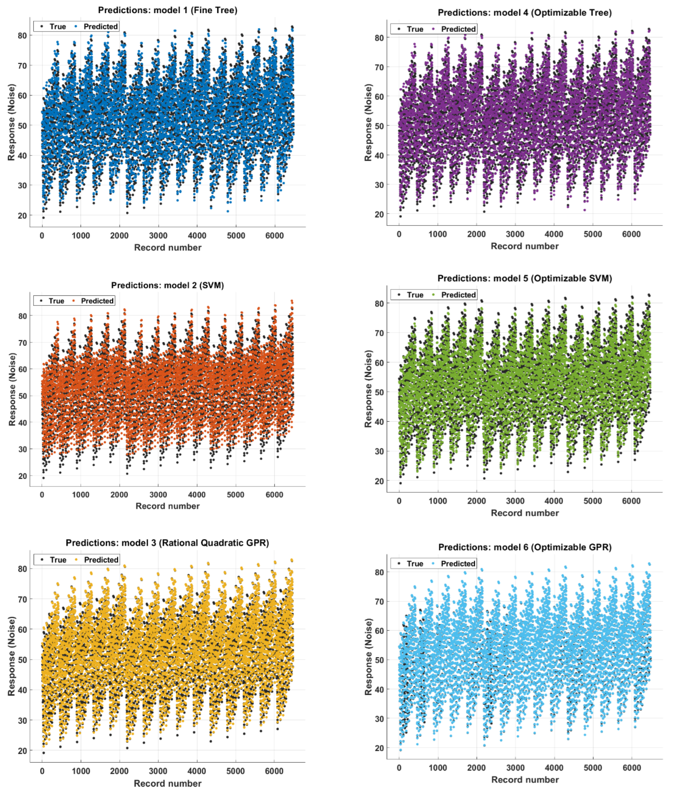
The noise prediction results of non-optimized and optimized regression models are additionally demonstrated through several of plots. The response plot (Figure 2) displays the predicted response for the validation observations and helps to assess the models’ ability to predict the noise pollution. As shown in Figure 2, the optimized GPR model (model 6) exhibited the highest level of accuracy, as evidenced by the close agreement between the predicted response values and the true values. Throughout the entire dataset, there was a significant overlap between the true and predicted samples, indicating the optimized GPR model’s high accuracy in predicting noise pollution.
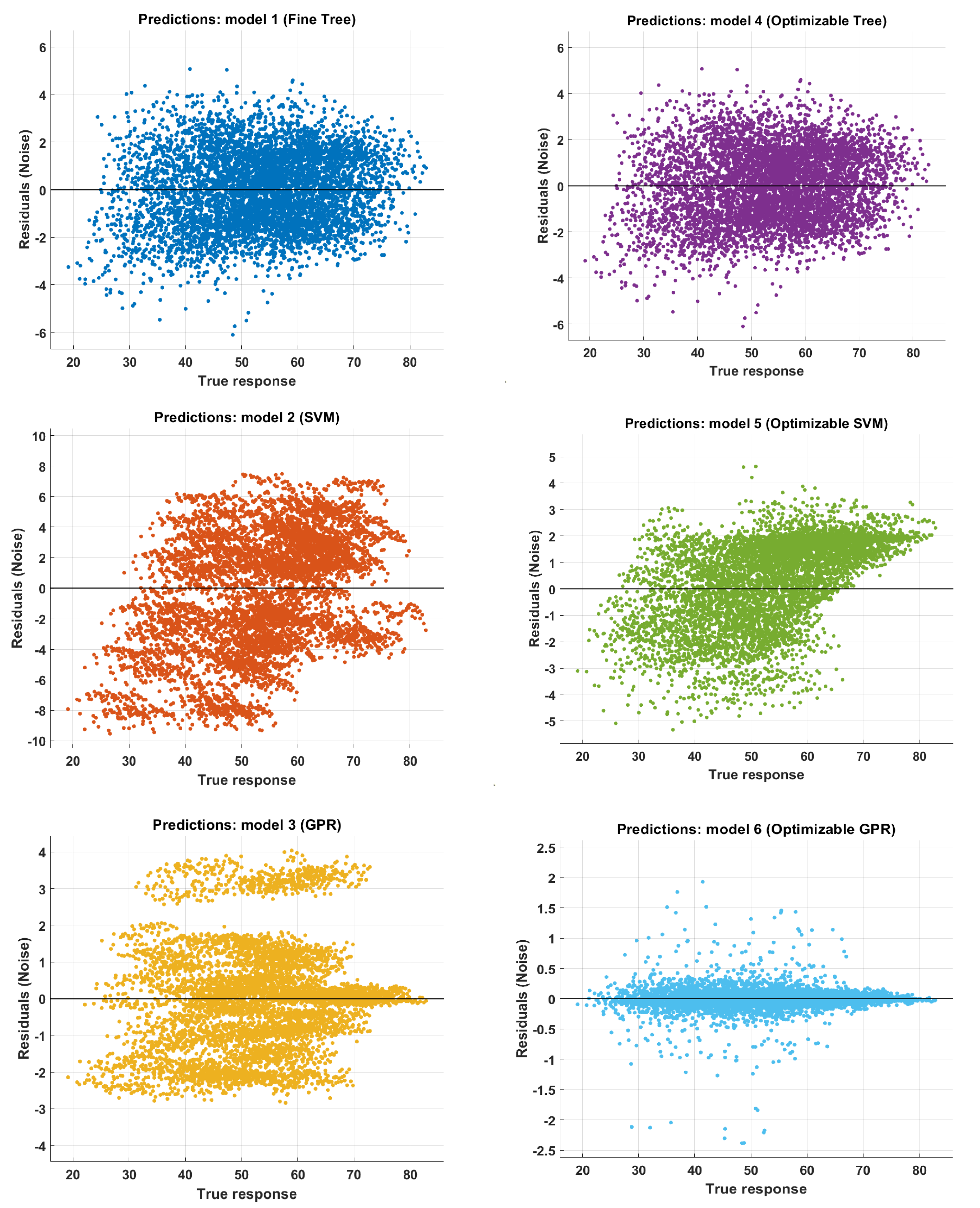
On the other hand, the residual plot (Figure 3) shows the difference between the estimated and actual responses, which is an important measure of the model’s performance. By observing the residuals, one can determine whether or not the model is making consistent predictions. As shown in Figure 3, the optimizable GPR (model 6) performed the best among all models, as indicated by the residuals being scattered symmetrically around 0. In contrast, the non-optimized SVM model (model 2) performed the worst, with residuals not displaying a clear pattern and their size changing significantly from left to right. The non-optimized fine tree model (model 1) and the optimized fine tree model (model 4) also displayed poor performance, with residuals not showing a clear pattern.
Lastly, the predicted versus actual response plot (Figure 4) compares the predicted response with the actual response and allows one to see how well the models fit the data. These plots provide a comprehensive evaluation of the model’s performances and are crucial in understanding the results of the study. As seen in Figure 4, the optimized GPR model (model 6) shows the best linear fit, with the points closely intersecting the diagonal line. This implies that the model has trained effectively, with the points scattered roughly symmetrically around the line. Other models, except model 2, also demonstrate good regression in predicting the noise variable.

4. Discussion of Major Findings

Given the results outlined in the preceding section, we can conclude the following:
  • Optimizing regression models improves noise-pollution prediction accuracy: In the study, optimization was performed on three regression models: regression trees, support vector machines, and Gaussian process regression. The objective was to determine the optimal values of hyper parameters for each model that would enhance their prediction performance. The optimization process significantly improved the accuracy of the noise-pollution predictions. This was confirmed by the improvement in performance measures such as MSE, RMSE, and R2. The optimization process allowed the models to better capture the underlying relationships between the predictors and the response, resulting in more accurate predictions of noise-pollution levels;
  • Optimized Gaussian process regression (GPR) model emerges as best performer: The results of the optimization process showed that the optimized GPR model emerged as the best performer among the three regression models. The optimized GPR model demonstrated the highest level of accuracy in terms of the performance measures, MSE, RMSE, and R2. It was able to effectively capture the relationships between the predictors and the response, resulting in highly accurate predictions of noise-pollution levels. The optimized GPR model outperformed the other models and emerged as the best model for predicting noise pollution. Despite being slower in terms of computation speed compared to the other models, its superior prediction accuracy makes it an ideal choice for use in addressing the problem of noise pollution;
  • The optimization of the Gaussian process regression (GPR) model was performed by determining the optimal values of the hyperparameters. The hyperparameters are parameters that control the shape of the regression function and, therefore, have a significant impact on the accuracy of the predictions. The optimization process involved searching for the optimal values of these parameters that would lead to the best performance of the model. The optimal values of the hyperparameters were found to be: a basis function of zero, a nonisotropic Matérn 3/2 kernel function, a kernel scale of 43.0096, and a sigma parameter of 0.42787. These values were crucial in ensuring the optimal performance of the GPR model for noise-pollution prediction. The GPR model with these hyperparameters delivered highly accurate predictions, outperforming other regression models. The optimization process improved the accuracy of the noise-pollution predictions and allowed for the creation of an effective solution for mitigating the impact of noise pollution in open area nearby main roads.
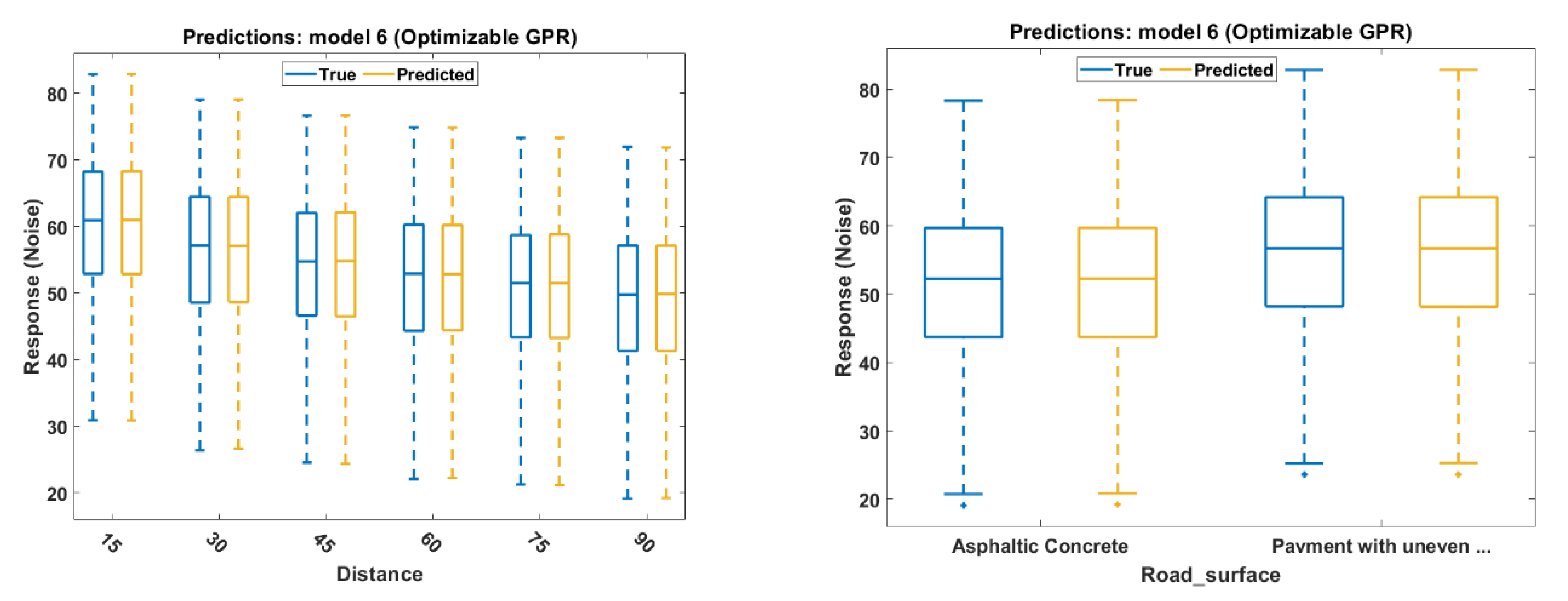
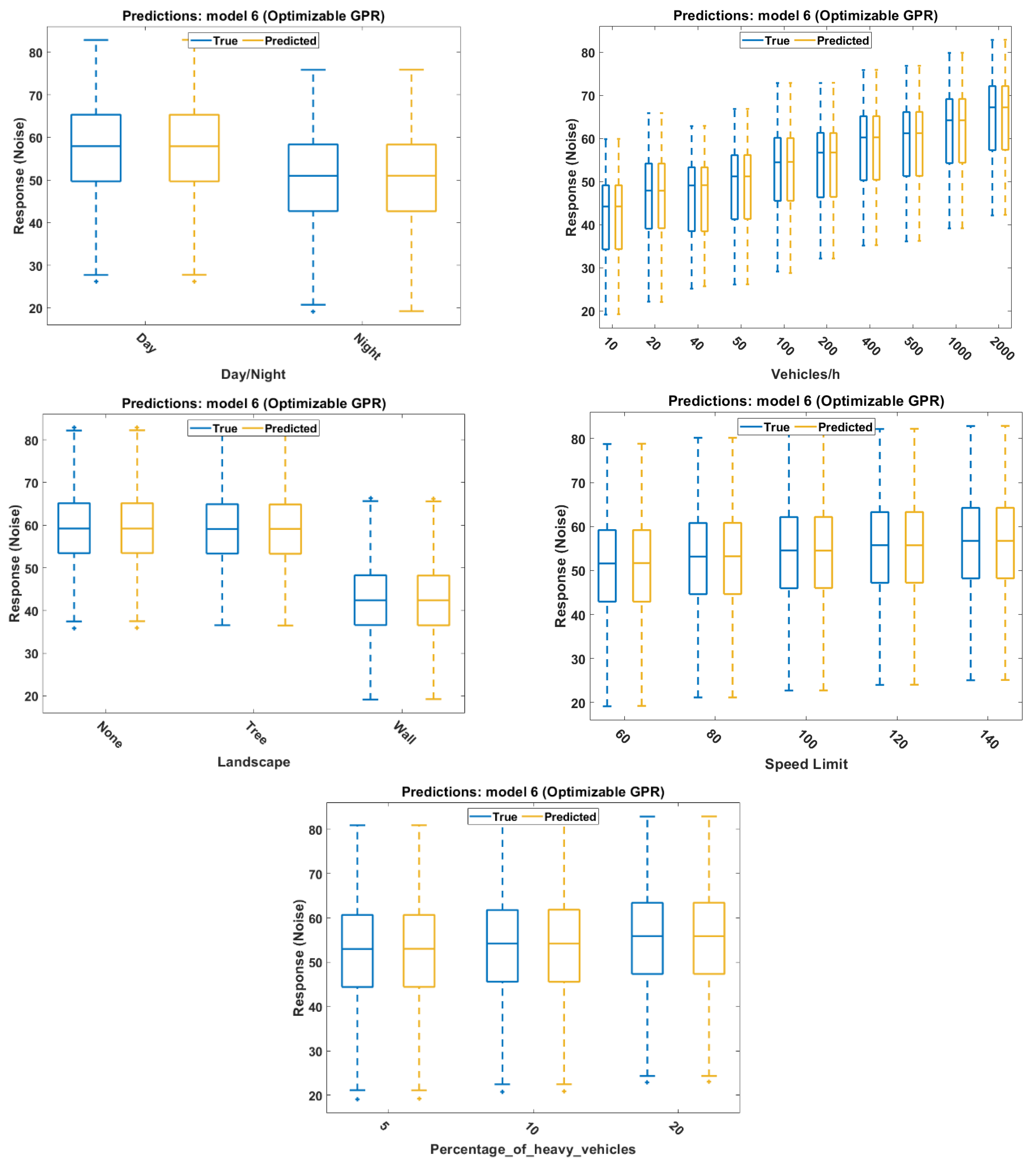
To further evaluate the effectiveness of the optimized Gaussian process regression (GPR) model, we presented box plots of the predictors and the response in Figure 5. The figure indicates that the model was able to achieve very accurate predictions of the noise variable for all given predictors. This suggests that the optimized GPR model is highly effective in predicting noise pollution and is capable of accurately capturing the relationship between the predictors and the response.
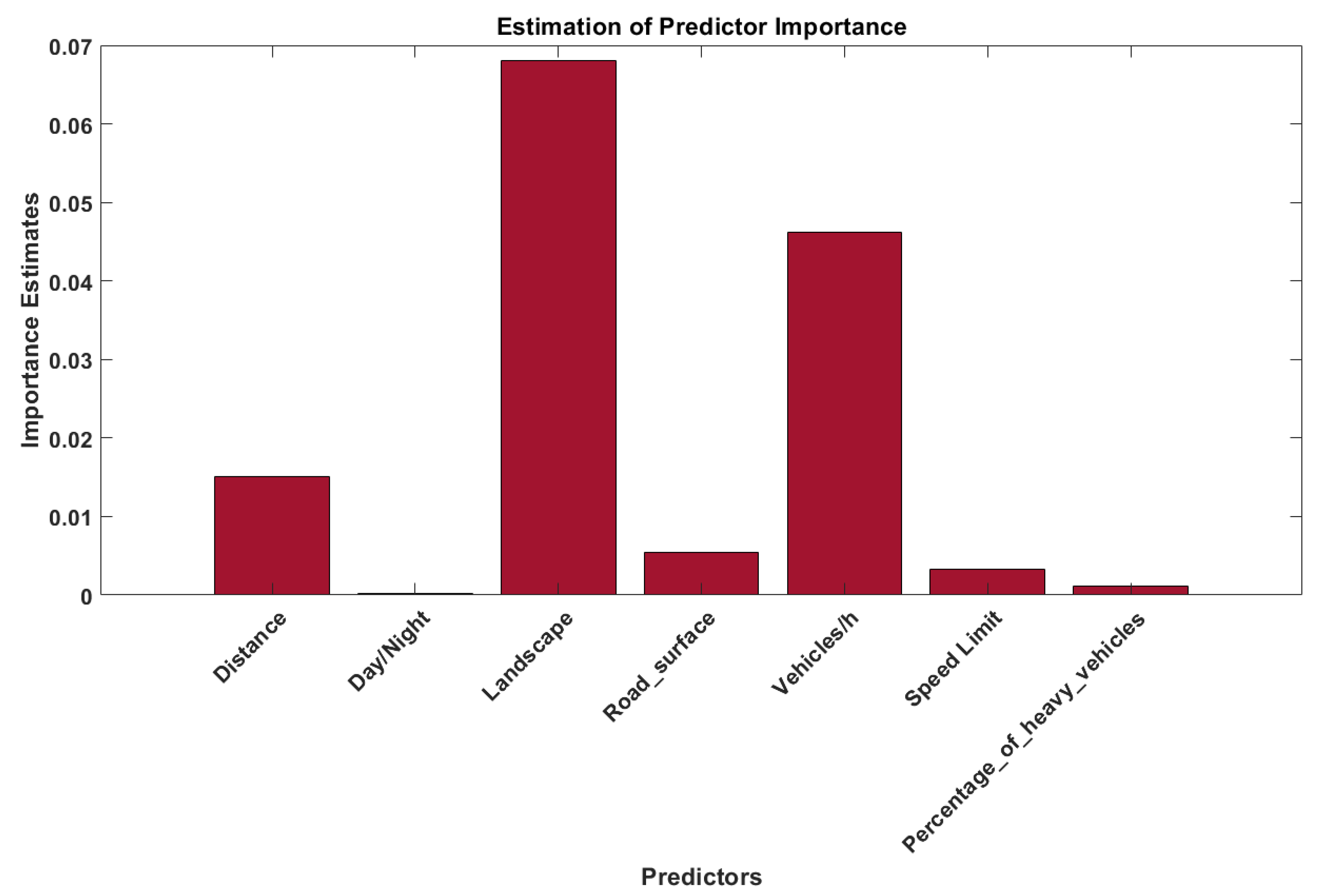
The features were further investigated using the best-performing model to assess their importance in predicting noise pollution. Figure 6 illustrates the results of predictor-importance analysis. The landscape emerges as the most influential predictor, followed closely by the number of vehicles per hour. The distance to the noise source also holds a certain level of significance. In contrast, the time of day, day and night classification, and the percentage of heavy vehicles are considered the least important predictors.
A final note on evaluating the best-performing model is that the performance of the best-performing model, the optimized Gaussian process regression (GPR), was compared to the results of previous studies. Table 5 provides a summary of the performance measures for the noise variables in these studies. To ensure a fair comparison, the prediction models used in these studies were also included. The results revealed that the model with the highest performance outperformed the state-of-the-art models in terms of the performance measures. The RMSE and MSE are metrics used to evaluate the performance of a regression model by quantifying the error rate. A lower value for these measures indicates a better model fit. In this case, the optimized GPR model outperforms the state-of-the-art models as evidenced by the RMSE value of 0.04 and MSE value of 0.19. These values indicate that the error-rate measures are at their lowest, further reinforcing the superiority of the proposed model over existing models.
On the other hand, the coefficient of determination (R2) represents the proportion of the dependent variable’s variation that can be predicted from the independent variable(s). The value of 1 signifies a perfect fit of the regression predictions to the data. The optimized GPR model achieves an R2 value of 1, which is the highest among the existing models. This further emphasizes the superiority of the model over the state-of-the-art models. This demonstrates the effectiveness of the optimized GPR model in predicting noise pollution, and highlights its superiority over the other models.

5. Conclusions

The increase in transportation activities has led to a rise in noise-pollution levels and safety concerns, particularly caused by traffic roads. To address this issue, this study aimed to estimate noise pollution caused by road traffic using various regression models (regression trees, support vector machines, and Gaussian process regression). To improve the accuracy of these models, the authors applied optimization techniques to the models and determined the optimal values of the hyperparameters using performance measures such as MSE, RMSE, and R2. The results showed that optimization significantly improved the performance of the models, with the optimized Gaussian process regression (GPR) model being the most accurate, delivering predictions with MSE of 0.19, RMSE of 0.04, and R2 of 1. Although the optimized GPR model was slower than the other models, it was still deemed the best performer due to its high accuracy. This study provides important insights into reducing noise pollution caused by road traffic and highlights the importance of hyperparameter optimization in improving prediction accuracy. The three key outcomes of the study were: (1) the optimization of regression models resulted in a significant improvement in noise-pollution prediction accuracy, (2) the optimized GPR model emerged as the best performer, delivering highly accurate predictions, and (3) the optimal values of the hyperparameters that were used to optimize the GPR model were found to be: a basis function of zero, a nonisotropic Matérn 3/2 kernel function, a kernel scale of 43.0096, and a sigma parameter of 0.42787, which were crucial in ensuring the optimal performance of the GPR model for noise-pollution prediction. These outcomes can serve as a guide for future experiments in the domain of noise pollution and similar fields.

Author Contributions

Conceptualization, A.A.A.-S., A.A., S.S.A. and U.B.; methodology, A.A.A.-S. and A.A.; software, A.A.A.-S. and A.A.; validation, U.B. and S.S.A.; formal analysis, A.A.A.-S., A.A. and A.A.M.A.; data curation, A.A.A.-S., A.A. and A.A.M.A.; writing—original draft preparation, A.A.A.-S. and A.A.; writing—review and editing, A.A.A.-S., A.A., S.S.A. and U.B.; visualization, A.A.A.-S. and A.A.; supervision, U.B. and S.S.A.; project administration, S.S.A. and A.A.; funding acquisition, S.S.A. All authors have read and agreed to the published version of the manuscript.

Funding

This research was funded by the Deanship of Scientific Research, Qassim University.

Data Availability Statement

The data presented in this study are available on request from the corresponding author. The data are not publicly available due to the rules of the local municipality.

Acknowledgments

The authors gratefully acknowledge Qassim University, represented by the Deanship of Scientific Research, on the financial support for this research under the number 10217-qec-2020-1-3-I during the academic year 1441 AH/2020 AD.

Conflicts of Interest

Authors declare that their work reported in this paper has not been influenced, or appeared to be influenced, by any competing financial interests or personal relationships.

Abbreviations

GPRGaussian process regression
MAEMean absolute error
MLMachine learning
MSEMean square error
R2R squared—coefficient of determination
RMSERoot means square error
SVMSupport vector machine

References

  1. Polson, N.G.; Sokolov, V.O. Deep learning for short-term traffic flow prediction. Transp. Res. Part C Emerg. Technol. 2017, 79, 1–17. [Google Scholar] [CrossRef] [Green Version]
  2. De Coensel, B.; Brown, A.L.; Tomerini, D. A road traffic noise pattern simulation model that includes distributions of vehicle sound power levels. Appl. Acoust. 2016, 111, 170–178. [Google Scholar] [CrossRef] [Green Version]
  3. Björkman, M. Community noise annoyance: Importance of noise levels and the number of noise events. J. Sound Vib. 1991, 151, 497–503. [Google Scholar] [CrossRef]
  4. Sato, T.; Yano, T.; Björkman, M.; Rylander, R. Road traffic noise annoyance in relation to average noise level, number of events and maximum noise level. J. Sound Vib. 1999, 223, 775–784. [Google Scholar] [CrossRef] [Green Version]
  5. Costa, L.G.; Cole, T.B.; Dao, K.; Chang, Y.C.; Coburn, J.; Garrick, J.M. Effects of air pollution on the nervous system and its possible role in neurodevelopmental and neurodegenerative disorders. Pharmacol. Ther. 2020, 210, 107523. [Google Scholar] [CrossRef]
  6. Sørensen, M.; Poulsen, A.H.; Hvidtfeldt, U.A.; Brandt, J.; Frohn, L.M.; Ketzel, M.; Christensen, J.H.; Im, U.; Khan, J.; Münzel, T.; et al. Air pollution, road traffic noise and lack of greenness and risk of type 2 diabetes: A multi-exposure prospective study covering Denmark. Environ. Int. 2022, 170, 107570. [Google Scholar] [CrossRef]
  7. Klompmaker, J.O.; Hoek, G.; Bloemsma, L.D.; Marra, M.; Wijga, A.H.; van den Brink, C.; Brunekreef, B.; Lebret, E.; Gehring, U.; Janssen, N.A. Surrounding green, air pollution, traffic noise exposure and non-accidental and cause-specific mortality. Environ. Int. 2020, 134, 105341. [Google Scholar] [CrossRef]
  8. WHO. Noise EURO; WHO: Geneva, Switzerland, 2019. [Google Scholar]
  9. Torija, A.J.; Ruiz, D.P. Automated classification of urban locations for environmental noise impact assessment on the basis of road-traffic content. Expert Syst. Appl. 2016, 53, 1–13. [Google Scholar] [CrossRef] [Green Version]
  10. Botteldooren, D.; Verkeyn, A.; Lercher, P. Noise Annoyance Modelling using Fuzzy Rule Based Systems. Noise Health 2002, 15, 27–44. [Google Scholar]
  11. Fallah-Shorshani, M.; Yin, X.; McConnell, R.; Fruin, S.; Franklin, M. Estimating traffic noise over a large urban area: An evalua-tion of methods. Environ. Int. 2022, 170, 107583. [Google Scholar] [CrossRef]
  12. Adulaimi, A.A.A.; Pradhan, B.; Chakraborty, S.; Alamri, A. Traffic Noise Modelling Using Land Use Regression Model Based on Machine Learning, Statistical Regression and GIS. Energies 2021, 14, 5095. [Google Scholar] [CrossRef]
  13. Yin, X.; Fallah-Shorshani, M.; McConnell, R.; Fruin, S.; Franklin, M. Predicting Fine Spatial Scale Traffic Noise Using Mobile Measurements and Machine Learning. Environ. Sci. Technol. 2020, 54, 12860–12869. [Google Scholar] [CrossRef]
  14. Nourani, V.; Gökçekuş, H.; Umar, I.K. Artificial intelligence based ensemble model for prediction of vehicular traffic noise. Environ. Res. 2020, 180, 108852. [Google Scholar] [CrossRef]
  15. Givargis, S.; Karimi, H. A basic neural traffic noise prediction model for Tehran’s roads. J. Environ. Manag. 2010, 91, 2529–2534. [Google Scholar] [CrossRef]
  16. Xu, D.; Wei, C.; Peng, P.; Xuan, Q.; Guo, H. GE-GAN: A novel deep learning framework for road traffic state estimation. Transp. Res. Part C Emerg. Technol. 2020, 117, 102635. [Google Scholar] [CrossRef]
  17. Can, A.; Chevallier, E.; Nadji, M.; Leclercq, L. Dynamic Traffic Modeling for Noise Impact Assessment of Traffic Strategies. Acta Acust. United Acust. 2010, 96, 482–493. [Google Scholar] [CrossRef]
  18. De Coensel, B.; De Muer, T.; Yperman, I.; Botteldooren, D. The influence of traffic flow dynamics on urban soundscapes. Appl. Acoust. 2005, 66, 175–194. [Google Scholar] [CrossRef] [Green Version]
  19. W Group. IMMI—Noise Prediction Software|Air Pollution Calculation Software. Available online: https://www.immi.eu/ (accessed on 7 January 2023).
  20. Gelbart, M.A.; Snoek, J.; Adams, R.P. Bayesian optimization with unknown constraints. arXiv 2014, arXiv:1403.5607. [Google Scholar]
  21. Vapnik, V.N. The Nature of Statistical Learning Theory; Springer: New York, NY, USA, 2000. [Google Scholar]
  22. Bravo-Moncayo, L.; Lucio-Naranjo, J.; Chávez, M.; Pavón-García, I.; Garzón, C. A machine learning approach for traffic-noise annoyance assessment. Appl. Acoust. 2019, 156, 262–270. [Google Scholar] [CrossRef]
  23. Chen, W.; An, J.; Li, R.; Fu, L.; Xie, G.; Bhuiyan, M.Z.A.; Li, K. A novel fuzzy deep-learning approach to traffic flow prediction with uncertain spatial–temporal data features. Futur. Gener. Comput. Syst. 2018, 89, 78–88. [Google Scholar] [CrossRef]
  24. Li, M.; Wang, Y.; Wang, Z.; Zheng, H. A deep learning method based on an attention mechanism for wireless network traffic prediction. Ad Hoc Netw. 2020, 107, 102258. [Google Scholar] [CrossRef]
  25. Lee, S.Y.; Le, T.H.M.; Kim, Y.M. Prediction and detection of potholes in urban roads: Machine learning and deep learning based image segmentation approaches. Dev. Built Environ. 2023, 13, 100109. [Google Scholar] [CrossRef]
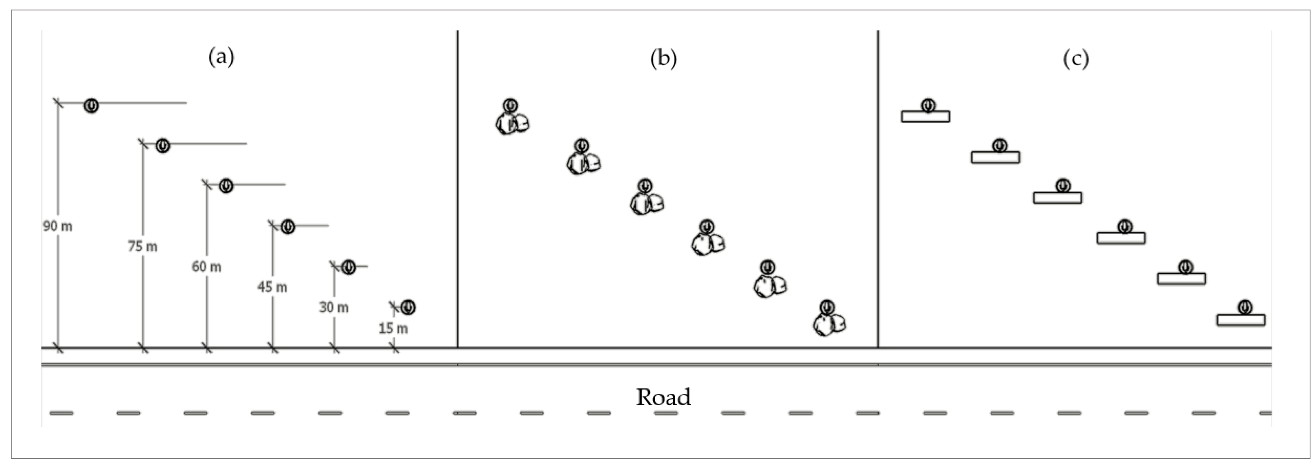
Figure 1. An illustration of the abstracted road layout and features values for the case study simulations: (a) receiver points without any barriers, (b) receiver points with trees (landscape), and (c) receiver points with walls (landscape).
Sustainability 15 10020 g001
Figure 2. Response plots of the non-optimized and optimized regression models.
Sustainability 15 10020 g002
Figure 3. Residuals’ plots of the non-optimized and optimized regression models.
Sustainability 15 10020 g003
Figure 4. Predicted vs. actual plots of the non-optimized and optimized regression models.
Sustainability 15 10020 g004
Figure 5. Box plots of the predictors vs. response (noise) based on the best-performed model (Model 6).
Sustainability 15 10020 g005aSustainability 15 10020 g005b
Figure 6. Importance of features in predicting noise pollution using the best-performing model.
Sustainability 15 10020 g006
Table 1. Features observed in this study.
FeaturesValuesNumber of
Observations
Target
Variable
Distance15, 30, 45, 60, 75, 90 (m)6480Noise
TimeDay, Night
LandscapeNone, Tree, Wall
Road surfaceAsphaltic concrete,
Uneven surface
Vehicles/h10, 20, 40, 50, 100, 200,
400, 500, 1000, 2000
Speed limit60, 80, 100, 120, 140 (km/h)
Percentage of
heavy vehicles
5, 10, 20 (%)
Table 2. The different hyperparameter options of the regression models.
Model TypeHyper-
Parameter
Without
Optimization
With Optimization
(Range of
Parameters’ Values)
Fine treeMinimum leaf size41–3240
SVMKernel functionLinearGaussian, Linear, Quadratic, Cubic
Kernel scaleAutomatic0.001–1000
Box constraintAutomatic0.001–1000
EpsilonAutomatic0.012042–1204.2254
Standardize dataTrueTrue, False
GPRBasis functionConstantConstant, Zero, Linear
Kernel functionRational QuadraticNonisotropic Rational Quadratic
Isotropic Rational Quadratic
Nonisotropic Squared Exponential
Isotropic Squared Exponential
Nonisotropic Matérn 5/2
Isotropic Matérn 5/2
Nonisotropic Matérn 3/2
Isotropic Matérn 3/2
Nonisotropic Exponential
Isotropic Exponential
Kernel scaleAutomatic1.99–1990
SigmaAutomatic0.0001–113.9076
StandardizeTrueTrue, False
Table 3. Prediction results of the regression models for noise pollution.
Model
Type
RMSER2MSEPrediction Speed
(obs/s) *
Training Time
SecMin
Non-optimizable
models
Model 1Fine tree1.590.982.52130,0003.150.05
Model 2SVM3.840.8914.7853,0007.190.12
Model 3GPR1.410.981.988100429.117.15
Optimizable modelsModel 4Fine tree1.570.982.48420,00021.200.35
Model 5SVM1.650.982.74260,0001206.6020.11
Model 6GPR0.191.000.0441008373.70139.56
* The prediction speed is measured by the number of observations processed per second.
Table 4. Best values of the hyperparameters for the regression models.
Model
Type
Hyper-
Parameter
With Optimization
RangeOptimal Value
Fine treeMinimum leaf size1–32403
SVMKernel functionGaussian, Linear, Quadratic, CubicGaussian
Kernel scale0.001–100078.5289
Box constraint0.001–1000588.2126
Epsilon0.012042–1204.22541.9145
Standardize dataTrue, FalseFalse
GPRBasis functionConstant, Zero, LinearZero
Kernel functionNonisotropic Rational QuadraticNonisotropic Matérn 3/2
Isotropic Rational Quadratic
Nonisotropic Squared Exponential
Isotropic Squared Exponential
Nonisotropic Matérn 5/2
Isotropic Matérn 5/2
Nonisotropic Matérn 3/2
Isotropic Matérn 3/2
Nonisotropic Exponential
Isotropic Exponential
Kernel scale1.99–199043.0096
Sigma0.0001–113.90760.42787
StandardizeTrue, FalseFalse
Table 5. The best-performing models in contrast to prior research.
ReferencePrediction
Model
MSERMSER2
[1]Deep-Learning Media Filter Preprocessing (DLM8L)7.7-0.85
[22]Artificial Neural Networks (ANN)-1.910.33
[11]eXtreme Gradient Boosting (XGB)0.65--
[23]Fuzzy Deep-Learning (FDCN)-0.30-
[24]Spatio-Temporal Convolutional Network
(LA-ResNet)
-4.5-
[25]Gaussian Process Regression (GPR)0.210.360.58
This studyOptimizable Gaussian Process Regression (GPR)—The best-performed model0.190.041.00
Disclaimer/Publisher’s Note: The statements, opinions and data contained in all publications are solely those of the individual author(s) and contributor(s) and not of MDPI and/or the editor(s). MDPI and/or the editor(s) disclaim responsibility for any injury to people or property resulting from any ideas, methods, instructions or products referred to in the content.