
Metabolic Process Modeling of Metal Resources Based on System Dynamics—A Case Study for Steel in Mainland China


Abstract
:1. Introduction
2. Materials and Methods
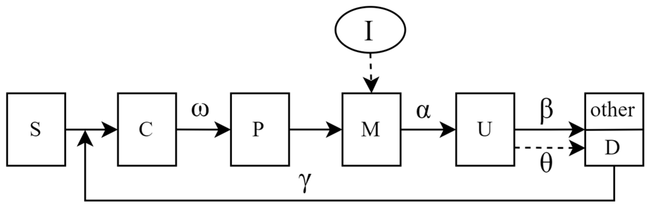
2.1. System Dynamics-Based Modeling of Steel Resource Metabolic Processes
2.2. Model Solving
2.2.1. Steel In-Use Stock U Solving
2.2.2. Model Parameter Solving
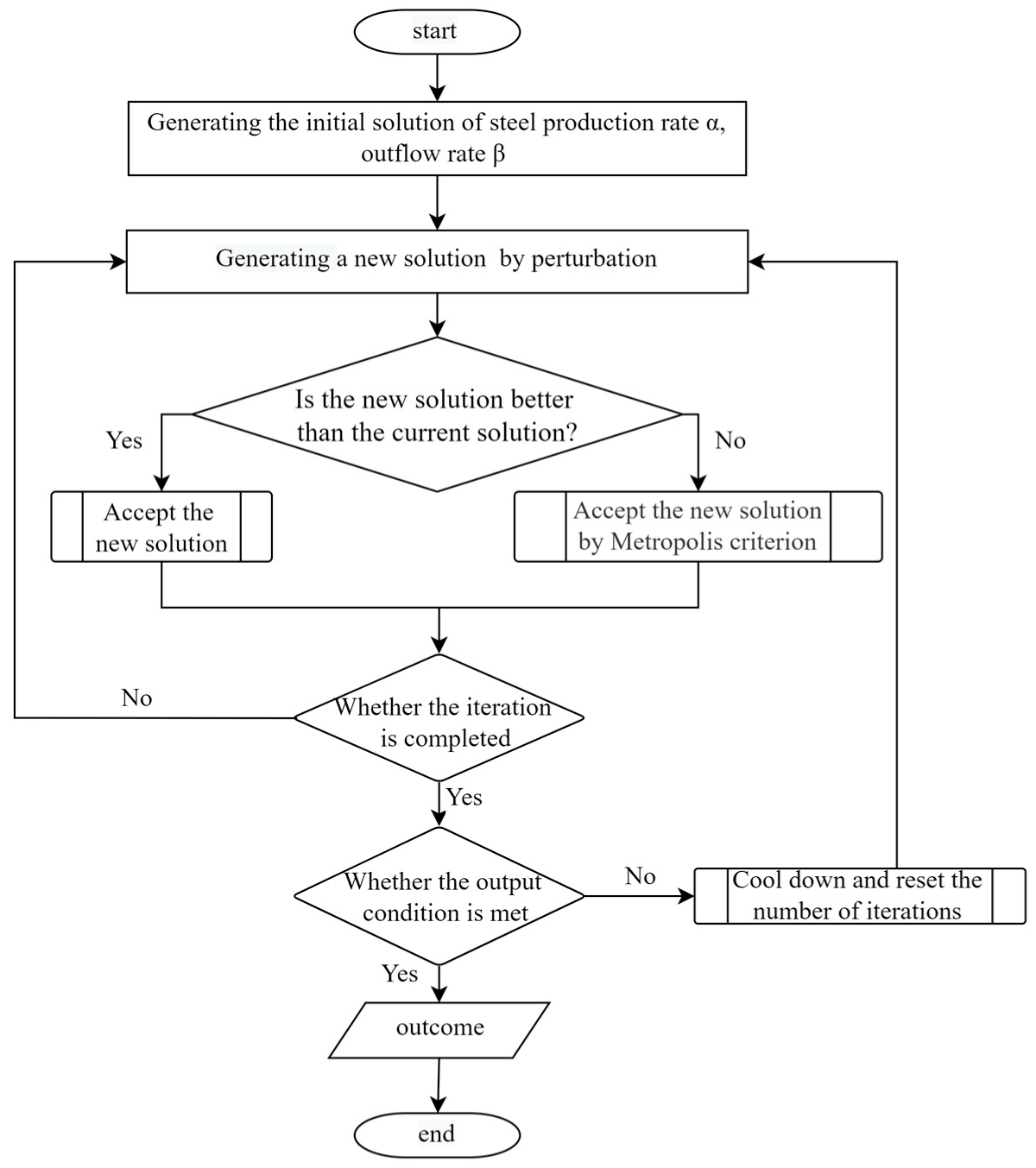
- (1)
- Select initial temperature T for the annealing solution, generate a random initial solution Xt for steel production rate α and outflow rate β, and then obtain the value of the objective function E(Xt) corresponding to the initial solution.
- (2)
- Set the rate of temperature decrease k, where k takes a value between 0 and 1.
- (3)
- Perturbation is implemented on the current solution to form a new solution Xt+1 for steel production rate α and outflow rate β, and the corresponding objective function value E(Xt+1) is then obtained and calculated:
- (4)
- If ΔE < 0, then accept the new solution as the current sister, otherwise judge whether to accept the new solution based on the Metropolis criterion.
- (5)
- Repeat the perturbation and acceptance process L times at temperature T, i.e., perform Steps 3 and 4.
- (6)
- Determine whether the temperature reaches the termination temperature level. If yes, the algorithm is terminated to obtain the final optimal solution. Otherwise, return to Step 2 to cool down and continue the perturbation solution.
3. System Boundary and Data Source
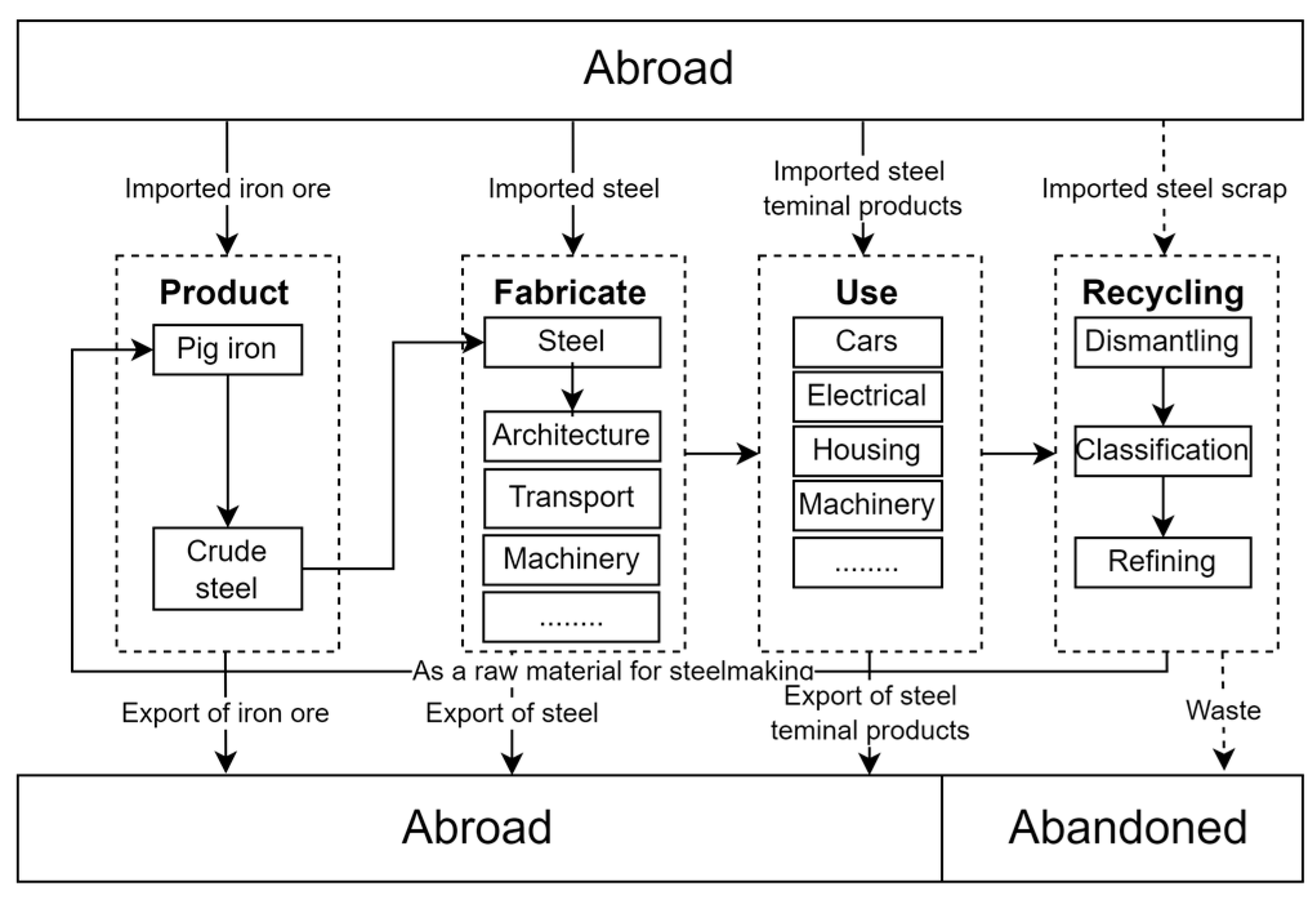
3.1. System Boundary
3.2. Data Sources and Presentation
4. Results
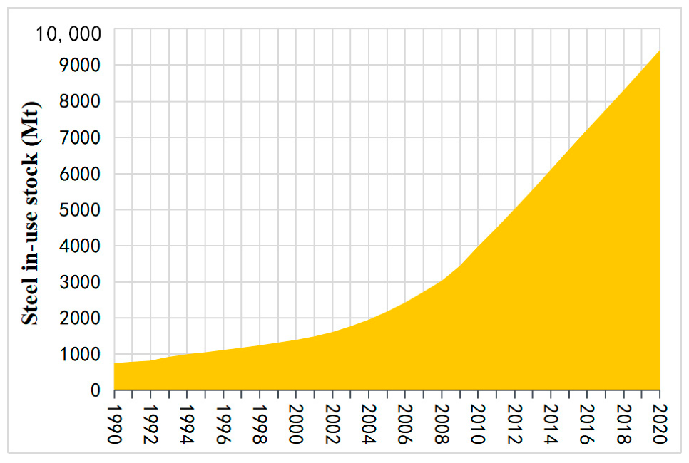
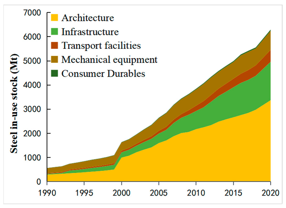
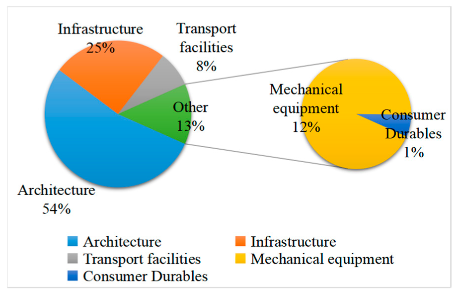
4.1. Analysis of Steel In-Use Stock Estimation Results
4.2. Solution Analysis of Steel Resource Metabolism Kinetic Model
4.2.1. National-Scale Steel Resource Metabolism Kinetic Model Solving
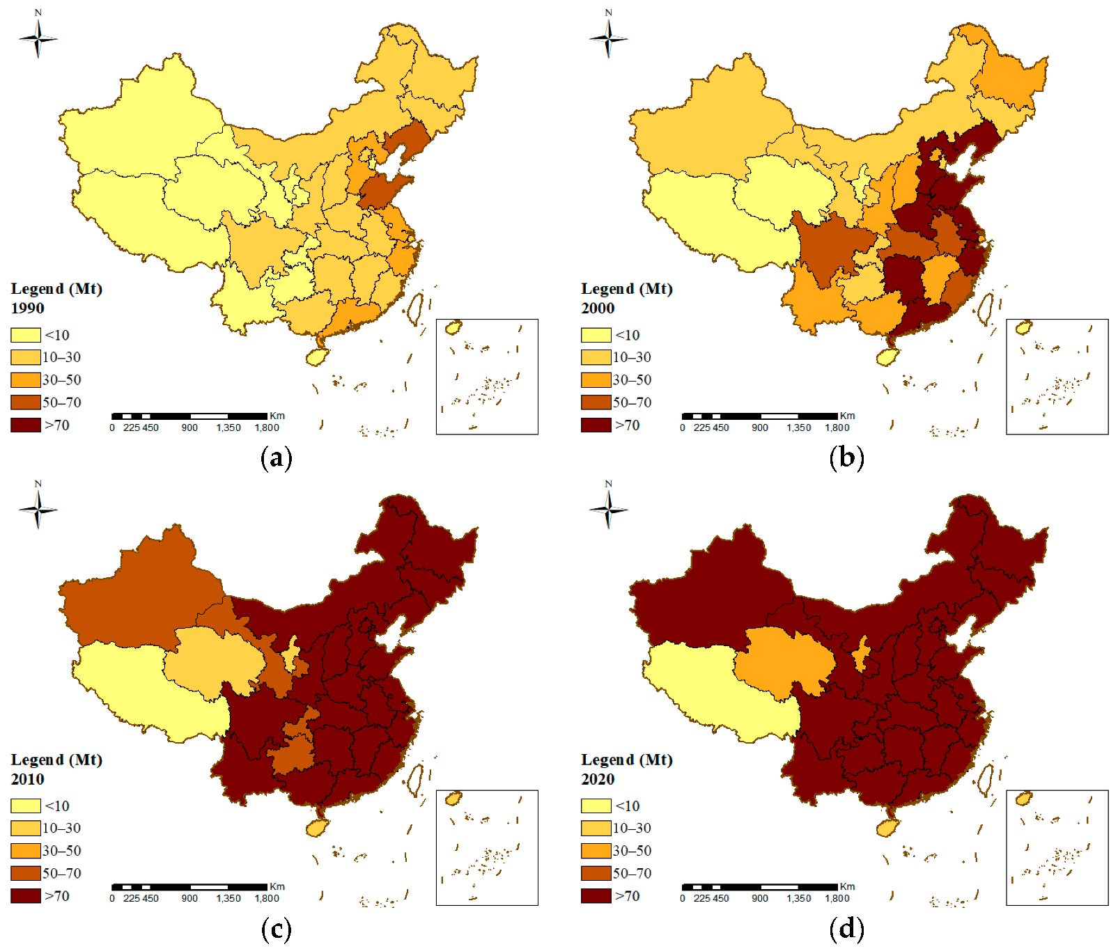
4.2.2. Kinetic Model Solving for the Provincial-Scale Metal Resource Metabolism
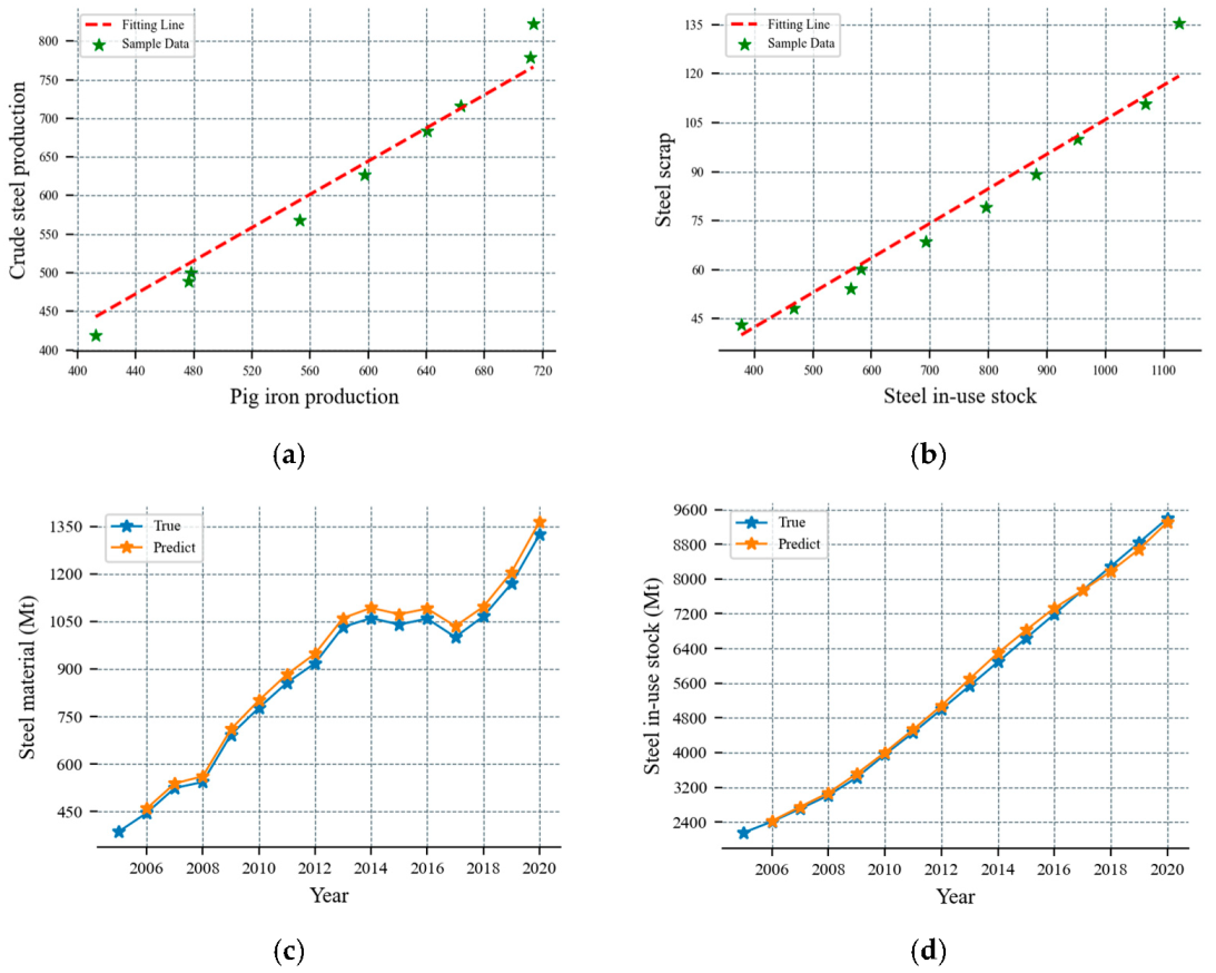
4.3. Steel Resource Metabolism Forecast
5. Discussion
5.1. Robustness and Limitations of Our Estimation
5.2. Policy Implications for Resource Sustainability
6. Conclusions
Author Contributions
Funding
Institutional Review Board Statement
Informed Consent Statement
Data Availability Statement
Conflicts of Interest
Appendix A

| Region | Year | Earlier Estimates | This Study | Difference |
|---|---|---|---|---|
| China | 2000 | 1.3 Gt [12] | 1.37 Gt | 5.4% |
| China | 2010 | 3.8 Gt [12] | 3.9 Gt | 2.6% |
| China | 2020 | 9.4 Gt [49] | 9.34 Gt | −0.64% |
| Tianjin | 2010 | 73 Mt [12] | 79.8 Mt | 9.3% |
| Hebei | 2010 | 219.5 Mt [12] | 154.7 Mt | −29.5% |
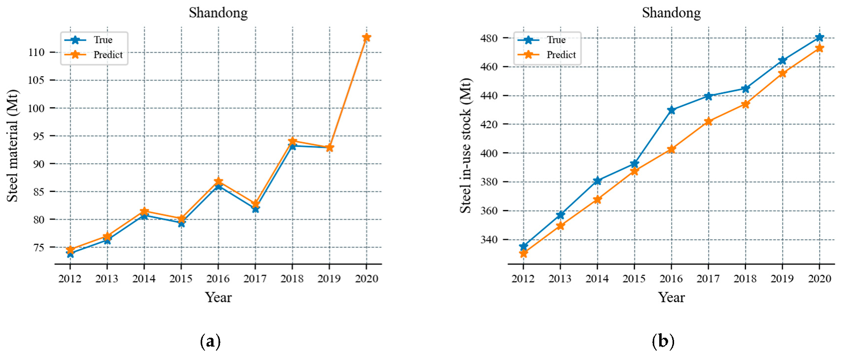
| Shandong | 2012 | 335.1 Mt [12] | 356.2Mt | 6.3% |
| Guangdong | 2012 | 391.5 Mt [12] | 439.1 Mt | 12.1% |
| Sichuan | 2010 | 149.4 Mt [12] | 174 Mt | 16.5% |
| Hunan | 2011 | 157.9 Mt [12] | 166.6 Mt | 5.5% |
| Hunan | 2019 | 215.4 Mt [12] | 244.8 Mt | 13.6% |
Appendix B
| Province | M Predict-M True R2 | U Predict-U True R2 | D Predict-D True R2 |
|---|---|---|---|
| Beijing | 0.773 | 0.864 | 0.807 |
| Tianjin | 0.983 | 0.489 | 0.808 |
| Hebei | 0.971 | 0.819 | 0.758 |
| Shanxi | 0.818 | 0.684 | 0.912 |
| Inner Mongolia | 0.945 | 0.952 | 0.820 |
| Liaoning | 0.919 | 0.613 | 0.900 |
| Jilin | 0.980 | 0.796 | 0.968 |
| Heilongjiang | 0.999 | 0.796 | 0.889 |
| Shanghai | 0.815 | 0.920 | 0.798 |
| Jiangsu | 0.935 | 0.871 | 0.653 |
| Zhejiang | 0.923 | 0.771 | 0.983 |
| Anhui | 0.845 | 0.920 | 0.728 |
| Fujian | 0.986 | 0.927 | 0.781 |
| Jiangxi | 0.911 | 0.922 | 0.934 |
| Shandong | 0.951 | 0.920 | 0.922 |
| Henan | 0.974 | 0.889 | 0.854 |
| Hubei | 0.696 | 0.872 | 0.799 |
| Hunan | 0.989 | 0.819 | 0.775 |
| Guangdong | 0.808 | 0.518 | 0.832 |
| Guangxi | 0.980 | 0.771 | 0.643 |
| Hainan | 0.906 | 0.689 | 0.643 |
| Chongqing | 0.992 | 0.919 | 0.724 |
| Sichuan | 0.977 | 0.931 | 0.996 |
| Guizhou | 0.898 | 0.787 | 0.503 |
| Yunnan | 0.918 | 0.927 | 0.852 |
| Shaanxi | 0.933 | 0.915 | 0.598 |
| Gansu | 0.857 | 0.892 | 0.604 |
| Qinghai | 0.292 | 0.335 | 0.968 |
| Ningxia | 0.783 | 0.938 | 0.833 |
| Xinjiang | 0.969 | 0.930 | 0.773 |
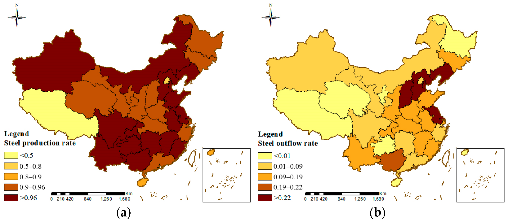
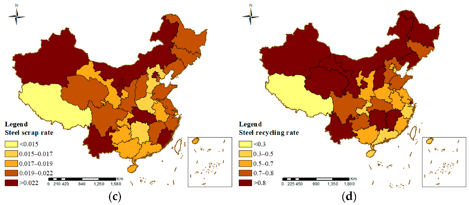
| Item | Steel Production Rate α | Steel Manufacturing Rate ω | Steel Outflow Rate β | Steel Scrap Rate θ | Steel Recycling Rate γ |
|---|---|---|---|---|---|
| China | 0.955 | 1.12 | 0.079 | 0.022 | 0.809 |
| Provincial average | 0.951 | 1.23 | 0.14 | 0.02 | 0.74 |
| Difference | −0.42% | 9.8% | 77.2% | −0.09% | −8.5% |
References
- The Raw-Materials Challenge: How the Metals and Mining Sector Will Be at the Core of Enabling the Energy Transition. Available online: https://www.mckinsey.com/industries/metals-and-mining/our-insights/the-raw-materials-challenge-how-the-metals-and-mining-sector-will-be-at-the-core-of-enabling-the-energy-transition (accessed on 5 November 2022).
- Recycling in Europe—Statistics & Facts. Available online: https://www.statista.com/topics/9617/recycling-in-europe/#topicOverview (accessed on 8 February 2023).
- Rieger, J.; Schenk, J. Residual Processing in the European Steel Industry: A Technological Overview. J. Sustain. Met. 2019, 5, 295–309. [Google Scholar] [CrossRef]
- Gulley, A.L.; Nassar, N.T.; Xun, S. China, the United States, and competition for resources that enable emerging technologies. Proc. Natl. Acad. Sci. USA 2018, 115, 4111–4115. [Google Scholar] [CrossRef] [PubMed] [Green Version]
- The Growing Importance of Steel Scrap in China. Available online: https://www.mckinsey.com/industries/metals-and-mining/our-insights/the-growing-importance-of-steel-scrap-in-china (accessed on 1 March 2017).
- Ayres, R.U. The Greening of Industrial Ecosystems. In Industrial Metabolism: Theory and Policy; National Academy Press: Washington, DC, USA, 1994; pp. 23–37. [Google Scholar]
- Sun, Q.; Li, H.; Xu, B.; Cheng, L.; Wennersten, R. Analysis of secondary energy in China’s iron and steel industry—An approach of industrial metabolism. Int. J. Green Energy 2016, 13, 793–802. [Google Scholar] [CrossRef]
- Zhang, L.; Yuan, Z.W.; Bi, J. Substance flow analysis (SFA): A critical review. Acta Ecol. Sin. 2009, 29, 6189–6198. [Google Scholar]
- Dai, T.J. A study on material metabolism in Hebei iron and steel industry analysis. Resour. Conserv. Recycl. 2015, 95, 183–192. [Google Scholar] [CrossRef]
- Guo, Z.; Hu, D.; Zhang, F.; Huang, G.; Xiao, Q. An integrated material metabolism model for stocks of urban road system in Beijing, China. Sci. Total. Environ. 2014, 470, 883–894. [Google Scholar] [CrossRef]
- Liu, Y.; Li, J.; Chen, W.; Song, L.; Dai, S. Quantifying urban mass gain and loss by a GIS-based material stocks and flows analysis. J. Ind. Ecol. 2022, 26, 1051–1060. [Google Scholar] [CrossRef]
- Song, L.; Han, J.; Li, N.; Huang, Y.; Hao, M.; Dai, M.; Chen, W.-Q. China material stocks and flows account for 1978–2018. Sci. Data 2021, 8, 303. [Google Scholar] [CrossRef]
- Li, Q.; Gao, T.; Wang, G.; Cheng, J.; Dai, T.; Wang, H. Dynamic analysis of iron flows and in-use stocks in China: 1949–2015. Resour. Policy 2018, 62, 625–634. [Google Scholar] [CrossRef]
- Song, L.; Zhang, C.; Han, J.; Chen, W.-Q. In-use product and steel stocks sustaining the urbanization of Xiamen, China. Ecosyst. Health Sustain. 2019, 5, 110–123. [Google Scholar] [CrossRef] [Green Version]
- Hao, M.; Wang, P.; Song, L.; Dai, M.; Ren, Y.; Chen, W.-Q. Spatial distribution of copper in-use stocks and flows in China: 1978–2016. J. Clean. Prod. 2020, 261, 121260. [Google Scholar] [CrossRef]
- Duan, L.; Liu, Y.; Yang, Y.; Song, L.; Hao, M.; Li, J.; Dai, M.; Chen, W.-Q. Spatiotemporal dynamics of in-use copper stocks in the Jing-Jin-Ji urban agglomeration, China. Resour. Conserv. Recycl. 2021, 175, 105848. [Google Scholar] [CrossRef]
- Chen, W.-Q.; Graedel, T. Dynamic analysis of aluminum stocks and flows in the United States: 1900–2009. Ecol. Econ. 2012, 81, 92–102. [Google Scholar] [CrossRef]
- Recalde, K.; Wang, J.; Graedel, T. Aluminium in-use stocks in the state of Connecticut. Resour. Conserv. Recycl. 2008, 52, 1271–1282. [Google Scholar] [CrossRef]
- Augiseau, V.; Barles, S. Studying construction materials flows and stock: A review. Resour. Conserv. Recycl. 2017, 123, 153–164. [Google Scholar] [CrossRef]
- Pauliuk, S.; Wang, T.; Müller, D.B. Moving Toward the Circular Economy: The Role of Stocks in the Chinese Steel Cycle. Environ. Sci. Technol. 2011, 46, 148–154. [Google Scholar] [CrossRef] [Green Version]
- Wang, P.; Li, W.; Kara, S. Cradle-to-cradle modeling of the future steel flow in China. Resour. Conserv. Recycl. 2017, 117, 45–57. [Google Scholar] [CrossRef]
- Han, J.; Xiang, W.-N. Analysis of material stock accumulation in China’s infrastructure and its regional disparity. Sustain. Sci. 2012, 8, 553–564. [Google Scholar] [CrossRef]
- Liu, Q.; Cao, Z.; Liu, X.; Liu, L.; Dai, T.; Han, J.; Liu, G. Product and metal stocks accumulation of China’s megacities: Patterns, drivers, and implications. Environ. Sci. Technol. 2019, 53, 4128–4139. [Google Scholar] [CrossRef] [Green Version]
- Parajuly, K.; Habib, K.; Liu, G. Waste electrical and electronic equipment (WEEE) in Denmark: Flows, quantities and management. Resour. Conserv. Recycl. 2017, 123, 85–92. [Google Scholar] [CrossRef]
- Zhang, L.; Xie, M.; Tang, L. Bias correction for the least squares estimator of Weibull shape parameter with complete and censored data. Reliab. Eng. Syst. Saf. 2006, 91, 930–939. [Google Scholar] [CrossRef]
- Zhao, F.; Yue, Q.; He, J.; Li, Y.; Wang, H. Quantifying China’s iron in-use stock and its driving factors analysis. J. Environ. Manag. 2020, 274, 111220. [Google Scholar] [CrossRef]
- Song, L.; Dai, S.; Cao, Z.; Liu, Y.; Chen, W.-Q. High spatial resolution mapping of steel resources accumulated above ground in mainland China: Past trends and future prospects. J. Clean. Prod. 2021, 297, 126482. [Google Scholar] [CrossRef]
- Zhang, Y.; Zhao, H.; Yu, Y.; Wang, T.; Zhou, W.; Jiang, J.; Chen, D.; Zhu, B. Copper in-use stocks accounting at the sub-national level in China. Resour. Conserv. Recycl. 2019, 147, 49–60. [Google Scholar] [CrossRef]
- Forrester, J.W. Industrial dynamics: A major breakthrough for decision makers. Harv. Bus. Rev. 1958, 36, 37–66. [Google Scholar]
- Forrester, J.W. Principles of Systems; Wright-Allen Press: Cambridge, MA, USA, 1968. [Google Scholar]
- Forrester, J.W. Industrial dynamics. J. Oper. Res. Soc. 1997, 48, 1037–1041. [Google Scholar] [CrossRef]
- Liu, Y. A system dynamics approach for corporate waste recycling capacity and income. In Proceedings of the 2010 International Conference on E-Business and E-Government, Guangzhou, China, 7–9 May 2010; pp. 3615–3618. [Google Scholar]
- Dyson, B.; Chang, N.-B. Forecasting municipal solid waste generation in a fast-growing urban region with system dynamics modeling. Waste Manag. 2005, 25, 669–679. [Google Scholar] [CrossRef]
- Chaerul, M.; Tanaka, M.; Shekdar, A.V. A system dynamics approach for hospital waste management. Waste Manag. 2008, 28, 442–449. [Google Scholar] [CrossRef]
- Ullibeer, S. Dynamic interactions between citizen choice and preferences and public policy initiatives: A system dynamics model of recycling dynamics in a typical Swiss locality. In Proceedings of the 21st International Conference of the System Dynamics Society, New York, NY, USA, 20–24 July 2003. [Google Scholar]
- House, T.S. Law of conservation of mass. chemical education. Chem. Educ. 1967, 15, 34–37. [Google Scholar]
- Metropolis, N.; Rosenbluth, A.W.; Rosenbluth, M.N.; Teller, A.H.; Teller, E. Equation of State Calculations by Fast Computing Machines. J. Chem. Phys. 1953, 21, 1087–1092. [Google Scholar] [CrossRef] [Green Version]
- Theil, H.; Cramer, J.S.; Moerman, H.; Russchen, A. Economic Forecasts and Policy, 2nd ed.; North-Holland Publishing Company: Amsterdam, The Netherlands, 1970. [Google Scholar]
- Geospatial Data Cloud Site, Computer Network Information Center, Chinese Academy of Sciences. 2018. Available online: http://www.gscloud.cn/ (accessed on 19 January 2013).
- National Bureau of Statistics. China Statistical Yearbook 1991–2021; China Statistic Press: Beijing, China, 2021.
- Hunan Provincial Bureau of Statistics. Hunan Statistical Yearbook 1991–2021; China Statistic Press: Beijing, China, 2021.
- Editorial Board of China Steel Yearbook. China Steel Yearbook 1991–2021; China Steel Yearbook Press: Beijing, China, 2021. [Google Scholar]
- Wang, T.; Müller, D.B.; Hashimoto, S. The Ferrous Find: Counting Iron and Steel Stocks in China’s Economy. J. Ind. Ecol. 2015, 19, 877–889. [Google Scholar] [CrossRef]
- YB/T 177-2000; Metallurgical Industry Bureau of China. Standards for Continuous Casting Ductile Iron Pipes. China Standard Press: Beijing, China, 2000.
- China Iron and Steel Industry Association. China Steel Industry Statistics Compendium, 1949–2000; Metallurgical Industry Press: Beijing, China, 2003.
- Steel Scrap to Crude Steel Ratio in Steel Production in China from 2014 to 2021. Available online: https://www.statista.com/statistics/1071833/china-steel-scrap-recycling-rate/ (accessed on 23 March 2023).
- Gordon, R.B.; Bertram, M.; Graedel, T.E. From the cover: Metal stocks and sustainability. Proc. Natl. Acad. Sci. USA 2006, 103, 1209–1214. [Google Scholar] [CrossRef] [PubMed] [Green Version]
- Gerst, M.D.; Graedel, T.E. In-Use Stocks of Metals: Status and Implications. Environ. Sci. Technol. 2008, 42, 7038–7045. [Google Scholar] [CrossRef] [PubMed]
- List of Steel Accumulation per Capita in China. Available online: https://blog.sina.com.cn/s/blog_50321d940101vatv.html (accessed on 12 April 2014).


| Description | Steel Production Rate α | Steel Manufacturing Rate ω | Steel Outflow Rate β | Steel Scrap Rate θ | Steel Recycling Rate γ |
|---|---|---|---|---|---|
| Solution of the value | 0.955 | 1.12 | 0.079 | 0.022 | 0.809 |
| R2 | 0.95 | 0.665 | 0.96 | 0.756 | 0.81 |
| Province | Steel Production Rate α | Steel Manufacturing Rate ω | Steel Outflow Rate β | Steel Scrap Rate θ | Steel Recycling Rate γ | Loss |
|---|---|---|---|---|---|---|
| Beijing | 0.76217 | 1.3843 | 0.015 | 0.02388 | 0.69265 | 0.009 |
| Tianjin | 0.96004 | 2.6887 | 0.60916 | 0.02071 | 0.44051 | 0.05 |
| Hebei | 0.99247 | 1.2184 | 0.80102 | 0.01665 | 0.78521 | 0.01 |
| Shanxi | 0.95075 | 0.9936 | 0.27596 | 0.02157 | 0.93014 | 0.03 |
| Inner Mongolia | 0.97968 | 0.9914 | 0.06684 | 0.02292 | 0.93534 | 0.01 |
| Liaoning | 0.97221 | 1.0583 | 0.27376 | 0.02089 | 0.99232 | 0.01 |
| Jilin | 0.95820 | 1.1153 | 0.15747 | 0.02030 | 0.76493 | 0.02 |
| Heilongjiang | 0.93069 | 0.8892 | 0.00850 | 0.02164 | 0.96935 | 0.01 |
| Shanghai | 0.94702 | 1.1538 | 0.10713 | 0.01554 | 0.96555 | 0.006 |
| Jiangsu | 0.98409 | 1.3260 | 0.23475 | 0.02019 | 0.66627 | 0.01 |
| Zhejiang | 0.93343 | 2.5243 | 0.07094 | 0.02032 | 0.39380 | 0.02 |
| Anhui | 0.96783 | 1.2384 | 0.11391 | 0.01797 | 0.68887 | 0.004 |
| Fujian | 0.97479 | 1.6209 | 0.12355 | 0.02471 | 0.68829 | 0.012 |
| Jiangxi | 0.97711 | 1.1039 | 0.17170 | 0.02095 | 0.84622 | 0.007 |
| Shandong | 0.98358 | 1.2904 | 0.16221 | 0.02077 | 0.78528 | 0.008 |
| Henan | 0.95826 | 1.4394 | 0.12406 | 0.01646 | 0.66669 | 0.009 |
| Hubei | 0.95787 | 1.1792 | 0.10971 | 0.02393 | 0.72683 | 0.02 |
| Hunan | 0.97931 | 1.0581 | 0.05327 | 0.01521 | 0.98861 | 0.02 |
| Guangdong | 0.93608 | 1.8789 | 0.06703 | 0.01861 | 0.35664 | 0.01 |
| Guangxi | 0.98009 | 1.5430 | 0.19023 | 0.01811 | 0.69393 | 0.03 |
| Hainan | 0.84607 | 0.0003 | 0.00030 | 0.01702 | 0.47892 | 0.12 |
| Chongqing | 0.96486 | 1.8376 | 0.09733 | 0.01780 | 0.47678 | 0.004 |
| Sichuan | 0.98493 | 1.3101 | 0.05964 | 0.01902 | 0.72196 | 0.02 |
| Guizhou | 0.97393 | 1.0295 | 0.00106 | 0.01856 | 0.78082 | 0.04 |
| Yunnan | 0.96640 | 1.0641 | 0.10823 | 0.02256 | 0.96446 | 0.01 |
| Shaanxi | 0.95688 | 1.4774 | 0.09364 | 0.01914 | 0.58563 | 0.01 |
| Gansu | 0.90719 | 1.0503 | 0.05460 | 0.01862 | 0.82213 | 0.01 |
| Qinghai | 0.95249 | 0.9777 | 0.00038 | 0.01971 | 0.96967 | 0.09 |
| Ningxia | 0.94025 | 1.0743 | 0.00075 | 0.02218 | 0.50731 | 0.04 |
| Xinjiang | 0.96346 | 1.1783 | 0.08511 | 0.02459 | 0.82474 | 0.01 |
Disclaimer/Publisher’s Note: The statements, opinions and data contained in all publications are solely those of the individual author(s) and contributor(s) and not of MDPI and/or the editor(s). MDPI and/or the editor(s) disclaim responsibility for any injury to people or property resulting from any ideas, methods, instructions or products referred to in the content. |
© 2023 by the authors. Licensee MDPI, Basel, Switzerland. This article is an open access article distributed under the terms and conditions of the Creative Commons Attribution (CC BY) license (https://creativecommons.org/licenses/by/4.0/).
Share and Cite
Shi, Y.; Shao, S.; Yang, X.; Wang, D.; Chen, B.; Deng, M. Metabolic Process Modeling of Metal Resources Based on System Dynamics—A Case Study for Steel in Mainland China. Sustainability 2023, 15, 10249. https://doi.org/10.3390/su151310249
Shi Y, Shao S, Yang X, Wang D, Chen B, Deng M. Metabolic Process Modeling of Metal Resources Based on System Dynamics—A Case Study for Steel in Mainland China. Sustainability. 2023; 15(13):10249. https://doi.org/10.3390/su151310249
Chicago/Turabian StyleShi, Yan, Shanshan Shao, Xuexi Yang, Da Wang, Bingrong Chen, and Min Deng. 2023. "Metabolic Process Modeling of Metal Resources Based on System Dynamics—A Case Study for Steel in Mainland China" Sustainability 15, no. 13: 10249. https://doi.org/10.3390/su151310249