Enhancing Forest Canopy Height Retrieval: Insights from Integrated GEDI and Landsat Data Analysis

Abstract

Canopy height is a crucial indicator for assessing the structure and function of the forest ecosystems. It plays a significant role in carbon sequestration, sink enhancement, and promoting green development. This study aimed to evaluate the accuracy of GEDI L2A version 2 data in estimating ground elevation and canopy height by comparing it with airborne laser scanning (ALS) data. Among the six algorithms provided by the GEDI L2A data, algorithm a2 demonstrated higher accuracy than the others in detecting ground elevation and canopy height. Additionally, a relatively strong correlation (R-squared = 0.35) was observed between rh95 for GEDI L2A and RH90 for ALS. To enhance the accuracy of canopy height estimation, this study proposed three backpropagation (BP) neural network inversion models based on GEDI, Landsat 8 OLI, and Landsat 9 OLI-2 data. Multiple sets of relative heights and vegetation indices were extracted from the GEDI and Landsat datasets. The random forest (RF) algorithm was employed to select feature variables with a cumulative importance score of 90% for training the BP neural network inversion models. Validation against RH90 of ALS revealed that the GEDI model outperformed the OLI or OLI-2 data models in terms of accuracy. Moreover, the quality improvement of OLI-2 data relative to OLI data contributed to enhanced inversion accuracy. Overall, the models based on a single dataset exhibited relatively low accuracy. Hence, this study proposed the GEDI and OLI and GEDI and OLI-2 models, which combine the two types of data. The results demonstrated that the combined model integrating GEDI and OLI-2 data exhibited the highest performance. Compared to the weakest OLI data model, the inversion accuracy R-squared improved from 0.38 to 0.74, and the MAE, RMSE, and rRMSE decreased by 1.21 m, 1.81 m, and 8.09%, respectively. These findings offer valuable insights for the remote sensing monitoring of forest sustainability.

1. Introduction

Forest canopy height, which can reflect the productivity level of forest ecosystems in vertical structures, is an important attribute for forest biomass estimation, forest management, and assessment of habitat quality [1,2,3]. Forest biomass research plays a crucial role in the global carbon cycle, and is of great significance for understanding the response of forest ecosystems to global climate change, as well as for formulating carbon emission policies and mitigating global warming [4,5].

Remote-sensing technology can accurately and rapidly obtain continuous forest information [6]. Data commonly used for estimating forest canopy height can be classified into optical, microwave, and lidar data [7,8,9]. Common optical sensors include remote sensing instruments on satellites (such as OLI and MODIS) and cameras mounted on unmanned aerial vehicles (UAVs) [10,11]. Optical sensors measure the radiation energy in the visible and near-infrared bands to gather surface information. By analyzing the spectral characteristics and spatial patterns of vegetation, previous studies have successfully estimated forest height using optical remote sensing [12,13,14,15]. However, it is important to note that optical sensors are limited by factors such as cloud cover and daylight conditions, which make them unsuitable for cloud-dense or nighttime observations [16]. Microwave sensors, on the other hand, can penetrate through cloud cover and forest canopies, allowing them to retrieve information from the underlying surface [17]. Radar satellites like RADARSAT and Sentinel-1, as well as synthetic aperture radar (SAR), are examples of microwave sensors commonly used for forest canopy height inversion [18,19]. These sensors estimate canopy height by measuring the backscattering intensity and phase of microwave signals. Microwave signals exhibit strong penetration capabilities for vegetation biomass estimation, but they generally have lower spatial resolution, making it challenging to provide detailed information about the structure of vegetation [20]. Lidar sensors employ laser beams to emit pulses of light and measure the time it takes for the signals to return after interacting with objects on the Earth’s surface [21]. This technology enables accurate height measurements of surface objects, including the forest canopy [22]. Lidar systems, such as ALS and ground-based laser scanning, possess high vertical resolution, making them particularly suitable for mapping canopy height [23,24]. However, it is worth noting that lidar systems typically have lower horizontal resolution compared to optical and microwave sensors [25]. Moreover, lidar measurements can be influenced by factors such as ground cover and the density of the forest canopy [26].

A variety of data has led to diverse methods for mapping forest canopy height, which can be grouped into parametric algorithms, physical models, and machine-learning algorithms [19,27,28,29,30]. Parametric algorithms utilize mathematical models to establish relationships between optical, microwave, or lidar data and ground measurements in order to estimate canopy height [27,31]. These algorithms often rely on manually selected features and indices, such as vegetation indices and backscatter intensity. While parametric algorithms are user-friendly and straightforward, they may lack accuracy when dealing with complex terrains and vegetation structures. In contrast, physical models leverage the principles of optical, microwave, or lidar radiation transfer processes [32]. By simulating the interactions of light or beams within vegetation, these models infer canopy height. Physical models provide a deeper understanding of the physical processes between sensors and targets [33]; however, they require precise input parameters and assumptions. Machine-learning algorithms take a distinct approach by learning and establishing mapping relationships between input data and canopy height through extensive dataset training [34]. Common machine-learning algorithms include support vector machines, random forests, and neural networks [35,36]. Machine-learning algorithms possess the capability to effectively manage intricate non-linear relationships, showcasing exceptional performance across diverse tasks [37]. The BP neural network possesses a relatively simple structure, allowing for automatic parameter adjustment. Leveraging parallel computing and optimization algorithms, the training process is accelerated, enabling efficient handling of large-scale datasets [38]. The advancements in the BP neural network offer novel perspectives for canopy height retrieval.

In the preceding section, we extensively discussed the data and methods employed for canopy height retrieval, providing a thorough examination of their specific advantages and limitations. Landsat 9 improvements include higher radiometric resolution for OLI-2 (14-bit quantization increased from 12-bits for Landsat 8) allowing sensors to detect more subtle differences, especially over darker areas such as water or dense forests [39]. However, it is worth noting that research on canopy height using Landsat 9 data is still limited. While Landsat imagery is valuable for various land cover analyses, specialized sensors like LiDAR or radar systems are typically used for precise canopy height measurements. Therefore, further exploration and development are necessary to fully utilize the potential of Landsat 9 in the assessment of canopy height. The combination of GEDI and Landsat 9 data to retrieve canopy heights demonstrates great potential for remote sensing monitoring of forests.

2. Materials and Methods

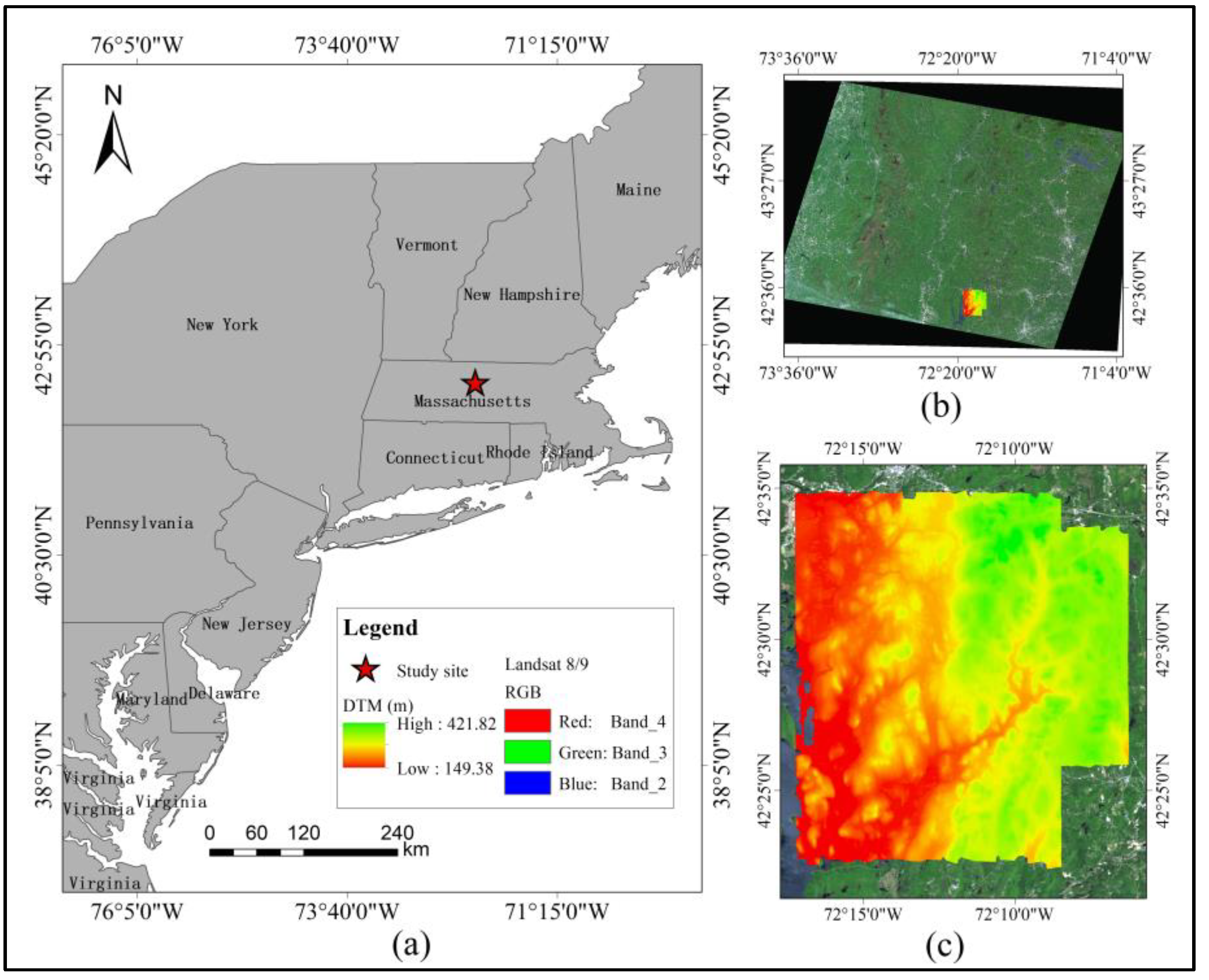
2.1. Research Area

This study selected the Harvard Forest (HARV) as the research area, which is a terrestrial National Ecological Observatory Network (NEON) field observation site, as shown in Figure 1. NEON is a large-scale ecological system research project funded by the US National Science Foundation, aiming to establish an ecological observation network that covers the entire United States. It consist of 47 terrestrial sites, 34 freshwater sites, and 4 marine sites [40].

HARV is located approximately 65 miles west of Boston, Massachusetts in the county of Worcester, with an average elevation of 348 m, an annual average temperature of 7.4 °C, and an annual average precipitation of 1080 mm. The dominant vegetation consists of regenerating eastern deciduous forest, composed of red oak (Quercus rubra), red maple (Acer rubrum), and white pine (Pinus strobus), with sublayers of shrubs, trees, ferns, and flowering herbaceous plants that are more common in humid areas.

2.2. Data Acquisition and Processing

2.2.1. ALS Data Processing

The ALS data used in the study were obtained from NEON field observation stations in August 2022. The digital terrain model (DTM) and digital surface model (DSM) extracted from ALS data were verified with field measurements [41], with a spatial resolution of 1 m and horizontal and vertical accuracies of 5–15 cm and 5–35 cm, respectively. The DTM incorporates height information of the ground and other surface objects, facilitating a more precise depiction of the overall terrain. The canopy height model (CHM) is derived by subtracting the DTM from the DSM [42], enabling the isolation of vegetation height while mitigating the impact of terrain and other surface characteristics. Considering the GEDI footprint size of approximately 25 m, the initial DTM and CHM were resampled to 25 m, with the former representing the mean value (DTMmean) and the latter representing the 90th percentile value (RH90) [43], to evaluate the accuracy of GEDI L2A data in retrieving ground elevation and forest canopy height. Moreover, RH90 was employed to assess the performance of the BP neural network models developed in this study for accurately estimating forest canopy height. Figure 2 shows the resampled DTM and CHM imagery.

2.2.2. GEDI L2A Data Processing

The GEDI satellite was launched on 5 December 2018, consisting of three high-precision laser instruments operating at a frequency of 242 Hz, with two operating in full-power mode and one in cover mode. The cover and full-power beams can penetrate 95% and 98% of forest canopies to reach the ground, respectively, producing four ground tracks each, for a total of eight ground observation tracks [44].

Table 1. GEDI parameters [44].

Parameter Name	Parameter Size
Track height	400 km
Coverage	51.6° N–51.6° S
Repetition rate	242 Hz
Pulse width	15 ns
Wavelength	1064 nm
Footprint	25 m
Geolocation error	8 m
Along-track distances	60 m
Across-track distances	600 m

records the relevant parameters and description information of GEDI.

On the basis of research objectives and the time range of data distribution, this study used GEDI L2A version 2 data for ground elevation and forest canopy height retrieval [43]. The data acquisition information is shown in

Table 2. GEDI L2A data acquisition information.

Study Area	Acquisition Date	File Size (GB)
HARV	4 July 2022	2.05
	8 July 2022	2.35
	14 July 2022	2.49
	3 August 2022	2.37
	9 August 2022	2.22
	26 August 2022	2.20
	2 September 2022	2.70
	6 September 2022	1.92
	23 September 2022	2.37
	27 September 2022	2.28

and provided in HDF5 format, available at https://search.earthdata.nasa.gov/search?q=GEDI (accessed on 10 May 2023).

To reduce the impact of adverse conditions such as low-energy ground reflections or high background noise, the produced GEDI L2A elevation data may contain errors. This issue is addressed by setting six sets of noise thresholds, signal thresholds, signal start thresholds, and signal end thresholds for the GEDI L1B datasets (

Table 3. GEDI L2A algorithm setting groups. σ represents the standard deviation of the background noise level [45].

Algorithm Setting Group	Smoothing Width (Noise)	Smoothing Width (Signal)	Waveform Signal Start Threshold	Waveform Signal End Threshold
a1	6.5σ	6.5σ	3σ	6σ
a2	6.5σ	3.5σ	3σ	3σ
a3	6.5σ	3.5σ	3σ	6σ
a4	6.5σ	6.5σ	6σ	6σ
a5	6.5σ	3.5σ	3σ	2σ
a6	6.5σ	3.5σ	3σ	4σ

). Gaussian filters are utilized to enhance the measurement accuracy of GEDI L2A data under various weather conditions and geographical environments by smoothing the waveforms [45].

In this study, four tracks of GEDI full-power waveform data were chosen, and specific criteria were applied for footprint screening: ‘quality_flag’ = 1, ‘degrade_flag’ = 0, and ‘sensitivity’ ≥ 0.9 [41,46]. A total of 1861 high-quality footprints were selected for HARV site (Figure 3). The ‘elev_lowestmode’ and ‘rh’ parameters of the GEDI L2A data were extracted from these GEDI footprints, and all footprints, represented by red dots and green dots, were utilized to verify the ground elevation and forest canopy height. Additionally, these footprints were randomly assigned, with 80% of the footprints used for training the BP neural network forest canopy height retrieval model (red points) and 20% for testing the retrieval performance of the model (green points).

2.2.3. Landsat 8 and 9 Data Processing

Landsat 9 is the ninth satellite in the US Landsat program. It was launched on 27 September 2021, and orbits jointly with Landsat 8, providing observations every 8 days. It carries the OLI-2, a second-generation land imager with nine spectral bands, which captures observations of the Earth’s surface in visible, near-infrared, and shortwave infrared bands. The radiometric measurement accuracy has been improved from Landsat 8 OLI’s 12-bit to 14-bit quantization, and the overall signal-to-noise ratio has been slightly increased, enabling the detection of more biological information in dense forests [47]. The satellite parameters are shown in

Table 4. Parameters of Operational Land Imager 2 sensor.

Band Name	Band Range (μm)	Spatial Resolution (m)
Band 1 Coastal	0.43–0.45	30
Band 2 Blue	0.45–0.51	30
Band 3 Green	0.53–0.59	30
Band 4 Red	0.64–0.67	30
Band 5 NIR	0.85–0.88	30
Band 6 SWIR 1	1.57–1.65	30
Band 7 SWIR 2	2.11–2.29	30
Band 8 PAN	0.50–0.68	15
Band 9 Cirrus	1.36–1.38	30

.

According to the acquisition time and weather conditions of the ALS data, Landsat 8 and 9 satellite imagery were selected for this study, as shown in

Table 5. Landsat data acquisition information.

Sensor	Path/Row	Study Area	Acquisition Date
OLI	013/030	HARV	6 August 2022
OLI-2	013/030		14 August 2022

. The HARV study area was meticulously selected to ensure a cloud-free environment, guaranteeing unobstructed visibility for the analysis (refer to Figure 4). The selected Landsat 8 and 9 satellite imagery used in this study are Level-1T products, meticulously corrected for terrain distortions. To obtain accurate surface reflectance, the remote-sensing images underwent radiometric calibration, converting the grayscale values to radiance values using Equation (1). Furthermore, the FLAASH module in ENVI was employed to perform atmospheric correction, converting the radiance values to actual surface reflectance [48].

$$L=\frac{DN}{\mathrm{a}}+L_0$$

(1)

In the Equation (1), L represents radiance, DN represents the grayscale value of the sensor, and a and L₀ are from the satellite data file, representing the gain and offset values, respectively.

2.3. Forest Canopy Height Inversion Model Construction

2.3.1. BP Neural Network

BP neural networks are extensively employed in supervised learning tasks, effectively adjusting weights through backpropagation to minimize loss [49]. The process encompasses network initialization, forward propagation, loss calculation, backpropagation, and weight updating [50,51]. Notably proficient in classification and regression, they necessitate meticulous attention to network structure, hyperparameters, and adversities like vanishing gradients [52]. Diverging from traditional networks, they leverage backpropagation, non-linear activation functions, multiple layers, augmented expressiveness, and improved training efficiency [53]. These facets bolster their eminence in neural network applications.

2.3.2. Activation Function

Activation functions serve to overcome the limitations of linear models by introducing non-linear components that enhance the expressiveness of the models [54,55]. Three types of activation functions are commonly used in BP neural networks: logistic Equation (2), ReLU Equation (3), and tanh Equation (4).

$$\log istic=\frac{1}{1+e^{-x}}$$

(2)

The logistic takes values between 0 and 1, is monotonic and continuous, and is everywhere differentiable, with near-saturation zones on the left and right, which can easily cause the gradient to disappear [56,57,58]. Special care should be taken when initializing the weight matrix to prevent saturation from causing the network to barely learn.

$$\mathrm{Re}LU(x)=\{\begin{array}{c}0\\ x\end{array}\begin{array}{c}x<0\\ x>=0\end{array}$$

(3)

The output of ReLU is still non-zero symmetric, has no exponential operations compared with logistic, is computationally simple and efficient, converges faster, does not saturate in the positive interval direction, and can solve the problem of vanishing gradients [59,60].

$$\tanh (x)=\frac{e^x-e^{-x}}{e^x+e^{-x}}$$

(4)

The tanh takes values between −1 and 1, is monotonically continuous, is everywhere differentiable, has an approximate saturation zone, and has a larger range and faster convergence than logistic because the slope is greater in the region around 0, which speeds up the convergence [57,61]. ReLU effectively addresses the vanishing gradient problem, speeds up computation, and promotes sparse representation. These qualities enhance training efficiency and improve the expressive power of the neural network. ReLU activation function is selected for the BP neural network model due to its advantageous properties in this study.

2.3.3. Determination of the Number of Neurons in the Hidden Layer

Choosing the appropriate number of neurons in the hidden layer is crucial in achieving optimal performance in a neural network. Insufficient neurons can result in underfitting, where the model fails to capture complex patterns and exhibits poor performance [62,63]. A larger number of neurons can increase the model’s capacity to learn intricate relationships in the data, but it may also increase the risk of overfitting [64]. The determination of the number of neurons in the hidden layer is derived from the empirical Equation (5) [65]:

$$Q=\sqrt{m+n}+\alpha$$

(5)

where the Q is the number of hidden layer neurons, m is the number of input layer features, n is the number of output layers, and α takes values between 0 and 10.

2.3.4. Independent Variables Extraction

Multi-spectral data, with their diverse spectral characteristics and vegetation indices, along with LiDAR data, are both pivotal for accurately estimating forest canopy height [66]. Multi-spectral data capture a wide range of spectral information, offering valuable insights into vegetation health and structure. They enable the calculation of various vegetation indices that aid in canopy height estimation. LiDAR data employ laser pulses to directly measure canopy height, ensuring precise and reliable measurements. Integrating these data types yields a comprehensive and accurate estimation of forest canopy height [66,67]. The construction of remote-sensing indicators is a prerequisite and key step for canopy height retrieval [68]. Different types and sources of feature variables reflect the differences in retrieval targets from different dimensions. Based on the relevant literature [69,70,71], this study focuses on extracting multiple relative heights from GEDI L2A data and multiple vegetation indices from Landsat 8 and 9 data (

Table 6. Summary of metrics computed from GEDI L2A data and Landsat data.

Independent Variable	Variable Information	References
rh25, rh50, rh60, rh75, rh85, rh90, rh95, rh100	Relative height metrics at (25, 50, 60, 75, 85, 90, 95, 100)%	–
EVI	$EVI=2.5*\left(\frac{B5 - B4}{B5 + 6 * B4 - 7 * B2 + 1}\right)$	[73]
NDVI	$NDVI=\left(B5-B4\right)/\left(B5+B4\right)$	[74]
SAVI	$SAVI=\frac{\left(1 + L\right)\left(B5 - B4\right)}{B5 + B4 + L}\left(L=0.5\right)$	[75]
SLAVI	$SLAVI=\frac{B5}{B4 + B7}$	[76]
RVI	$RVI=B5/B4$	[77]
VI3	$VI3=\frac{B3}{B4 + B5}$	[78]
PVI	$PVI=\frac{(B5 - a * B4 - b)}{(\sqrt{1 + a^2})}{(}_{b - gradient of the soil line}^{a - slope of the soil line})$	[79]
SARVI	$\left(1+L\right)\frac{B5 - 2 * B4 + B2}{\left(B5 + 2 * B4 - B2 + L\right)}\left(L=0.5\right)$	[80]
DVI	$DVI=B5-B4$	[81]
ARVI	$ARVI=\frac{B5 - 2 * B4 + B2}{B5 + 2 * B4 - B2}$	[80]
TCG	Greenness of TCT	[82]
TCB	Brightness of TCT	[82]
TCW	Wetness of TCT	[82]

). The extracted variables are then filtered using importance scores and input into a BP neural network model to achieve forest canopy height inversion. Considering the disparate resolutions of Landsat imagery, GEDI L2A, and ALS data, this study employs the center coordinates of GEDI footprints as a reference for variable extraction [72]. This methodology guarantees the alignment and comparability of extracted variables, effectively addressing the challenge posed by resolution differences in the data sources.

2.3.5. Importance Analysis of Independent Variables

Feature dimensionality reduction through variable selection is a critical aspect of machine learning that significantly improves computational efficiency. In this study, the random forest algorithm was employed to determine the importance scores of each feature, quantifying their contributions to individual trees within the random forest ensemble. These scores were then averaged and ranked to identify the most influential features. The analysis focused on the HARV study area, utilizing a dataset of 1861 samples for random forest model training.

The importance scores revealed that the GEDI relative height feature exhibited high sensitivity to forest canopy height, consistently outperforming the Landsat vegetation index feature (refer to Figure 5). For model construction, the top variables with a cumulative contribution of 90% were selected to reduce the dimensionality of the feature set (red bars in Figure 5). This approach effectively retained the essential information required for accurate forest canopy height predictions while reducing computational complexity.

After filtering the features based on their importance scores, a control experiment was conducted to invert the forest canopy height. In this experiment, the same vegetation index feature variables were selected for both the OLI and OLI-2 models. Similarly, the GEDI and OLI, as well as the GEDI and OLI-2 models, used the same set of feature variables as input (refer to

Table 7. Summary of independent variables for the inverse model.

Model	Independent Variables	Number of Independent Variables
GEDI	rh75, rh60, rh85, rh95, rh100, rh25, rh90	7
OLI/OLI-2	SLAVI, TCB, VI3, EVI, ARVI, TCG, TCW, DVI, PVI	9
GEDI and OLI/OLI-2	rh75, rh60, rh85, rh95, VI3, SLAVI, rh90, rh100, EVI, rh25, rh50, DVI, TCW	13

). This approach ensures consistency and comparability among the different models, enabling a rigorous evaluation of the inversion results. This control experiment helps validate the effectiveness and reliability of the chosen feature variables in the forest canopy height inversion process.

2.3.6. Model Construction

The models utilized in this study incorporate a single hidden layer, striking a delicate balance between complexity and training efficiency, while maintaining exceptional expressive capabilities [83]. The number of neurons Q in the hidden layer of model is calculated by Equation (5).

Table 8. BP neural network model node layer settings.

Data Group	Number of Neurons
	Input Layer	Hidden Layer	Output Layer
GEDI	7	9	1
OLI	9	8	1
OLI-2	9	8	1
GEDI and OLI	13	11	1
GEDI and OLI-2	13	11	1

presents the computed number of hidden layer neurons for each model, which were determined through a combination of 10-fold cross-validation and Python’s grid search. The MLPRegressor function of Python’s sklearn package was used to train the BP neural network forest canopy height inversion model, with a maximum number of 2000 iterations, a learning rate of 0.001, the Adam optimizer, and default values were used for other parameters [84,85,86]. The activation function of the hidden layer was the ReLU, and the output layer function used was the linear function.

2.4. Accuracy Verification Method

The inverse accuracy of ground elevation and forest canopy height was tested using the coefficient of determination (R-squared), absolute mean error (MAE), root mean square error (RMSE), and relative root mean square error (rRMSE). A closer value of R-squared to 1 corresponds to a high model accuracy, and smaller MAE, RMSE and rRMSE correspond to the predicted value of the regression model being closer to the actual measured value. The calculation equations are as follows:

$$R^2=1-\frac{{\displaystyle \sum _{i=1}^m{(y_i-x_i)}^2}}{{\displaystyle \sum _{i=1}^m{(y_i-\overline{y})}^2}}$$

(6)

$$MAE=\frac{1}{m}{\displaystyle \sum _{i=1}^m\left|y_i-x_i\right|}$$

(7)

$$RMSE=\sqrt{\frac{{\displaystyle \sum _{i=1}^m{(y_i-x_i)}^2}}{m}}$$

(8)

$$rRMSE=\frac{100\%}{\overline{y}}\sqrt{\frac{{\displaystyle \sum _{i=1}^m{(y_i-x_i)}^2}}{m}}$$

(9)

where $m$ is the total number of samples, $y_i$ is the validation value, $x_i$ is the predicted value and $\overline{y}$ is the mean of the validation values.

3. Results

3.1. Ground Elevation Inversion Using GEDI L2A Data

The GEDI L2A version 1 data utilize the default algorithm a1 for terrain elevation estimation. However, in version 2 data, the algorithm for terrain elevation estimation varies depending on the type of vegetation function, as specified in Table 3. For densely wooded areas, an algorithm with a lower signal threshold may be preferred to accurately estimate terrain elevation [87].

In the HARV study area, a total of 1861 valid footprints were utilized for accuracy verification to assess the capability of GEDI L2A data in accurately estimating ground elevation and forest canopy height. According to the GEDI L2A algorithms, six sets of footprint point ground elevations were extracted and utilized for conducting control experiments alongside the ALS data. The scatter plot (Figure 6) reveals that algorithm a2 achieved the highest accuracy, with an RMSE of less than 4 m and a rRMSE of approximately 1.5%. Algorithms a1 and a4 demonstrated comparable accuracy because they shared the same signal smoothing width and signal end threshold. However, algorithm a5 exhibited the poorest accuracy, with an RMSE as high as 9.76 m, making it the least accurate among the tested algorithms.

3.2. Forest Canopy Height Inversion Using GEDI L2A Data

The relative height parameter ‘rh’ from the default algorithm of GEDI L2A data was initially extracted. It consisted of 11 height metrics (rh90 to rh100), which indicate the relative height of vegetation at 90% to 100% of the total accumulated energy of the waveform at each footprint. These parameters were then analyzed in comparison to the resampled RH90 derived from the ALS data. The results of this analysis are presented in

Table 9. Comparison of relative height parameters from GEDI L2A default algorithm with ALS-RH90.

Relative Height	Evaluation Indicator
	R-Squared	MAE (m)	RMSE (m)	rRMSE
rh90	0.30	3.66	5.50	24.04%
rh91	0.32	3.58	5.43	23.72%
rh92	0.33	3.51	5.36	23.42%
rh93	0.34	3.45	5.29	23.12%
rh94	0.35	3.41	5.24	22.89%
rh95	0.35	3.41	5.22	22.81%
rh96	0.34	3.44	5.24	22.88%
rh97	0.32	3.54	5.29	23.10%
rh98	0.28	3.71	5.42	23.68%
rh99	0.22	4.07	5.69	24.85%
rh100	0.04	4.95	6.38	27.87%

.

Based on the results presented in Table 9, it is evident that the accuracy of canopy height inversion gradually increases from rh90 to rh95, followed by a decrease from rh95 to rh100. As a result, the rh95 parameter of GEDI L2A data is tentatively considered to be more effective for achieving canopy height inversion. Building on these findings, the study extracted the rh95 values for six different algorithms applied to GEDI L2A data. The subsequent comparison experiment, as shown in Figure 7, demonstrates that algorithm a5 exhibits poor accuracy in canopy height inversion, whereas algorithm a2 consistently achieves the highest level of accuracy.

3.3. BP Neural Network Model Inversion Results

In Figure 3, we divided the sample points into two sets, using 80% for model training and reserving 20% (373 points) for model validation. To enhance model training efficiency and achieve higher accuracy, refer to Table 7 and Table 8 for the chosen model input features and parameter settings. In the HARV study area, we developed three models based on single data sources and two models using combined data sources (refer to Figure 8). Among the single-data models, the GEDI model demonstrated superior accuracy compared to the OLI and OLI-2 models, benefiting from the direct retrieval of forest canopy structural parameters provided by GEDI data, which exhibited higher overall importance scores than subsequent data sources. The OLI-2 data, in comparison to OLI, enabled the detection of denser forests, resulting in increased inversion accuracy with an elevated R-squared of 0.42 and a reduced RMSE of 0.18 m. The joint models showed comparable accuracy but consistently outperformed any single-data model. The optimal GEDI and OLI-2 model (R-squared of 0.75, MAE of 2.20 m, RMSE of 3.11 m, and rRMSE of 13.97%) showcased an enhanced R-squared by 0.37 and a decreased RMSE by 1.81 m compared to the least performing OLI model (R-squared of 0.38, MAE of 3.41 m, RMSE of 4.92 m, and rRMSE of 22.06%). The overestimation of forest canopy height in areas below 10 m may be attributed to limitations in sensor resolution, data noise, inadequate training samples, and flawed model assumptions.

4. Discussion

The GEDI L2A data provide six algorithms (Table 3) to control the waveform length and improve the measurement accuracy of GEDI L2A under different meteorological conditions and geographic environments by changing the waveform signal smoothing width, signal start and signal end thresholds. The signal smoothing width is used to eliminate noise, but a value that is too small cannot effectively remove noise, while a value that is too large can cause signal distortion. The signal start threshold is used to detect the starting position of the signal and affects the highest value of the forest canopy. The signal end threshold is used to obtain the ending position of the signal and affects the lowest value of the ground.

The analysis of various algorithms for GEDI L2A ground elevation reveals that algorithm a2 exhibits the highest accuracy, while algorithm a5 demonstrates the lowest accuracy (refer to Figure 6). Algorithms a1, a3, and a4 have higher signal end thresholds compared to algorithm a2, leading to the detection of higher levels of noise relative to the actual ground, thus resulting in underestimated values for ground elevation. Conversely, algorithm a5 has a lower signal end threshold than algorithm a6, resulting in a wider range of ground elevation detection but lower overall accuracy.

The default algorithm, rh95, for forest canopy height inversion in GEDI L2A data, demonstrates the highest accuracy, consistent with findings from relevant scholarly studies [43,88,89,90]. However, in comparison to their study, there are some factors in our study that could have contributed to less accuracy. Firstly, the sample size in our study was relatively small, which could have limited the representativeness of the data. Additionally, we did not conduct a separate analysis of the GEDI L2A data collected during the day and night, which could have resulted in variations in the accuracy of canopy height estimates. To address these limitations and improve the accuracy of our results, we collected additional samples to ensure temporal consistency between ALS data and GEDI L2A data. This allowed for more precise and reliable estimates of canopy height in the study area. Among the six algorithms extracted from GEDI L2A data and analyzed against airborne data, algorithm a2 exhibits the highest accuracy, while algorithm a5 shows the lowest accuracy. These results align with the outcomes of ground elevation inversion. Algorithm a5, characterized by longer waveform lengths and lower end thresholds, tends to overestimate canopy height. Among the analyzed algorithms, algorithm a2 exhibits waveform lengths comparable to algorithm a5, while delivering more accurate estimations of forest canopy height.

In this paper, five forest canopy height inversion models were developed to estimate forest canopy height in the study area using BP neural network. Compared to the GEDI model, the OLI and OLI-2 models exhibit relatively lower accuracy in the inversion of forest canopy height, which can be attributed to the characteristics of the data used. The analysis of Figure 5 reveals that the importance scores of vegetation indices extracted from OLI-2 data have larger deviations, while those from OLI data are relatively more concentrated. Although the OLI-2 model demonstrates slightly higher accuracy than the OLI model, it is evident that the improvement in data quality offered by OLI-2 can contribute to enhancing the precision of forest canopy height inversion to a certain degree.

Although the combined model of GEDI and Landsat data has yielded successful results, it is crucial to address potential sources of error and uncertainty. Firstly, the BP neural network model used for forest canopy height mapping exhibits inherent uncertainty. The accuracy and representativeness of the training data significantly impact the model’s performance [91,92,93]. Insufficient and incomplete training data can result in inaccurate predictions in unknown scenarios. Overfitting, a common issue in BP neural network models, can lead to excellent performance on training data but poor performance on new data [94,95]. To mitigate overfitting, suitable regularization methods and optimization strategies must be employed. Additionally, the selection of hyperparameters can affect the model’s uncertainty [96].

Furthermore, in our comparative experiments, we chose the same independent variables to facilitate model comparisons. However, this approach may inadvertently exclude variables with high importance scores, leading to reduced prediction accuracy. The calculation of independent variable importance scores was performed using all samples, while only 20% of the samples were used for model validation, potentially introducing inappropriate input features. Moreover, the determination of the number of hidden layers and neurons in the hidden layers based on empirical methods raises the question of their suitability in the current research context.

Future studies should focus on refined independent-variable selection and meticulous exploration of model hyperparameters. These efforts will enhance the understanding and management of uncertainty in the BP neural network model, providing more reliable forest canopy height mapping results and serving as a robust foundation for decision-making and practical applications.

5. Conclusions

Forest canopy height serves as a vital parameter for quantifying forest biomass and carbon storage. GEDI has acquired a substantial amount of global laser point data since its launch. However, data accuracy and reliability are influenced by terrain variations and vegetation cover. Landsat data offers advantages such as high spatial resolution, long time series, and multiple spectral bands, providing detailed surface information. Due to GEDI’s direct retrieval of forest structural parameters, it achieves higher precision in canopy height inversion compared to Landsat data. GEDI and Landsat provide distinct surface feature information, and this study combines both data types to construct a forest canopy height inversion model. The combined model exhibits significantly superior accuracy compared to single-data models, effectively enhancing forest canopy height inversion accuracy. We observed that the practicality of the combined inversion model diminishes when studying smaller regions with limited GEDI footprint coverage. Compared to GEDI, ICESat-2’s laser altimeter enables a higher vertical resolution of approximately 10 cm and offers more ground sampling points. The capability of ICESat-2 in canopy height inversion for forests warrants exploration. In future research, we can extract ground sample points using GEDI and ICESat-2 data, integrate them with optical remote sensing imagery, and construct multiple machine-learning models to achieve large-scale forest canopy height estimation at regional scales. Enhancing the precision of forest canopy height estimation facilitates more accurate assessment of carbon storage and biomass. This advancement enables us to effectively manage and protect valuable forest resources, drive the development of a sustainable green economy, and make significant contributions to addressing the challenges of climate change and achieving sustainable development goals.

References

1. Alexander, C.; Korstjens, A.H.; Hill, R.A. Influence of micro-topography and crown characteristics on tree height estimations in tropical forests based on lidar canopy height models. Int. J. Appl. Earth Obs. Geoinf. 2018, 65, 105–113. [Google Scholar] [CrossRef]
2. Asner, G.P.; Mascaro, J. Mapping tropical forest carbon: Calibrating plot estimates to a simple lidar metric. Remote Sens. Environ. 2014, 140, 614–624. [Google Scholar] [CrossRef]
3. Lucas, R.; Van De Kerchove, R.; Otero, V.; Lagomasino, D.; Fatoyinbo, L.; Omar, H.; Satyanarayana, B.; Dahdouh-Guebas, F. Structural characterisation of mangrove forests achieved through combining multiple sources of remote sensing data. Remote Sens. Environ. 2020, 237, 111543. [Google Scholar] [CrossRef]
4. Tuominen, S.; Eerikäinen, K.; Schibalski, A.; Haakana, M.; Lehtonen, A. Mapping biomass variables with a multi-source forest inventory technique. Silva Fenn. 2010, 44, 109–119. [Google Scholar] [CrossRef] [Green Version]
5. Hu, T.; Su, Y.; Xue, B.; Liu, J.; Zhao, X.; Fang, J.; Guo, Q. Mapping global forest aboveground biomass with spaceborne lidar, optical imagery, and forest inventory data. Remote Sens. 2016, 8, 565. [Google Scholar] [CrossRef] [Green Version]
6. Lefsky, M.A.; Cohen, W.B.; Parker, G.G.; Harding, D.J. Lidar remote sensing for ecosystem studies: Lidar, an emerging remote sensing technology that directly measures the three-dimensional distribution of plant canopies, can accurately estimate vegetation structural attributes and should be of particular interest to forest, landscape, and global ecologists. BioScience 2002, 52, 19–30. [Google Scholar] [CrossRef]
7. Ghosh, A.; Fassnacht, F.E.; Joshi, P.K.; Koch, B. A framework for mapping tree species combining hyperspectral and lidar data: Role of selected classifiers and sensor across three spatial scales. Int. J. Appl. Earth Obs. Geoinf. 2014, 26, 49–63. [Google Scholar] [CrossRef]
8. Jin, S.; Su, Y.; Gao, S.; Hu, T.; Liu, J.; Guo, Q. The transferability of random forest in canopy height estimation from multi-source remote sensing data. Remote Sens. 2018, 10, 1183. [Google Scholar] [CrossRef] [Green Version]
9. Shao, Z.; Zhang, L.; Wang, L. Stacked sparse autoencoder modeling using the synergy of airborne lidar and satellite optical and sar data to map forest above-ground biomass. IEEE J. Sel. Top. Appl. Earth Obs. Remote Sens. 2017, 10, 5569–5582. [Google Scholar] [CrossRef]
10. Klosterman, S.; Melaas, E.; Wang, J.A.; Martinez, A.; Frederick, S.; O’Keefe, J.; Orwig, D.A.; Wang, Z.; Sun, Q.; Schaaf, C.; et al. Fine-scale perspectives on landscape phenology from unmanned aerial vehicle (uav) photography. Agric. For. Meteorol. 2018, 248, 397–407. [Google Scholar] [CrossRef]
11. Lu, B.; He, Y. Species classification using unmanned aerial vehicle (uav)-acquired high spatial resolution imagery in a heterogeneous grassland. ISPRS J. Photogramm. Remote Sens. 2017, 128, 73–85. [Google Scholar] [CrossRef]
12. Kayitakire, F.; Hamel, C.; Defourny, P. Retrieving forest structure variables based on image texture analysis and ikonos-2 imagery. Remote Sens. Environ. 2006, 102, 390–401. [Google Scholar] [CrossRef]
13. Irons, J.R.; Dwyer, J.L.; Barsi, J.A. The next landsat satellite: The landsat data continuity mission. Remote Sens. Environ. 2012, 122, 11–21. [Google Scholar] [CrossRef] [Green Version]
14. Zhu, X.; Wang, C.; Nie, S.; Pan, F.; Xi, X.; Hu, Z. Mapping forest height using photon-counting lidar data and landsat 8 oli data: A case study in virginia and north carolina, USA. Ecol. Indic. 2020, 114, 106287. [Google Scholar] [CrossRef]
15. Wang, Z.; Schaaf, C.B.; Lewis, P.; Knyazikhin, Y.; Schull, M.A.; Strahler, A.H.; Yao, T.; Myneni, R.B.; Chopping, M.J.; Blair, B.J. Retrieval of canopy height using moderate-resolution imaging spectroradiometer (modis) data. Remote Sens. Environ. 2011, 115, 1595–1601. [Google Scholar] [CrossRef] [Green Version]
16. Gupta, P.; Christopher, S.A.; Wang, J.; Gehrig, R.; Lee, Y.; Kumar, N. Satellite remote sensing of particulate matter and air quality assessment over global cities. Atmos. Environ. 2006, 40, 5880–5892. [Google Scholar] [CrossRef]
17. Smith, L.C. Satellite remote sensing of river inundation area, stage, and discharge: A review. Hydrol. Process. 1997, 11, 1427–1439. [Google Scholar] [CrossRef]
18. Kumar, P.; Krishna, A.P. Insar-based tree height estimation of hilly forest using multitemporal radarsat-1 and sentinel-1 sar data. IEEE J. Sel. Top. Appl. Earth Obs. Remote Sens. 2019, 12, 5147–5152. [Google Scholar] [CrossRef]
19. Pourshamsi, M.; Xia, J.; Yokoya, N.; Garcia, M.; Lavalle, M.; Pottier, E.; Balzter, H. Tropical forest canopy height estimation from combined polarimetric sar and lidar using machine-learning. ISPRS J. Photogramm. Remote Sens. 2021, 172, 79–94. [Google Scholar] [CrossRef]
20. Niculescu, S.; Lardeux, C.; Grigoras, I.; Hanganu, J.; David, L. Synergy between lidar, radarsat-2, and spot-5 images for the detection and mapping of wetland vegetation in the danube delta. IEEE J. Sel. Top. Appl. Earth Obs. Remote Sens. 2016, 9, 3651–3666. [Google Scholar] [CrossRef] [Green Version]
21. Mallet, C.; Bretar, F. Full-waveform topographic lidar: State-of-the-art. ISPRS J. Photogramm. Remote Sens. 2009, 64, 1–16. [Google Scholar] [CrossRef]
22. White, J.C.; Wulder, M.A.; Vastaranta, M.; Coops, N.C.; Pitt, D.; Woods, M. The utility of image-based point clouds for forest inventory: A comparison with airborne laser scanning. Forests 2013, 4, 518–536. [Google Scholar] [CrossRef] [Green Version]
23. Wilkes, P.; Jones, S.D.; Suarez, L.; Mellor, A.; Woodgate, W.; Soto-Berelov, M.; Haywood, A.; Skidmore, A.K. Mapping forest canopy height across large areas by upscaling als estimates with freely available satellite data. Remote Sens. 2015, 7, 12563–12587. [Google Scholar] [CrossRef] [Green Version]
24. Ben-Arie, J.R.; Hay, G.J.; Powers, R.P.; Castilla, G.; St-Onge, B. Development of a pit filling algorithm for lidar canopy height models. Comput. Geosci. 2009, 35, 1940–1949. [Google Scholar] [CrossRef]
25. Disney, M.I.; Kalogirou, V.; Lewis, P.; Prieto-Blanco, A.; Hancock, S.; Pfeifer, M. Simulating the impact of discrete-return lidar system and survey characteristics over young conifer and broadleaf forests. Remote Sens. Environ. 2010, 114, 1546–1560. [Google Scholar] [CrossRef]
26. Ma, Q.; Su, Y.; Guo, Q. Comparison of canopy cover estimations from airborne lidar, aerial imagery, and satellite imagery. IEEE J. Sel. Top. Appl. Earth Obs. Remote Sens. 2017, 10, 4225–4236. [Google Scholar] [CrossRef]
27. Verrelst, J.; Rivera, J.P.; Veroustraete, F.; Muñoz-Marí, J.; Clevers, J.G.P.W.; Camps-Valls, G.; Moreno, J. Experimental sentinel-2 lai estimation using parametric, non-parametric and physical retrieval methods—A comparison. ISPRS J. Photogramm. Remote Sens. 2015, 108, 260–272. [Google Scholar] [CrossRef]
28. Li, G.; Xie, Z.; Jiang, X.; Lu, D.; Chen, E. Integration of ziyuan-3 multispectral and stereo data for modeling aboveground biomass of larch plantations in north China. Remote Sens. 2019, 11, 2328. [Google Scholar] [CrossRef] [Green Version]
29. Strahler, A.H. Vegetation canopy reflectance modeling—Recent developments and remote sensing perspectives. Remote Sens. Rev. 1997, 15, 179–194. [Google Scholar] [CrossRef]
30. Stojanova, D.; Panov, P.; Gjorgjioski, V.; Kobler, A.; Džeroski, S. Estimating vegetation height and canopy cover from remotely sensed data with machine learning. Ecol. Inform. 2010, 5, 256–266. [Google Scholar] [CrossRef]
31. Massman, W. A comparative study of some mathematical models of the mean wind structure and aerodynamic drag of plant canopies. Bound. Layer Meteorol. 1987, 40, 179–197. [Google Scholar] [CrossRef]
32. Pittman, J.J.; Arnall, D.B.; Interrante, S.M.; Moffet, C.A.; Butler, T.J. Estimation of biomass and canopy height in bermudagrass, alfalfa, and wheat using ultrasonic, laser, and spectral sensors. Sensors 2015, 15, 2920–2943. [Google Scholar] [CrossRef] [Green Version]
33. Verstraete, M.M.; Pinty, B.; Myneni, R.B. Potential and limitations of information extraction on the terrestrial biosphere from satellite remote sensing. Remote Sens. Environ. 1996, 58, 201–214. [Google Scholar] [CrossRef]
34. Pourshamsi, M.; Garcia, M.; Lavalle, M.; Balzter, H. A machine-learning approach to polinsar and lidar data fusion for improved tropical forest canopy height estimation using nasa afrisar campaign data. IEEE J. Sel. Top. Appl. Earth Obs. Remote Sens. 2018, 11, 3453–3463. [Google Scholar] [CrossRef] [Green Version]
35. Han, T.; Jiang, D.; Zhao, Q.; Wang, L.; Yin, K. Comparison of random forest, artificial neural networks and support vector machine for intelligent diagnosis of rotating machinery. Trans. Inst. Meas. Control 2018, 40, 2681–2693. [Google Scholar] [CrossRef]
36. Rodriguez-Galiano, V.; Sanchez-Castillo, M.; Chica-Olmo, M.; Chica-Rivas, M. Machine learning predictive models for mineral prospectivity: An evaluation of neural networks, random forest, regression trees and support vector machines. Ore Geol. Rev. 2015, 71, 804–818. [Google Scholar] [CrossRef]
37. Otchere, D.A.; Arbi Ganat, T.O.; Gholami, R.; Ridha, S. Application of supervised machine learning paradigms in the prediction of petroleum reservoir properties: Comparative analysis of ann and svm models. J. Pet. Sci. Eng. 2021, 200, 108182. [Google Scholar] [CrossRef]
38. Alzubaidi, L.; Zhang, J.; Humaidi, A.J.; Al-Dujaili, A.; Duan, Y.; Al-Shamma, O.; Santamaría, J.; Fadhel, M.A.; Al-Amidie, M.; Farhan, L. Review of deep learning: Concepts, cnn architectures, challenges, applications, future directions. J. Big Data 2021, 8, 53. [Google Scholar] [CrossRef] [PubMed]
39. Cao, H.; Han, L.; Li, L. Harmonizing surface reflectance between landsat-7 etm+, landsat-8 oli, and sentinel-2 msi over China. Environ. Sci. Pollut. Res. 2022, 29, 70882–70898. [Google Scholar] [CrossRef] [PubMed]
40. Scholl, V.M.; Cattau, M.E.; Joseph, M.B.; Balch, J.K. Integrating national ecological observatory network (neon) airborne remote sensing and in-situ data for optimal tree species classification. Remote Sens. 2020, 12, 1414. [Google Scholar] [CrossRef]
41. Liu, A.; Cheng, X.; Chen, Z. Performance evaluation of gedi and icesat-2 laser altimeter data for terrain and canopy height retrievals. Remote Sens. Environ. 2021, 264, 112571. [Google Scholar] [CrossRef]
42. White, J.C.; Coops, N.C.; Wulder, M.A.; Vastaranta, M.; Hilker, T.; Tompalski, P. Remote sensing technologies for enhancing forest inventories: A review. Can. J. Remote Sens. 2016, 42, 619–641. [Google Scholar] [CrossRef] [Green Version]
43. Potapov, P.; Li, X.; Hernandez-Serna, A.; Tyukavina, A.; Hansen, M.C.; Kommareddy, A.; Pickens, A.; Turubanova, S.; Tang, H.; Silva, C.E.; et al. Mapping global forest canopy height through integration of gedi and landsat data. Remote Sens. Environ. 2021, 253, 112165. [Google Scholar] [CrossRef]
44. Dubayah, R.; Blair, J.B.; Goetz, S.; Fatoyinbo, L.; Hansen, M.; Healey, S.; Hofton, M.; Hurtt, G.; Kellner, J.; Luthcke, S.; et al. The global ecosystem dynamics investigation: High-resolution laser ranging of the earth’s forests and topography. Sci. Remote Sens. 2020, 1, 100002. [Google Scholar] [CrossRef]
45. Adam, M.; Urbazaev, M.; Dubois, C.; Schmullius, C. Accuracy assessment of gedi terrain elevation and canopy height estimates in european temperate forests: Influence of environmental and acquisition parameters. Remote Sens. 2020, 12, 3948. [Google Scholar] [CrossRef]
46. Urbazaev, M.; Hess, L.L.; Hancock, S.; Sato, L.Y.; Ometto, J.P.; Thiel, C.; Dubois, C.; Heckel, K.; Urban, M.; Adam, M.; et al. Assessment of terrain elevation estimates from icesat-2 and gedi spaceborne lidar missions across different land cover and forest types. Sci. Remote Sens. 2022, 6, 100067. [Google Scholar] [CrossRef]
47. Masek, J.G.; Wulder, M.A.; Markham, B.; McCorkel, J.; Crawford, C.J.; Storey, J.; Jenstrom, D.T. Landsat 9: Empowering open science and applications through continuity. Remote Sens. Environ. 2020, 248, 111968. [Google Scholar] [CrossRef]
48. Watanabe, F.S.Y.; Alcântara, E.; Rodrigues, T.W.P.; Imai, N.N.; Barbosa, C.C.F.; Rotta, L.H.d.S. Estimation of chlorophyll-a concentration and the trophic state of the barra bonita hydroelectric reservoir using oli/landsat-8 images. Int. J. Environ. Res. Public Health 2015, 12, 10391–10417. [Google Scholar] [CrossRef] [Green Version]
49. Goh, A.T.C. Back-propagation neural networks for modeling complex systems. Artif. Intell. Eng. 1995, 9, 143–151. [Google Scholar] [CrossRef]
50. Zhang, G.; Xia, B.; Wang, J. Intelligent state of charge estimation of lithium-ion batteries based on l-m optimized back-propagation neural network. J. Energy Storage 2021, 44, 103442. [Google Scholar] [CrossRef]
51. Poorani, S.; Balasubramanie, P. Seizure detection based on eeg signals using asymmetrical back propagation neural network method. Circuits Syst. Signal Process. 2021, 40, 4614–4632. [Google Scholar] [CrossRef]
52. Hochreiter, S. The vanishing gradient problem during learning recurrent neural nets and problem solutions. Int. J. Uncertain. Fuzziness Knowl. Based Syst. 1998, 6, 107–116. [Google Scholar] [CrossRef] [Green Version]
53. Lee, D.-H.; Kim, Y.-T.; Lee, S.-R. Shallow landslide susceptibility models based on artificial neural networks considering the factor selection method and various non-linear activation functions. Remote Sens. 2020, 12, 1194. [Google Scholar] [CrossRef] [Green Version]
54. Varshney, M.; Singh, P. Optimizing nonlinear activation function for convolutional neural networks. Signal Image Video Process. 2021, 15, 1323–1330. [Google Scholar] [CrossRef]
55. Chen, J.-C.; Wang, Y.-M. Comparing activation functions in modeling shoreline variation using multilayer perceptron neural network. Water 2020, 12, 1281. [Google Scholar] [CrossRef]
56. Lederer, J. Activation functions in artificial neural networks: A systematic overview. arXiv 2021, arXiv:2101.09957. [Google Scholar] [CrossRef]
57. Dubey, S.R.; Singh, S.K.; Chaudhuri, B.B. Activation functions in deep learning: A comprehensive survey and benchmark. Neurocomputing 2022, 503, 92–108. [Google Scholar] [CrossRef]
58. Tu, J.V. Advantages and disadvantages of using artificial neural networks versus logistic regression for predicting medical outcomes. J. Clin. Epidemiol. 1996, 49, 1225–1231. [Google Scholar] [CrossRef]
59. Mastromichalakis, S. Alrelu: A different approach on leaky relu activation function to improve neural networks performance. arXiv 2020, arXiv:2012.07564. [Google Scholar] [CrossRef]
60. Alhassan, A.M.; Zainon, W.M.N.W. Brain tumor classification in magnetic resonance image using hard swish-based relu activation function-convolutional neural network. Neural Comput. Appl. 2021, 33, 9075–9087. [Google Scholar] [CrossRef]
61. Misra, D. Mish: A self regularized non-monotonic activation function. arXiv 2019, arXiv:1908.08681. [Google Scholar] [CrossRef]
62. Göçken, M.; Özçalıcı, M.; Boru, A.; Dosdoğru, A.T. Integrating metaheuristics and artificial neural networks for improved stock price prediction. Expert Syst. Appl. 2016, 44, 320–331. [Google Scholar] [CrossRef]
63. Xiao, Y.; Wu, J.; Lin, Z.; Zhao, X. A deep learning-based multi-model ensemble method for cancer prediction. Comput. Methods Programs Biomed. 2018, 153, 1–9. [Google Scholar] [CrossRef] [PubMed]
64. Li, H.; Zhao, W.; Zhang, Y.; Zio, E. Remaining useful life prediction using multi-scale deep convolutional neural network. Appl. Soft Comput. 2020, 89, 106113. [Google Scholar] [CrossRef]
65. Zhu, W.-D.; Qian, C.-Y.; He, N.-Y.; Kong, Y.-X.; Zou, Z.-Y.; Li, Y.-W. Research on chlorophyll-a concentration retrieval based on bp neural network model—Case study of dianshan lake, China. Sustainability 2022, 14, 8894. [Google Scholar] [CrossRef]
66. Ota, T.; Ahmed, O.S.; Franklin, S.E.; Wulder, M.A.; Kajisa, T.; Mizoue, N.; Yoshida, S.; Takao, G.; Hirata, Y.; Furuya, N.; et al. Estimation of airborne lidar-derived tropical forest canopy height using landsat time series in cambodia. Remote Sens. 2014, 6, 10750–10772. [Google Scholar] [CrossRef] [Green Version]
67. Lee, W.-J.; Lee, C.-W. Forest canopy height estimation using multiplatform remote sensing dataset. J. Sens. 2018, 2018, 1593129. [Google Scholar] [CrossRef] [Green Version]
68. Peng, D.; Zhang, H.; Liu, L.; Huang, W.; Huete, A.R.; Zhang, X.; Wang, F.; Yu, L.; Xie, Q.; Wang, C.; et al. Estimating the aboveground biomass for planted forests based on stand age and environmental variables. Remote Sens. 2019, 11, 2270. [Google Scholar] [CrossRef] [Green Version]
69. Bye, I.J.; North, P.R.J.; Los, S.O.; Kljun, N.; Rosette, J.A.B.; Hopkinson, C.; Chasmer, L.; Mahoney, C. Estimating forest canopy parameters from satellite waveform lidar by inversion of the flight three-dimensional radiative transfer model. Remote Sens. Environ. 2017, 188, 177–189. [Google Scholar] [CrossRef] [Green Version]
70. Koetz, B.; Morsdorf, F.; Sun, G.; Ranson, K.J.; Itten, K.; Allgower, B. Inversion of a lidar waveform model for forest biophysical parameter estimation. IEEE Geosci. Remote Sens. Lett. 2006, 3, 49–53. [Google Scholar] [CrossRef]
71. Staben, G.; Lucieer, A.; Scarth, P. Modelling lidar derived tree canopy height from landsat tm, etm+ and oli satellite imagery—A machine learning approach. Int. J. Appl. Earth Obs. Geoinf. 2018, 73, 666–681. [Google Scholar] [CrossRef]
72. Campbell, M.J.; Dennison, P.E.; Kerr, K.L.; Brewer, S.C.; Anderegg, W.R.L. Scaled biomass estimation in woodland ecosystems: Testing the individual and combined capacities of satellite multispectral and lidar data. Remote Sens. Environ. 2021, 262, 112511. [Google Scholar] [CrossRef]
73. Huete, A.; Didan, K.; Miura, T.; Rodriguez, E.P.; Gao, X.; Ferreira, L.G. Overview of the radiometric and biophysical performance of the modis vegetation indices. Remote Sens. Environ. 2002, 83, 195–213. [Google Scholar] [CrossRef]
74. Rouse, J.W.; Haas, R.H.; Schell, J.A.; Deering, D.W. Monitoring Vegetation Systems in the Great Plains with ERTS; NASA Special Publication; NASA: Washington, DC, USA, 1974; Volume 351, p. 309. [Google Scholar]
75. Huete, A.R. A soil-adjusted vegetation index (savi). Remote Sens. Environ. 1988, 25, 295–309. [Google Scholar] [CrossRef]
76. Lymburner, L.; Beggs, P.J.; Jacobson, C.R. Estimation of canopy-average surface-specific leaf area using landsat tm data. Photogramm. Eng. Remote Sens. 2000, 66, 183–192. [Google Scholar]
77. Jordan, C.F. Derivation of leaf-area index from quality of light on the forest floor. Ecology 1969, 50, 663–666. [Google Scholar] [CrossRef]
78. Viña, A. Remote Detection of Biophysical Properties of Plant Canopies. 2002. Available online: http://calmaps.unl.edu/snrscoq/snrs_colloquium_2002_andres_vina.ppt (accessed on 16 May 2003).
79. Richardson, A.J.; Wiegand, C. Distinguishing vegetation from soil background information. Photogramm. Eng. Remote Sens. 1977, 43, 1541–1552. [Google Scholar]
80. Huete, A.R.; Liu, H.Q. An error and sensitivity analysis of the atmospheric- and soil-correcting variants of the ndvi for the modis-eos. IEEE Trans. Geosci. Remote Sens. 1994, 32, 897–905. [Google Scholar] [CrossRef]
81. Tucker, C.J. Red and photographic infrared linear combinations for monitoring vegetation. Remote Sens. Environ. 1979, 8, 127–150. [Google Scholar] [CrossRef] [Green Version]
82. Huang, C.; Wylie, B.; Yang, L.; Homer, C.; Zylstra, G. Derivation of a tasselled cap transformation based on landsat 7 at-satellite reflectance. Int. J. Remote Sens. 2002, 23, 1741–1748. [Google Scholar] [CrossRef]
83. Guliyev, N.J.; Ismailov, V.E. A single hidden layer feedforward network with only one neuron in the hidden layer can approximate any univariate function. Neural Comput. 2016, 28, 1289–1304. [Google Scholar] [CrossRef] [Green Version]
84. Chugh, S.; Ghosh, S.; Gulistan, A.; Rahman, B.M.A. Machine learning regression approach to the nanophotonic waveguide analyses. J. Light. Technol. 2019, 37, 6080–6089. [Google Scholar] [CrossRef] [Green Version]
85. Feng, X.; Ma, G.; Su, S.-F.; Huang, C.; Boswell, M.K.; Xue, P. A multi-layer perceptron approach for accelerated wave forecasting in lake michigan. Ocean Eng. 2020, 211, 107526. [Google Scholar] [CrossRef]
86. Baressi Šegota, S.; Anđelić, N.; Kudláček, J.; Čep, R. Artificial neural network for predicting values of residuary resistance per unit weight of displacement. Pomor. Zb. 2019, 57, 9–22. [Google Scholar]
87. Dubayah, R.; Hofton, M.; Blair, J.; Armston, J.; Tang, H.; Luthcke, S. Gedi l2a Elevation and Height Metrics Data Global Footprint Level v001; NASA EOSDIS Land Processes DAAC: Sioux Falls, SD, USA, 2020. [Google Scholar] [CrossRef]
88. Wang, C.; Elmore, A.J.; Numata, I.; Cochrane, M.A.; Shaogang, L.; Huang, J.; Zhao, Y.; Li, Y. Factors affecting relative height and ground elevation estimations of gedi among forest types across the conterminous USA. GISci. Remote Sens. 2022, 59, 975–999. [Google Scholar] [CrossRef]
89. Dorado-Roda, I.; Pascual, A.; Godinho, S.; Silva, C.A.; Botequim, B.; Rodríguez-Gonzálvez, P.; González-Ferreiro, E.; Guerra-Hernández, J. Assessing the accuracy of gedi data for canopy height and aboveground biomass estimates in mediterranean forests. Remote Sens. 2021, 13, 2279. [Google Scholar] [CrossRef]
90. Wang, C.; Elmore, A.J.; Numata, I.; Cochrane, M.A.; Lei, S.; Hakkenberg, C.R.; Li, Y.; Zhao, Y.; Tian, Y. A framework for improving wall-to-wall canopy height mapping by integrating gedi lidar. Remote Sens. 2022, 14, 3618. [Google Scholar] [CrossRef]
91. Guo, Z.-H.; Wu, J.; Lu, H.-Y.; Wang, J.-Z. A case study on a hybrid wind speed forecasting method using bp neural network. Knowl. Based Syst. 2011, 24, 1048–1056. [Google Scholar] [CrossRef]
92. Li, G.; Shi, J. On comparing three artificial neural networks for wind speed forecasting. Appl. Energy 2010, 87, 2313–2320. [Google Scholar] [CrossRef]
93. Yu, W.; Li, B.; Jia, H.; Zhang, M.; Wang, D. Application of multi-objective genetic algorithm to optimize energy efficiency and thermal comfort in building design. Energy Build. 2015, 88, 135–143. [Google Scholar] [CrossRef]
94. Guresen, E.; Kayakutlu, G.; Daim, T.U. Using artificial neural network models in stock market index prediction. Expert Syst. Appl. 2011, 38, 10389–10397. [Google Scholar] [CrossRef]
95. Lee, D.; Derrible, S.; Pereira, F.C. Comparison of four types of artificial neural network and a multinomial logit model for travel mode choice modeling. Transp. Res. Rec. 2018, 2672, 101–112. [Google Scholar] [CrossRef] [Green Version]
96. Xu, Y.; Huang, Y.; Ma, G. A beetle antennae search improved bp neural network model for predicting multi-factor-based gas explosion pressures. J. Loss Prev. Process Ind. 2020, 65, 104117. [Google Scholar] [CrossRef]
Figure 1. Geographical location of the research area: (a) research area location; (b) the location of HARV on Landsat 8/9 imagery; and (c) HARV topographic map.
Sustainability 15 10434 g001
Figure 2. The DTM and CHM imagery of the HARV area: (a) the DTM imagery before resampling; (b) the DTM imagery after resampling; (c) the CHM imagery before resampling; and (d) the CHM imagery after resampling.
Sustainability 15 10434 g002
Figure 3. Distribution of GEDI footprints in the HARV study area.
Sustainability 15 10434 g003
Figure 4. Landsat 8 (a) and Landsat 9 (b) satellite imagery (red squares indicate the location of the HARV study area in Landsat satellite imagery).
Sustainability 15 10434 g004
Figure 5. Variable importance scores in HARV study area: (a) is the result of independent variables selection from GEDI L2A data; (b) is the result of independent variables selection from Landsat 8 data; (c) is the result of independent variables selection from Landsat 9 data; (d) is the result of independent variables selection from GEDI L2A and Landsat 8 data; and (e) is the result of independent variables selection from GEDI L2A and Landsat 9 data (red bars indicate variables with a cumulative importance score of 90% and the green bars indicate additional variables).
Sustainability 15 10434 g005
Figure 6. Scatterplot of GEDI-DTM estimates and the ALS-DTM of GEDI footprints (a1a6: six algorithms representing GEDI L2A data).
Sustainability 15 10434 g006
Figure 7. Scatterplot of the 95% relative height parameter from GEDI L2A and ALS-RH90 (a1a6: six algorithms representing GEDI L2A data).
Sustainability 15 10434 g007
Figure 8. Estimation of forest canopy height based on BP neural network models: (a) GEDI model; (b) OLI model; (c) OLI-2 model; (d) GEDI and OLI model; and (e) GEDI and OLI-2 model.
Sustainability 15 10434 g008