Abstract
Amid the context of a sustainable development strategy, there is a growing interest in renewable energy as an alternative to traditional energy sources. However, as the penetration rate of clean energy gradually increases, its inherent features, such as randomness and uncertainty, have led to a surging demand for flexibility and regulation in power systems, highlighting the need to enhance the flexibility of power systems in multiple dimensions. This paper proposes a method for evaluating the adjustable power capacity of a virtual power plant (VPP), which considers the high-energy-consuming industrial load in the day-ahead to real-time stages and establishes an optimization scheduling model for auxiliary service markets based on this method. Firstly, within the day-ahead phase, the VPP is categorized and modeled based on its level of load flexibility regulation. The assessable capacity is then evaluated to establish the adjustable power range of the VPP, and the capacity of the VPP is subsequently reported. Secondly, the adjustable loads inside the VPP are ranked using the performance indicator evaluation method to obtain the adjustment order of internal resources. Finally, on the real-time scale, an optimization scheduling model to minimize the net operating cost of the VPP is established based on real-time peak-shaving and frequency regulation instructions from the auxiliary service market and solved using the CPLEX solver. The case study results show that the proposed method effectively reduces the net operating cost of the VPP and improves the stability of its participation in the auxiliary service market, which verifies the effectiveness of the proposed method.
1. Introduction
With the implementation of the “double carbon” national strategy, the utilization of clean energy has become the cornerstone of China’s future energy strategy [1]. Despite this, the inherent characteristics of clean energy, such as high unpredictability, significant short-term fluctuations, and challenging predictability have resulted in substantial wind and solar power curtailment, leading to increased complexity and vulnerability of the power system [2,3]. As a result, research on enhancing power systems’ flexibility and understanding their stable operation mechanism has become a new focus of investigation [4].
In recent years, VPPs that coordinate and control various types of demand-side flexibility resources have become a hot research topic. They can promote resource cooperation, improve the economy and flexibility of demand-side operation, and enhance the integration of renewable energy sources [5,6]. Several studies have modeled VPPs by aggregating different energy resources and applying optimization methods to schedule their operation. In [7], a multi-objective optimization model for VPP scheduling incorporated wind power, photovoltaic power, electric vehicle fleet, and conventional power plants was developed. In [8], conditional value-at-risk and confidence level theory were introduced to establish a scheduling model that includes wind turbines, photovoltaic generators, conventional gas turbines, energy storage systems, and incentive-based demand response. In [9], a stochastic decision-making model for the coordinated operation of renewable resources and partial virtual power generation was proposed, which incorporates demand response and plug-in electric vehicles to solve the optimal bidding strategy for risk-constrained smart grids. In [10], a coordinated optimization scheduling model for wind and thermal power units was established, considering variable virtual inertia in both day-ahead and real-time operation. In [11], a VPP framework designed explicitly for flexible loads was proposed, aiming to minimize equipment operation costs and optimize grid load fluctuations through a two-level optimization model. The authors of [12] established multi-objective individual and joint scheduling models for a single VPP and multiple VPPs with wind power solar energy storage. The authors of [13] introduced robust optimization theory to construct a VPP stochastic dispatch model that considered uncertainty, price-based demand response, and incentive-based demand response.
However, most of these studies focused on the traditional sense of VPPs and did not fully exploit the demand response capability of energy-intensive industrial loads [14]. In China, the industrial sector accounts for more than 70% of the country’s total energy consumption, and energy-intensive industries, such as electrolytic aluminum, face high electricity costs that affect their competitiveness [15,16]. These industries have significant regulation potential after low-cost transformation, as they have a large installed capacity and easy centralized control [17,18]. Industrial loads can be a valuable source of demand-side regulation, as they have high flexibility potential and intelligence compared to commercial and residential loads [19].
In [20], the production process of electrolytic aluminum was analyzed, and a load controllability model was constructed for it. In [21], a time-of-use pricing strategy for Indian electrolytic aluminum loads was proposed based on the optimization model and formula of industrial load management in the electrolysis process. In [22], interruptible rolling processes for iron and steel production lines, transferable air separation processes, and arc furnace models for steelmaking processes were analyzed and established based on process control that does not affect productivity. In [23], a novel structure for industrial demand response aggregators was proposed to provide operational flexibility for the power system. Therefore, there is a need to develop integrated models that can accurately assess the reserve space of VPPs aggregating multiple industrial loads and other flexible resources. Such research would have practical significance and economic value for improving industrial sectors’ energy efficiency and sustainability.
As a necessary means of guaranteeing safe operation and ensuring the quality of power supply, the auxiliary service market has become a significant development trend in the power market. In recent years, China’s peak regulation auxiliary service and frequency regulation auxiliary service markets accounted for about 90% of the total market. Therefore, many scholars have researched the optimal scheduling of participating auxiliary services. In [24], a two-stage scheduling model for the scenery–fire hybrid system was established and introduced to the auxiliary service market for coordination and optimization. In [25], a control strategy was proposed for coordinated participation in the grid frequency auxiliary services using cement plant start–stop control and energy storage. In [26], a tunable robust cooperative optimization model was developed for the joint dispatch of energy and frequency auxiliary services considering the nature of stochastic wind power generation. Although all of the literature mentioned above have analyzed the optimal scheduling of the auxiliary service market, the regulation intervals proposed in the current study are limited to a single time scale, ignoring the impact of resource uncertainty. Furthermore, when managing the aggregation of a large number of loads with distinct performance differences, they only consider the load power characteristics, ignoring the requirements of different auxiliary service markets for load performance.
Based on comprehensive research and analysis, this paper proposes a method for evaluating the adjustable power space of VPPs considering high-energy-consuming industrial loads based on the degree of flexible load regulation and combining two-time scales: day-ahead and real-time. An optimal dispatching model is also proposed on this basis. First, within the day-ahead phase, the load is classified, modeled, and evaluated based on the VPP’s ability to regulate it. This process establishes the VPP’s adjustable power range and reports its capacity. In the real-time phase, a coordinated optimal dispatching model is established based on the real-time peak and frequency regulation commands of the auxiliary service market to minimize the net cost of the VPP. The power space is then reasonably allocated according to the load regulation sequence, achieving accurate regulation of the internal resources. The algorithm analyzes the feasibility of optimal dispatching under this evaluation method and proves the regulation capability and credibility of VPPs participating in the auxiliary service market.
The paper makes several significant contributions, outlined as follows:
- (1)
- Establishment of a comprehensive VPP model: This model considers high-energy-consuming industrial loads and other flexibility resources with diverse regulation characteristics. It allows for including various industrial resources without being limited to specific categories. By categorizing these resources based on their characteristics, the model quantitatively analyzes the adjustable capacity of the industrial park, effectively utilizing the flexibility resources of the VPP. This ensures the safe and stable operation of the grid.
- (2)
- Participation in auxiliary service markets: The VPP model, based on the original framework, allows for participation in peak and frequency regulation auxiliary service markets. By assessing the adjustable capacity of the VPP in these markets, the model quantifies the suitability of controllable loads for meeting the performance requirements of peak and frequency regulation. This improves the regulation capacity of the VPP.
- (3)
- Addressing uncertainty in real-time adjustment signals: Considering the uncertainty associated with the “real-time adjustment signal of clean energy + auxiliary service market”, the paper proposes a real-time optimal dispatching model for VPPs. This model builds upon the pre-dispatching strategy determined by the adjustable space of the previous day. It enables VPPs to respond to adjustment signals and allocate load resources promptly, maximizing the benefits of VPP participation in auxiliary services.
2. Mechanism of VPP Participating in Auxiliary Service Market
This article focuses on VPPs, which aggregate many resources through information and energy interactions to achieve energy interconnection and sharing within the VPP.
Figure 1 depicts an energy flow diagram of the VPP participating in the auxiliary service market, which comprises clean energy sources (such as wind turbines and photovoltaic panels), high-energy-consuming industrial loads, electric vehicles, energy storage systems, and other components. In the day-ahead stage, the VPP evaluates its resource characteristics to determine its adjustable power space, which is reported to the VPP energy management platform. The platform then reports the scheduling interval to the auxiliary service market and the power consumption plan to the electricity market. In the real-time stage, the loads within the adjustable power space of the VPP are ranked based on their peak and frequency regulation performance indicators, and the adjustment order of resources is determined. The auxiliary service market sends peak and frequency regulation instructions to the VPP according to its supply and demand imbalance, and the VPP energy management platform adjusts the allocation of the adjustable power space according to the instructions and sends adjustment signals to specific resources in the VPP.
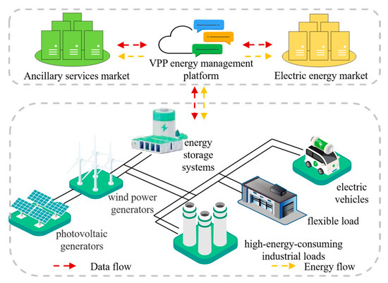
Figure 1.
Energy flow diagram of VPP participating in the ancillary service market.
3. Day-Ahead Phase—Characterization of Internal Resources in VPPs
In the day-ahead phase, the power consumption characteristics of the resources within the VPP are collected and classified according to the degree of flexibility of their units: rigid loads, semi-controlled loads, and controllable loads.
3.1. Rigid Load
A rigid load mainly refers to a base load of electricity consumed by users in the VPP. If the power supply is interrupted, it will cause significant economic losses to the users in the VPP. Therefore, such loads generally cannot be dispatched flexibly and have a certain degree of stability. They must always be active:
where is the power of the rigid load in the VPP at time .
The set of all moments in the dispatch cycle is denoted as , and the power consumed by the rigid load in a dispatch cycle can be calculated as follows:
3.2. Semi-Controlled Load
A semi-controlled load mainly refers to a load in the VPP that exhibits strong randomness and intermittency due to external factors, resulting in a low degree of flexibility in VPP scheduling.
3.2.1. Clean Energy Generation Model
The generation of clean energy, such as wind power and photovoltaics, is affected by geographic and meteorological factors, leading to model uncertainty and random fluctuations in output power, resulting in low predictability and flexibility in scheduling within the VPP. Stochastic optimization methods can address this uncertainty, employing random variables with certain probability distributions. However, these methods suffer from issues such as high computational complexity, the need for more parameters, and long computation times in practical applications. Additionally, in the context of the optimal scheduling of VPPs, the uncertainty of clean energy generation must be incorporated into the scheduling model constraints to account for extreme weather conditions that may occur during power generation. Stochastic optimization methods may not be suitable in this case, as they could result in safety accidents.
Adaptive robust optimization methods aim to address the robustness and adaptability of optimization problems in the presence of uncertainties. This approach combines the concepts of adaptivity and robustness to ensure an effective search for optimal solutions in the face of various uncertain factors. It considers the feasibility and conservatism of solutions under uncertain conditions, at the cost of increased operating expenses, to guarantee the proposed solution’s robust feasibility. Compared to stochastic optimization methods, it requires fewer parameters and only relies on the predicted values of clean energy and their corresponding fluctuation intervals.
Therefore, the adaptive robust optimization method was chosen to model the clean energy generation in this paper. As a result, the clean energy generation model in the day-ahead dispatch phase can be obtained as follows:
where is the actual power of clean energy generation at time ; is the predicted power of clean energy generation at time ; is the fluctuating power of clean energy generation at time ; and are the fluctuating state variables of clean energy generation at time .
This paper introduces the uncertainty budget value in the scheduling cycle to account for the variability in the distribution of wind and solar resources, which can lead to smoother and less volatile aggregated output compared to individual output. This value constrains the uncertainty of the clean energy generation model based on the scheduling period, thus limiting the conservatism of the scheduling results:
Then, the amount of electricity generated by clean energy in a dispatch cycle is:
To improve the robustness of the power space of the clean energy generation model, the maximum value and the minimum value of the power generated by clean energy in the dispatch cycle can be obtained by taking the positive and negative fluctuation state variables as , according to the set budget value of dispatch cycle uncertainty:
3.2.2. Electric Vehicle Load Model
The electric vehicle’s storage battery provides it with flexible power regulation characteristics. Unlike traditional storage batteries, the charging and discharging behavior of electric vehicle users is somewhat random and needs to meet the users’ comfort, thus having a degree of uncertainty. To account for this uncertainty, this paper makes the following assumptions for the electric vehicle charging operation model:
- No specific time limit is set for when the electric vehicle users disconnect from the network;
- To meet user travel requirements and improve user satisfaction, a guaranteed charging power for electric vehicles is set.
Thus, the actual power consumed by the electric vehicle at time is given by:
where is the number of electric vehicles in the VPP; is the power consumed by the electric vehicle at time .
The amount of electricity consumed by the electric vehicle during a dispatch cycle can be obtained as:
To determine the adjustable power range of electric vehicles, we set the maximum number of electric vehicles on the network in the dispatch cycle as and the minimum number as . Based on the settings mentioned above, the power of electric vehicles at time in the dispatch cycle is constrained to be no lower than the charging guaranteed power and no higher than the maximum charging power of electric vehicles. Therefore, we can obtain the upper limit and lower limit of the power consumed by electric vehicles in the dispatch cycle, while taking into account the robustness:
where is the maximum acceptable charging power of the electric vehicle at time ; is the charging guaranteed power of the electric vehicle at time .
3.2.3. High-Energy-Consuming Industrial Loads Model
Based on the characteristics of high-energy-consuming loads, this paper classifies them into discrete adjustable high-energy-consuming loads and continuous adjustable high-energy-consuming loads, which have certain demand response capabilities but low controllability due to their close relationship with product quality. Discrete adjustable high-energy-consuming loads, such as electrolytic aluminum, silicon carbide, and magnesium oxide, have production limitations and cannot participate in grid regulation frequently. On the other hand, continuous adjustable high-energy-consuming loads, such as ferroalloy, have no strict requirement on regulation time and can be continuously regulated within the regulation range. The high-energy-consuming load model is analyzed and established according to the above classification.
- Discrete Adjustable High Energy Consumption Load Model
Based on the characteristics of the discrete adjustable high-energy-consuming load, its regulation capability is lower than that of the continuous type. This is because the load production process has a high demand for electrical energy stability, and it is difficult to respond to the grid adjustment signal frequently. Therefore, the actual power consumption is as follows:
where is the number of discrete adjustable high-energy-consuming loads in the VPP; is the power of discrete adjustable high-energy-consuming loads in the VPP participating in grid regulation at time ; is the power of discrete adjustable high-energy-consuming loads in the VPP scheduled to be consumed before time . is the power consumption of discrete controllable high-energy load within the virtual power plant at time according to the pre-scheduled plan.
Based on the characteristics of the discrete adjustable high-energy-consuming load, this paper defines the decision variables and for the load’s participation in grid regulation at time . The decision variable represents the actual power consumption of the load, and the decision variable represents the participation coefficient of the load in grid regulation. Using these decision variables, the power expression for the discrete adjustable high-energy-consuming load at time can be obtained as follows:
where ; is the maximum regulation of the discrete adjustable high-energy-consuming load in the VPP at time .
In order to not interfere with the normal production of high-energy-consuming enterprises in the VPP, the discrete adjustable high-energy-consuming loads need to meet the following constraints on capacity:
where and are the upper and lower limits of the regulation capacity of the discrete adjustable high-energy-consuming load in the VPP at time .
The discrete adjustable load has certain constraints on the regulation time. After the load participates in grid regulation, it needs to run steadily for a certain period before considering whether to make the following regulation. Additionally, the load must participate in the regulation within the maximum time limit. Thus, its operation time must be constrained as follows:
where and are the minimum stable operation interval and the maximum continuous operation time for the discrete adjustable high-energy-consuming load to participate in grid regulation in the VPP.
As some of the equipment covered by this type of load requires high precision during production and has limited component impact resistance, it cannot be involved in frequent regulation. Therefore, it needs to comply with the regulation number constraints:
where is the maximum number of regulations of the discrete adjustable high-energy-consuming load in a dispatch cycle in a VPP.
The power consumed by the discrete adjustable high-energy-consuming load in a dispatch cycle can be obtained by summing up the power consumed at each time in the dispatch cycle, which is expressed as follows:
Based on the given constraints and considering the boundary situations for discrete adjustable high-energy-consuming loads participating in grid regulation, the minimum stable operation interval time and maximum operation time within a dispatching cycle are determined according to the upper and lower limits of regulation capacity. The participation in the regulation of a cycle is set to the maximum number of regulations . The maximum and minimum values of power consumption and for discrete adjustable high-energy-consuming loads within a dispatching cycle can be obtained as follows:
where is the operating interval time of the discrete adjustable high-energy-consuming load ; is the operating time of the discrete adjustable high-energy-consuming load .
- B.
- Continuous Adjustable High Energy Consumption Load Model
The power stability needs of continuous adjustable loads during regulation are lower compared to discrete adjustable loads, allowing for continuous regulation. The actual power consumption of the continuous adjustable high-energy-consuming load at time can be expressed as:
where is the power of the continuous adjustable high-energy-consuming load in the VPP participating in grid regulation at time ; is the power consumed by the continuous adjustable high-energy-consuming load in the VPP planned before time .
After analyzing the characteristics of continuous adjustable high-energy-consuming loads, this paper set the regulation coefficient for the continuous adjustable high-energy-consuming load participating in grid regulation. Therefore, the expression for the power consumption of the continuous adjustable high-energy-consuming load at time can be obtained as follows:
where is the maximum regulation of the continuous adjustable high-energy-consuming load in the VPP at time .
In industrial-type loads, there is a close relationship between their electricity consumption and the quality of their products. Therefore, constraints on the upper and lower limits of load regulation are necessary for them:
where and are the upper and lower limits of the regulating capacity of the continuous adjustable high-energy-consuming load in the VPP at time .
To further ensure the quality and production safety of their manufactured products, a constraint on the load response rate needs to be considered when continuous adjustable high-energy-consuming loads participate in the grid response:
where and are the upper and lower limits of the fluctuation rate of continuous adjustable high-energy-consuming load .
The power consumed by the continuous adjustable high-energy-consuming load in one dispatching cycle can be obtained as:
Based on the aforementioned constraints, by considering the extreme scenario of a continuous adjustable high-energy-consuming load participating in grid regulation and regulating the load in all periods within the upper and lower limits of regulation during the dispatching cycle, we can determine the maximum power consumption value and the minimum power consumption value of the load in one dispatching cycle, which can be expressed as:
3.3. Controllable Load
A controllable load mainly refers to a load in the VPP that is less affected by external factors and has more control over its power consumption and usage time. Adjusting these loads’ power consumption will not significantly impact the user’s load, allowing the VPP to be dispatched flexibly according to instructions.
3.3.1. Energy Storage Systems Model
The energy storage systems can be charged or discharged at any moment, subject to constraints on the charging and discharging power as well as the energy capacity of the system, which can be expressed as follows:
where and are the charging power and discharging power of the energy storage system at time ; and are the upper limits of the charging and discharging power of the energy storage system at time ; is the storage capacity of the energy storage system at time ; is the maximum storable capacity of the energy storage system .
The energy storage systems’ batteries are not ideal and experience energy loss during charging and discharging. This paper sets the energy loss coefficient of energy storage systems during the charging and discharging process as , with a value range of . Thus, the energy state conversion function can be used to describe the balance between the capacity of energy storage systems and their charging and discharging relationship:
where is the time interval from time to time .
In addition, the energy storage system cannot be in a state of charging and discharging at the same time, and the energy balance of charging and discharging energy in a dispatch cycle needs to be maintained constant, that is:
Then, the power consumed by the energy storage systems during a dispatch cycle is:
where is the number of energy storage systems in the VPP.
From a dispatch cycle perspective, assuming that the energy storage systems operate at the maximum charging power and participate in the auxiliary service market, the maximum power consumption of the energy storage systems can be reached, which can be expressed as:
3.3.2. Flexible Load Model
This paper distinguishes between shiftable loads and curtailable loads in the VPP and establishes separate load models according to their different methods of flexible load regulation.
- Shiftable Load
A shiftable load is a type of load subject to restrictions, such as production processes, and requires adjustments to its overall power consumption curve to meet grid regulation requirements. The timing of these adjustments is often related to the comfort level of the users in the VPP and the compensation policy of the power company. A critical characteristic of shiftable loads is that they must be guaranteed to run uninterrupted until the load is completed once they are started. To more accurately model shiftable loads, this paper introduces a binary operating state variable for the shiftable load at time , as well as binary start and stop state variables and , which are used to construct shiftable load constraints.
The first constraint on the duration of the shiftable load ensures that once it starts operating, it must continue until the task is completed without any interruption:
where and are the earliest start and latest stop times of the shiftable load , and is the total operating time of the shiftable load .
The logical relationship between the operating state and the start/stop state variables of a shiftable load is shown below. When the operating state of the shiftable load changes from 0 to 1 at time , the start state variable of the shiftable load at time is 1:
Then, the power consumed by the shiftable load during a dispatch cycle is:
where is the number of shiftable loads in the VPP; is the power of the shiftable load in the VPP at time .
Assuming that all of the shiftable loads in the VPP participate in the auxiliary service during a dispatch cycle, the maximum power consumption of the shiftable loads during the dispatch cycle can be calculated as follows:
- B.
- Curtailable Load
A curtailable load refers to a load that can be partially or fully curtailed based on the actual supply and demand situation during optimal scheduling. It can be controlled in real time according to the real-time tariff and compensation policy of the power company. The power interval constraint is applied to its model as follows:
where and are the lower and upper limits of the power interval of the curtailable load at time ; is the operating power of the curtailable load at time .
Then, the amount of electricity consumed by the curtailable load in a dispatch cycle is:
where is the number of loads that can be cut in the VPP.
In a dispatching cycle, the operating power of the curtailable load in the VPP is used as the upper and lower limits of the operating power and . This allows for the determination of the maximum power consumption and minimum power consumption of the curtailable load during the dispatching cycle, which can be expressed as follows:
4. Adjustable Power Space Assessment
4.1. VPP Adjustable Energy Space
In summary, during a dispatching cycle, the VPP can adjust the power upward and downward spaces and based on the power output of the internal power-using units in the day-ahead phase, as follows:
where is the power consumption of the VPP in the day-ahead planning from the power market; is the duration of a dispatch cycle.
Then, the adjustable power of the VPP at time t in the dispatch cycle is:
The variables in the dispatching cycle include: , the charging power of the energy storage device at time ; , the discharging power of the energy storage device at time ; , the discrete adjustable high energy-consuming load participating in grid regulation power at time ; , the continuous adjustable high energy-consuming load participating in grid regulation power at time ; , the operating power of the shiftable load at time ; , the operating power of the curtailable load at time ; , the power generated by clean energy at time ; and , the power consumed by the day-ahead planning electric vehicle at time .
4.2. VPP Peaking/Frequency Adjustable Power Space
4.2.1. VPP Peaking/Frequency Regulation Performance Indicators and Ranking Methods
This paper draws upon and summarizes the domestic and international power markets regarding the performance requirements for adjustable load response in the peak and frequency regulation auxiliary service market [27,28]. It further refines and summarizes the capacity of adjustable load participation in the peak and frequency regulation auxiliary service market. Additionally, for the first time, it introduces the response credibility performance index derived from three key aspects: regulation potential, historical credit, and response cost. The paper presents five time-domain response performance indices for each controllable load.
- VPP Peaking Performance Indicators
Comprehensive analysis reveals that domestic peaking services generally encompass two main aspects [29,30]. Firstly, they facilitate peak shaving and valley filling for each generation entity by combining day-ahead units. Secondly, they aim to maintain the power balance by addressing power deviations based on day-ahead planning. Given these circumstances, the peaking service market necessitates the participation of an adjustable load to respond swiftly within a short timeframe and sustain continuous capacity. Consequently, the peaking service market emphasizes the duration and speed of peaking response from bidding resources. To meet the performance requirements of the peaking service market, this paper refines five adjustable load peaking performance indicators, which quantitatively assess the alignment between the controllable load and the performance requirements of the peaking auxiliary service.
- (1)
- Peaking duration
The peaking duration refers to the minimum duration required to maintain the load response in the VPP at the capacity required by the peaking command after the command is issued by the system.
- (2)
- Peaking response speed
The peaking response speed refers to the minimum speed needed to maintain the load response in the VPP at the capacity required by the peaking command after it is issued by the system.
This paper normalizes the response speed to eliminate the influence of the scale and order of magnitude of each index and make the results more comparable across different indices. Specifically, after obtaining the load response speed , it is divided by the maximum value of the corresponding parameter across all loads and converted into a percentage system. The normalized expression is:
- (3)
- Peaking recovery rate
The peaking recovery rate refers to the rate at which the peaking load in the VPP can be restored after the load has finished responding to the market demand for peaking auxiliary services. It is usually measured in units of power per unit of time.
- (4)
- Peaking response credibility
The peak response credibility refers to the probability that the internal resources of a VPP will respond successfully when called upon to participate in dispatch, taking into account possible abnormal conditions due to equipment or other factors. It reflects the confidence level in the ability of the VPP to provide peaking auxiliary services and can be determined through historical data analysis.
- (5)
- Peaking response cost
The peaking response cost refers to the cost associated with the electricity consumption and dispatch required for the internal resources of the VPP to participate in the market demand response of peaking auxiliary services.
The final peaking performance index is calculated as the weighted average of the various peaking performance indicators:
where , , , and represent the weights assigned to the peaking duration, peaking response speed, peaking recovery rate, peaking response credibility, and peaking response cost indices, respectively. These weights can be determined based on historical data and operational experience.
- B.
- VPP Frequency Performance Indicators
Based on the performance requirements of domestic and international power markets for frequency modulation auxiliary services, it is evident that the system frequency response plays a crucial role in regulating the system frequency [31]. Its characteristics can be summarized as follows: it buffers sudden changes in power generation or load power abnormalities, automatically balances the system during fast and small amplitude load fluctuations, and regulates frequency decay with some differences. The frequency modulation auxiliary service market demands fast response speeds and frequent response times. Therefore, it emphasizes the adjustable load’s response speed and frequency. In light of this, this paper defines five adjustable load frequency modulation performance indicators as follows:
- (1)
- Frequency response speed
The frequency response speed is the maximum time taken by the load in a VPP to reach the output level required by the frequency after receiving the frequency command from the system.
- (2)
- Response frequency
The response frequency is the number of times a load in a VPP can respond to a frequency command within a specified period.
- (3)
- Frequency recovery rate
The frequency recovery rate is the amount of frequency response that can be recovered per unit of time after the load in the VPP has completed its response to the frequency command from the system.
- (4)
- Frequency response confidence
The frequency response confidence refers to the probability of a successful response of the frequency load after it participates in the frequency auxiliary service market.
- (5)
- Frequency response cost
The frequency response cost is incurred for the VPP to participate in the frequency auxiliary service market demand response, including the cost of electricity consumption and dispatch.
The final frequency performance index can be obtained as follows:
where , , , and are the corresponding index weights of the frequency response speed, frequency response frequency, frequency recovery rate, frequency response confidence, and frequency response cost, respectively.
Furthermore, to meet the regulatory requirements of the auxiliary service market for load participation, this paper set the lower limit of acceptable regulation duration for the peak regulation auxiliary service market as , the upper limit of an acceptable regulation response rate as , the lower limit of an acceptable regulation recovery rate as , the lower limit of acceptable regulation response credibility as , and the upper limit of acceptable regulation response cost as . Thus, for the load participating in the peaking auxiliary service, the following constraints are applied:
where is the peaking duration of load ; is the peaking response rate of load ; is the peaking recovery rate of load ; is the peaking response credibility of load ; and is the peaking response cost of load .
In the frequency response, the same constraints on the load participating in the frequency auxiliary service are as follows:
where is the frequency response speed of load ; is the frequency response frequency of load ; is the frequency recovery rate of load ; is the frequency response confidence of load ; is the frequency response cost of load .
- C.
- VPP Ranking Method Based on Peak/Frequency Regulation Performance Indicators
To enable adjustable loads with a better fit to participate in the response quickly and with better regulation efficiency, this study employed a performance index evaluation method to classify and aggregate peak/frequency loads. The specific steps are outlined below:
- (1)
- The peak regulation performance index and the frequency regulation performance index for the load are calculated separately;
- (2)
- The VPP ranks the loads in the adjustable space within the VPP in descending order, based on the load’s corresponding peaking performance index and the frequency regulation performance index , and obtains the load’s ranking position for participation in the peaking auxiliary service market and the ranking position for participation in the frequency regulation auxiliary service market;
- (3)
- The load corresponding to the peak and frequency regulation performance indices is analyzed. If it satisfies and meets the peak load constraint, the load will be put into the peak auxiliary service set . If it satisfies and meets the frequency load constraint, the load will be put into the frequency auxiliary service set . If the load’s ranking in the peak auxiliary service market is equal to the load’s ranking in the frequency auxiliary service market, i.e., , and if the load satisfies the peak load constraint, it will be put into set , and if it satisfies the frequency load constraint, it will be put into set . If it satisfies both the peak and frequency load constraints, the load in the top 50% of the rankings will be put into set , and the load in the bottom 50% will be put into set .
4.2.2. VPP Peaking/Frequency Adjustable Power Space Model
According to the previous description of the internal power consumption unit of the VPP and the peaking auxiliary service set , it is divided into the maximum and minimum load sets and for clean energy and curtailable loads participating in the peaking auxiliary service and the maximum and minimum load sets and for other semi-controlled and controllable types of loads participating in the peaking auxiliary service, and the upward and downward space for the power of the VPP participating in the peaking auxiliary service can be obtained:
where is the power of load at time in the minimum load set of clean energy or curtailable load participating in the peak regulation auxiliary service; is the power of load at time in the maximum load set of other semi-controlled and controllable loads participating in the peak regulation auxiliary service; is the power of load at time in the maximum load set of clean energy or curtailable load participating in the peak regulation auxiliary service; is the power of load at time in the minimum load set of other semi-controlled and controllable loads participating in the peak regulation auxiliary service.
Then, the maximum dispatchable power of the VPP participating in the peaking auxiliary service at time t in the dispatch cycle is:
where is the power of load in the largest load set participating in the peaking auxiliary service at time .
The maximum dispatchable power of the VPP participating in the frequency auxiliary service at time during the dispatch cycle is:
where is the power of load in the largest load set participating in the frequency auxiliary service at time .
5. Real-Time Phase—Optimized Energy Management Regulation Method for VPPs Participating in Auxiliary Service Markets
5.1. Optimal Energy Management Regulation Model for VPP Participation in Auxiliary Service Markets
This section presents the energy management model of VPPs that participate in the ancillary service market based on the previous model. The real-time optimization objective is to minimize the net operating cost of the VPP after participating in the ancillary service market, which is the cost of the power purchased and the adjustable load call cost minus the ancillary service market revenue. The model can be formulated as follows:
where is the cost of the electricity purchased by the VPP from the electricity energy market during a dispatch cycle; is the revenue gained by the VPP from participating in the ancillary service market during a dispatch cycle; is the cost of the VPP’s call to the regulable load during a dispatch cycle; and is the penalty cost incurred by the VPP for failing to meet the established target of the ancillary service market during a dispatch cycle.
5.1.1. Cost of Electricity Purchase
Based on the electricity consumption plan received by the VPP from the electricity energy market before the day in the dispatch cycle and the electricity price information fed back to the VPP by the market in the same cycle, the cost of electricity purchased by the VPP can be calculated as follows:
5.1.2. Participation in Ancillary Service Market Revenue
In real-time operation, the ancillary service market sends the VPP the peaking auxiliary service power and the frequency auxiliary service power , which need to be responded to at each moment. The VPP then needs to allocate and adjust the power consumption for its internal resources in real time to meet the energy consumption needs of these resources and the market’s peaking and frequency regulation needs.
At this stage, the VPP considers the constraint on the adjustable load power and strives to respond to the auxiliary service market while ensuring the resource demand. The VPP can only provide the maximum dispatchable power if the demand cannot be met. Consequently, the peaking auxiliary service power and frequency auxiliary service power that the VPP responds to at time can be obtained, and their adjustment direction is determined by the direction of the peaking auxiliary service power that needs to be responded to, i.e.,:
Then, the power for the VPP participating in the peaking auxiliary service market and the power for the frequency auxiliary service market in a dispatch cycle can be expressed as follows:
In real-time operation, a VPP’s revenue from participation in the ancillary service market during a dispatch cycle is comprised of two components: revenue from participation in the peaking ancillary service market and revenue from participation in the frequency ancillary service market, which can be denoted as and :
- A.
- Participation in peaking auxiliary service market revenue
This paper models the participation of a VPP’s revenue from the peaking auxiliary service market in a dispatch cycle into two parts: grid subsidy revenue and policy subsidy revenue :
The grid subsidy benefits is:
where is the compensation amount per unit of peaking power in a dispatch cycle; is the coefficient representing the proportion of grid upgrade costs delayed due to the VPP’s participation in peaking; is the expansion cost required to upgrade the grid per unit of load; is the maximum load of the baseline load curve of the VPP in a dispatch cycle; and is the maximum load of the load curve of the VPP after participating in peaking in a dispatch cycle.
The policy subsidy benefit is:
where is the amount of subsidy per unit of peaking power of a VPP in a dispatching cycle.
- B.
- Participation in frequency auxiliary service market revenue
The revenue earned by a VPP by participating in the frequency ancillary service market during a dispatch cycle is obtained by summing up the frequency capacity cost and frequency mileage cost of its participation [32], which can be expressed as follows:
where is the frequency capacity cost of the VPP in one dispatch cycle; is the frequency mileage cost of the VPP in one dispatch cycle.
The frequency capacity cost is:
where is the price per unit of frequency capacity in a dispatching cycle; is the reported frequency capacity of a VPP in a dispatching cycle;
The frequency mileage cost is:
where is the price per frequency mile in a dispatch cycle; is the climbing mile in a dispatch cycle.
5.1.3. Invocation Cost
This paper considers the VPP invocation cost, which is composed of several components, including the energy storage system invocation cost , the flexible load invocation cost , the clean energy generation cost , the high-energy-consuming industrial load invocation cost , and the electric vehicle invocation cost :
The cost of the energy storage system is:
where is the depreciation and maintenance cost per unit of power of the energy storage system; is the price of invoking a unit of power of the energy storage system in a dispatch cycle.
The cost of the flexible load is:
where is the cost price of invoking a unit of power to the shiftable load in a dispatch cycle; is the cost price of invoking a unit of power to the curtailable load in a dispatch cycle.
The cost of clean energy generation is:
where is the cost of invoking units of wind power and photovoltaic units in a dispatching cycle.
The cost of the high-energy-consuming industrial load is:
where is the cost price of invoking a unit of power of a discrete adjustable high-energy-consuming load in a dispatch cycle; is the cost price of invoking a unit of power of a continuous adjustable high-energy-consuming load in a dispatch cycle.
The cost of the electric vehicle is:
where is the cost of invoking a unit of power of an electric vehicle in a dispatch cycle.
5.1.4. Penalty Cost
Due to the uncertainty and randomness of the resources in the VPP, there may be a certain deviation between the power of the real-time response of the VPP and the power that the grid needs to respond to, resulting in a certain penalty cost. Therefore, this paper introduces a penalty factor , which is determined based on the minimum accuracy ratio and the actual accuracy ratio Q that can be achieved through the participation of the VPPs in the auxiliary service market, as specified by the grid. The penalty costs are calculated as follows:
where is the ratio of the actual response power of the VPP to the demand response power; is the unit of power penalty cost of the VPP participating in the auxiliary service market during a penalty cycle.
5.2. Optimal Energy Management Regulation Constraints for VPP Participation in Ancillary Service Markets
This paper considers several constraints, including the fundamental power balance constraint, operation constraints for each resource, and interaction constraints with the grid.
5.2.1. Power Balance Constraint
In real-time dispatch, the total power consumption of a VPP during a dispatch cycle satisfies the following constraint:
5.2.2. Operational Constraints for Resource
The internal unit output constraints of the VPP, as analyzed in Section 2, include the following: the rigid load constraint (1), the semi-controlled load constraints (4)–(6), (16)–(19), (25)–(26), and the controllable load constraints (30)–(35), (38)–(43), and (46).
5.2.3. Interaction Constraints with the Grid
The analysis in Chapter 3 indicates that the interaction constraints between the VPP and the grid can be divided into two categories. The first category includes constraints related to the VPP’s participation in electricity energy market transactions, and the second category includes load constraints related to the VPP’s participation in the ancillary service market.
VPPs are required to meet the maximum purchased power limit when purchasing power from the electricity energy market:
where is the maximum purchasable power of the VPP.
Among them, the load constraint for the VPP internal load’s participation in the auxiliary service market consists of (7)–(16). According to the relevant regulations of the electricity market, VPPs are subject to access minimums when participating in the auxiliary service market, and the following requirements constrain their access conditions:
where and are the minimum values of access at time for VPPs participating in the peaking and frequency auxiliary service market, as specified in the electricity market.
The internal resources of the VPP are subject to the following constraints when participating in both the peaking and frequency auxiliary service markets simultaneously:
where and are the actual output values of the VPP’s internal resource participating in the peaking and frequency auxiliary service market at time ; is the adjustable output value of the VPP participating in the auxiliary service market at time .
6. Case Study
This paper uses a VPP as an example to demonstrate the effectiveness of the proposed optimization model for participating in the electricity market. The VPP consists of various resources, including wind turbines, PV turbines (with the corresponding wind power and PV forecast values and fluctuation intervals shown in Figure A1 in Appendix A), EV charging stations (800 charging piles with a maximum charging power of 7 and a guaranteed charging power of 3 ), high energy consumption loads (with the regulation parameters shown in Table A1), energy storage devices (with a maximum charging and discharging power of 10 KW, maximum energy storage power of 100 , and energy loss coefficient of 0.8), and flexible loads (with the parameters of the shiftable load and curtailable load shown in Table A2 and Table A3). The electricity market adopts a time-of-use electricity pricing format. The corresponding electricity price information can be found in Table A4, and the resource parameters within the VPP can be found in Table A5. The VPP purchases power before the day and reports the dispatch interval, responding to real-time power adjustment signals from the market during operation to improve participation in grid regulation and optimize resource allocation and utilization. The market price adjustment signals used in this study were from PJM, U.S.A. The model proposed in this paper was solved using MATLAB’s CPLEX solver. The scheduling period was 24 h (with the simulation steps defined as 1 h), and the maximum number of iterations was set to 300. The processor of the computer was Intel(R) Core(TM) i5-10210U CPU at 1.60 GHz–2.11 GHz, and the RAM was 8 G. The built-in interior-point method was used for solving. The solving process is illustrated in Figure 2.
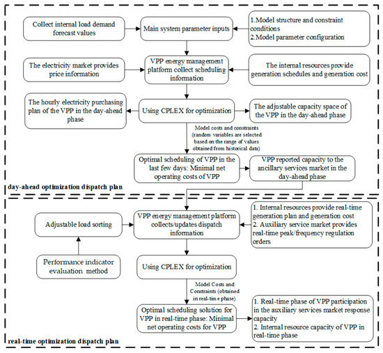
Figure 2.
Flowchart for optimal energy management model of VPP.
6.1. Analysis of the Impact of Clean Energy Uncertainty on the Operation of VPP
To further investigate the impact of uncertainty on the economic feasibility of VPPs, this study computed the costs and benefits associated with VPPs’ participation in the ancillary service market under varying levels of uncertainty in clean energy generation. The curves in the graph correspond to the left y-axis and show the variations in the operational and penalty costs generated by the wind and solar photovoltaic generation models within a scheduling period, considering their uncertainty budgets in the range of 0–24.
As can be seen in Figure 3, with the increase in the uncertainty budget value, the operating cost of clean energy within the VPP shows a trend of first decreasing and then increasing. This is because, with the increase in the uncertainty budget value, the uncertainty of clean energy output also increased. A portion of the clean energy output can participate in the auxiliary service market to generate revenue. However, due to the uncertainty in its output, the actual response penalty cost increased with the increase in the uncertainty budget. The operating cost of wind and PV generating units was minimized when the uncertainty budget of the dispatching cycle and the uncertainty budget of the dispatching cycle were represented by and , respectively.
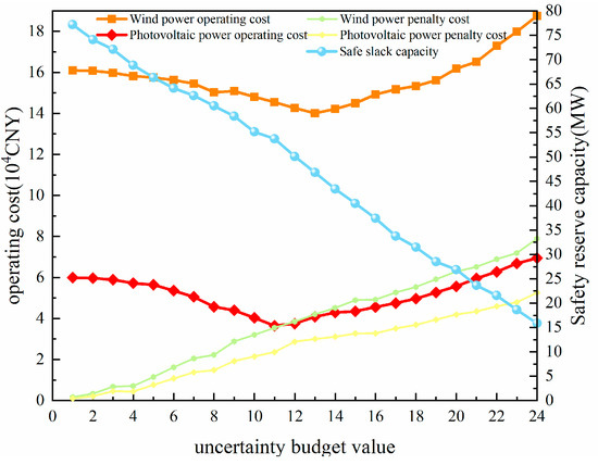
Figure 3.
Impact of uncertainty budget value on scheduling.
Considering the impact of uncertainty on the safety of the VPP, this paper introduces the concept of “safety reserve capacity”, which is defined as the maximum reserve capacity of the VPP that allows for safe operation as uncertainty increases. This measure is used to evaluate the safety of the VPP. To avoid the occasional nature of single-experiment results, 40 simulation runs were performed in the case study of this paper, and the average values were obtained. The resulting curves correspond to the right y-axis, as shown in Figure 3.
It can be observed that when the uncertainty budget value was small, the safety reserve capacity was large, indicating a high level of safety in VPP operation. However, as the uncertainty budget value increased, the safety reserve capacity of the VPP decreased, leading to a decrease in operational reliability. When the uncertainty budget value was set to , the safety reserve capacity of the VPP was 15.867 MW, which was only 20.56% of the safety reserve capacity when the uncertainty budget value was . In this case, the VPP operated under extremely unsafe conditions, facing significant safety risks.
Therefore, in practical operation, it is necessary to select a reasonable value for the uncertainty budget to ensure a certain level of economic efficiency and safety.
Based on the analysis of the results in the figure, the uncertainty budget values for the scheduling period in the wind power and solar photovoltaic generation models are denoted as and . Using these values, an analysis was conducted on the day-ahead to real-time VPP optimization scheduling model proposed in this paper.
6.2. Analysis of Optimal Energy Management Regulation Model Results of VPPs in the Day-Ahead Phase
This section analyzes the scheduling scheme of VPPs participating in the auxiliary service market at the day-ahead phase.
Figure 4 shows the composition of the adjustable capacity space for the VPP in the day-ahead stage. Analyzing the results in Figure 4, it can be observed that high-energy loads accounted for 25.36% to 45.08% of the adjustable capacity space within one scheduling period, which is significantly higher than the proportions of the other semi-controllable and controllable loads within the VPP. Compared to other adjustable loads, it can be inferred that high-energy industrial users with sufficient storage capacity can provide frequent and short interruptions without adverse effects on their production. Furthermore, compared to the other adjustable loads, the curtailable load in the adjustable capacity space exhibited relatively stable output, with fluctuation ranging from −12.84% to +10.62% and from −7.41% to +10.28%, respectively. Therefore, in comparison to other controllable loads, curtailable load participation can provide more stable output.
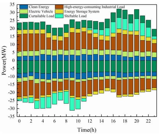
Figure 4.
VPP adjustable power space.
Figure 5 displays the reported capacity and the power purchased from the energy market by the VPP. The blue line in Figure 5, corresponding to the right scale, represents the electric power purchased by the VPP from the energy market. It can be observed that the maximum power purchase by the VPP occurred at 4:00 during off-peak hours, influenced by the “peak and valley tariffs” factor. Analyzing the histogram in Figure 5 reveals that the reported capacity of the VPP prior to the day aligned with the adjustable power space but was slightly lower. The extent of this discrepancy is related to the electricity price during the corresponding period. Taking the adjustable space as an example, during off-peak hours, the reported capacity of the VPP decreased by an average of 1.98 MW compared to the adjustable power space. Similarly, during normal hours and peak hours, the reported capacity decreased by averages of 2.7 MW and 3.21 MW, respectively, compared to the adjustable power space. This reduction in reported capacity was due to the inherent uncertainty of the covered resources. On the one hand, reducing the reported capacity provided a certain amount of load reserve for internal operations, particularly during high-demand peak electricity price periods caused by abnormal working conditions. On the other hand, it helped mitigate the risk and associated costs arising from an insufficient actual adjustable capacity.
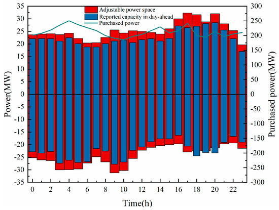
Figure 5.
Capacity and power purchases reported by VPPs in the day-ahead phase.
6.3. Analysis of the Impact of Performance Indicator Evaluation Methods on Adjustable Load
In order to compare the impact of the proposed performance indicator evaluation method on the optimization results, this paper analyzes three scenarios: (1) not using the performance index evaluation method, (2) using the average-weighted performance index evaluation method (, ), and (3) using the performance index evaluation method with weights obtained from historical experience data (, , , , , , , , , ). Through simulations, these three evaluation methods were compared in terms of their impact on the VPP’s participation in the auxiliary service market. The maximum fluctuation deviation of semi-controlled resources was determined based on historical forecast deviations. This paper set the uncertainty budget values for clean energy dispatch cycles as and (due to the consideration of the optimized scheduling structure of the aggregated VPP, the spatial scale’s influence on uncertainty was ignored). Table 1 presents the electricity generation cost, auxiliary service market revenue, and the total cost incurred by the VPP when participating in the auxiliary service market.

Table 1.
Electricity cost and benefit.
The results in Table 1 demonstrate that both cases that used the performance indicator assessment method decreased the cost of electricity generation and increased the revenue of the VPP participating in the ancillary service market, leading to a substantial decrease in the VPP’s total operating cost, and thereby highlighting the usefulness of the performance indicator assessment method. Furthermore, the choice of weightings in the indicator evaluation method can impact the total cost of the VPP due to the varying performance requirements of the resources that participated in different ancillary service markets. For instance, the peaking ancillary service market placed a greater emphasis on the response time and response speed of the participating loads, while the frequency ancillary service market prioritized the response speed and response frequency of the loads. The subsequent analysis delves into the real-time dispatch outcomes of the performance indicator assessment method that acquired weights through historical empirical data.
6.4. Analysis of Optimal Energy Management Regulation Model Results in the Real-Time Phase
This section analyzes the real-time scheduling results of the VPP participating in the ancillary service market based on the model proposed in this paper. In this section, the actual response and optimized scheduling results of the VPP during the pre-real-time stage were calculated based on the uncertainties and of clean energy. The performance indicators for sorting the loads within the VPP were evaluated using a weighted evaluation method based on historical empirical data.
Figure 6 illustrates the actual response capacity of the VPP when receiving instructions for peak shaving and peak regulation from the auxiliary service market. This graph compares the VPP’s actual response capacity with the adjustable space and reported capacity in the day-ahead stage within the same dispatch cycle during the day-ahead to real-time two-phase process. The actual response capacity of the VPP was determined by considering the actual peak shaving and frequency regulation signal instructions received from the ancillary service market. Appendix A Figure A2 provides a comparison of the peak shaving and frequency regulation signal instructions between the day-ahead and actual scenarios.
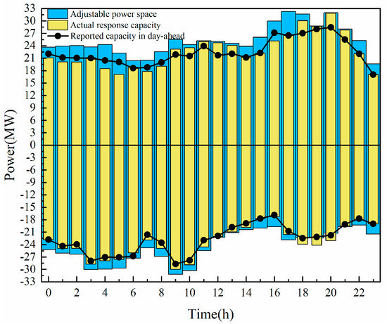
Figure 6.
Actual response capacity of the VPP.
In Figure 6, it can be observed that the difference between the actual response capacity of the virtual power plant and the average reported upper and lower capacities were 1.152 MW and 0.98 MW, respectively. The differences between the actual response capacity of the virtual power plant and the average adjustable capacity space were 2.534 MW and 1.328 MW, respectively. The actual response capacity of the VPP was generally consistent with the reported capacity in the day-ahead stage, and it was closer to the reported capacity compared to the adjustable capacity space in the real-time stage of the VPP. This also demonstrates the effectiveness of the day-ahead optimization scheduling. However, there were certain deviations between the actual capacity and the reported capacity in some periods. For example, at period 4:00–5:00, the upward capacity of the VPP participating in the ancillary service market decreased. By analyzing real-time peak shaving and frequency regulation signals in Figure A2, it can be observed that this was due to a reduction in the actual upward peak shaving and frequency regulation signals required by the ancillary service market compared to the day-ahead stage. In order to improve the economic efficiency of the VPP and reduce the cost of load activation, the actual upward capacity of the VPP was reduced compared to the day-ahead stage.
On the other hand, during 18:00–20:00, the actual response capacity exceeded the capacity reported by the VPP in the day-ahead stage. According to the analysis of Figure A2, this was because, at these moments, the uncertainty in the adjustment signals resulted in a significant increase in the resources required by the ancillary service market compared to the day-ahead period. The actual upward and downward signal deviations from the day-ahead average reached 0.9639 MW and −1.2125 MW, respectively. Due to the penalty coefficient factor being dependent on accuracy, the VPP faced substantial penalty costs. Upon evaluation, it was realized that the VPP could reduce the load reserve and provide more capacity to the ancillary service market, significantly reducing the penalty costs. However, this approach also introduced certain operational risks.
From the above analysis, it can be concluded that the uncertainty in the adjustment signals had a significant impact on the actual response of the VPP. This also confirms the importance of considering the uncertainty of peak shaving and frequency regulation in the real-time stage of the ancillary service market.
Figure 7 illustrates the actual participation of the VPP in the peak shaving and frequency regulation capacities. It can be observed that the VPP’s controllable load had a higher proportion of participation in the frequency regulation market during periods of low electricity demand, while it had a higher proportion of participation in the peak shaving market during periods of high electricity demand. The real-time compensation prices within the scheduling period also influenced this. For instance, the VPP exhibited higher peak shaving output during 11:00–14:00 and 18:00–20:00, which coincided with the peak electricity demand periods. This is because the auxiliary service market offered relatively higher peak shaving prices during these periods. From an economic perspective, the VPP strategically reallocated a portion of its load from the frequency regulation market to the peak shaving market in order to maximize its economic benefits while meeting the demand for peak shaving.
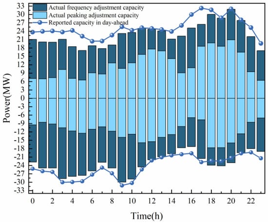
Figure 7.
Actual peaking and frequency adjustment capacity.
To further validate the effectiveness of the proposed optimization scheduling methods in this study, we conducted optimization and scheduling analysis by comparing the methods proposed in this paper with those presented in references [33,34,35]. In Case 1, the day-ahead to real-time stage VPP optimization scheduling method proposed in this paper was employed. In Case 2, the day-ahead to real-time stage VPP optimization scheduling method was used, where the adjustable capacity of the VPP in the day-ahead stage was set equal to the reported capacity.
Case 3 considered the uncertainties in the electricity price, wind power output, and demand response, resulting in the optimization scheduling results for the day-ahead stage without considering the real-time stage impact. Case 4 focused only on the intra-day stage, optimizing and coordinating the demand-side load and energy storage units, such as battery systems, based on the real-time electricity price mechanism and aiming for the optimal economic benefits of each resource. However, it did not consider the day-ahead capacity and load performance limitations. Case 5 considered the day-ahead to the real-time stage, where the electricity exchange with the power market was determined in the day-ahead stage, and in the real-time stage, the dispatchable units and energy storage were allocated based on the fluctuation of the stochastic generating units. However, it did not consider the evaluation of adjustable loads and variations in the real-time adjustment signals. The optimization scheduling results for these different methods are presented in the following figure.
In Figure 8, it can be observed that compared to the optimization scheduling schemes in references [33,34], which considered only the day-ahead or real-time stages, the proposed optimization scheduling scheme in this paper led to increased revenue in the ancillary service market and a significant decrease in total costs, resulting in a significant increase in net operating costs. In the case of reference [35], Case 5 considered optimization scheduling in both the day-ahead and real-time stages. It showed an increase in total costs by CNY 24.4894 compared to Case 2, and a decrease in revenue from participating in ancillary services by CNY 37.517 . The final net operating cost was CNY 300.6398 , close to the net operating cost of CNY 307.294 when the performance evaluation method was not used, as discussed in Section 6.3. This suggests that one reason for the increase in the net operating costs was the failure to consider the impact of VPP participation in the peak shaving and frequency regulation performance indicators. By comparing Case 1 and Case 2, it was found that the revenue from participating in the auxiliary service market in Case 1 was decreased by CNY 7.7691 compared to Case 2. However, the cost was reduced by CNY 23.4165 , indicating a decrease in the net operating cost. This also demonstrates that the proposed optimization method in this paper considered abnormal conditions in the operation of the VPP and exhibited a certain level of conservatism.
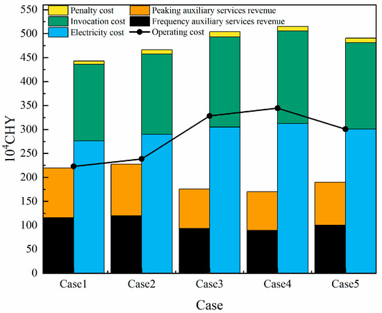
Figure 8.
Resource output factor within the VPP. Comparative analysis under different circumstances.
Figure 9 depicts the actual output of the VPP’s resources in peak shaving and frequency regulation. It can be observed that during the early morning and afternoon periods, the participation of the VPP’s resources in the peak shaving capacity was relatively low. One of the reasons is that the income from participating in the peak shaving auxiliary services was lower during these periods. The primary sources of regulation capacity during these periods were high-energy-consuming loads and adjustable loads, while clean energy sources, energy storage, and electric vehicles contributed to a smaller portion of the peak shaving capacity. For example, the cost of utilizing energy storage was CNY 0.24 , while the depreciation and maintenance cost was CNY 0.02 . During the early morning and afternoon periods, the income from participating in the peak shaving auxiliary services was lower than the cost of utilizing energy storage, resulting in the energy storage system operating at its minimum output level and generating negative profits.
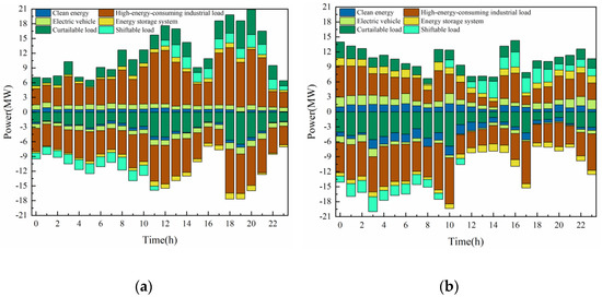
Figure 9.
Resource output factor within the VPP. (a) Actual peaking regulation output of VPP. (b) Actual frequency regulation output of VPP.
The graph shows that the main sources of frequency regulation auxiliary services were high-energy-consuming loads, adjustable loads, and transferable loads. Compared to the peaking auxiliary service market, the energy storage system provided a larger adjustable capacity to the frequency auxiliary service market. This is mainly because the price in the frequency auxiliary service market was higher than the energy storage system’s cost. Additionally, the energy storage system exhibited excellent response capabilities, significantly increasing its output level for frequency regulation.
The following analysis is dedicated to examining the high-energy-consuming loads that exhibited the highest power output within the VPP. The aim was to delve deeper into the influence of load flexibility on the optimization scheduling of the VPP. To establish a control group, two scenarios were compared: Scenario 1 incorporated the flexibility of high-energy-consuming loads, while Scenario 2 disregarded their flexibility. Optimization scheduling analyses were conducted for both scenarios.
Upon comparing the findings presented in Figure 10, it is evident that Scenario 2 corresponds to optimization scheduling without considering the flexibility of high-energy-consuming loads. In situations where the required regulation capacity is low, Scenario 2 compensates by increasing the output of other resources to meet the regulation needs, resulting in comparable resource output values to Scenario 1. In Scenario 2, the up-regulation output in the peaking ancillary service market experiences a reduction of 24.1% compared to Scenario 1, whereas the up-regulation output in the frequency ancillary service market decreases by 19.93%. This indicates a greater inclination towards participating in the frequency ancillary service market, as it offers higher profitability and attracts adjustable loads with higher activation costs, such as energy storage, thereby significantly increasing their output. However, this increase in participation also leads to higher invocation costs. During periods with high demand for regulation capacity in the peaking ancillary service market, Scenario 2 exhibits more substantial differences in output compared to Scenario 1. Despite the higher compensation price for peaking during these periods, the VPP cannot contribute additional adjustable loads to the peaking ancillary service market, as depicted in Figure 10a from 18–21 h.
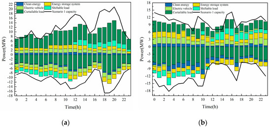
Figure 10.
Actual peak shaving and frequency regulation output of the VPP without considering high-energy-consuming loads. (a) Actual peaking regulation output of VPP. (b) Actual frequency regulation output of VPP.
Table 2 illustrates the numerical analysis of how high-energy-consuming load flexibility affected the optimization scheduling strategy and revenue of the VPP. The results show that integrating the flexibility of high-energy-consuming loads into the optimization scheduling model allowed for a greater adjustment capacity, leading to increased participation in the ancillary service market and reduced net operating costs for the VPP. This demonstrates the effectiveness of incorporating high-energy-consuming loads in ancillary service regulation, as it enhanced power system flexibility and generated profits.
Table 2.
Impact of high-energy-consuming loads on optimization scheduling results.
To examine the effects of actual peak shaving, frequency regulation signals, and other factors on the optimization scheduling results in practical operation, this study introduced the resource output factor as an evaluation indicator. The resource output factor is defined as the ratio of the actual response capacity in resource optimization scheduling to the reported capacity in the day-ahead stage. A comparative analysis was conducted on the reported and actual output capacities of each resource. The resource output factors for different resources are shown in Figure 11.
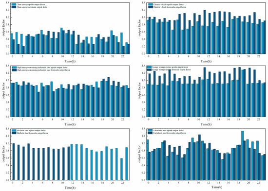
Figure 11.
Resource output factor within the VPP.
It can be observed that in the actual operation of the VPP, clean energy resources exhibited higher fluctuations compared to the other adjustable loads. The average values of the resource output factors for up-regulation and down-regulation were 0.48812 and 0.45381, respectively. This is due to the inherent volatility and instability of clean energy resources. After evaluating the indicators using the indicator evaluation method, their rankings were relatively lower. Consequently, their participation in the capacity of the ancillary service market decreased compared to the day-ahead stage.
Compared to other resources, high-consumption loads and shiftable loads exhibited relatively stable output values. The average values of the upward and downward resource output factors for high-consumption loads were 0.87395 and 0.89417, respectively, indicating that their actual output was generally consistent with the reported capacity. This indirectly suggests the potential for the adjustment of high-consumption loads. The graph shows instances where the resource output factor for electric vehicles exceeds 1. This indicates that electric vehicles had a relatively higher ranking in load prioritization. Additionally, this can be attributed to the conservative nature of the adjustable capacity model used for evaluating electric vehicles in this study. The actual adjustable capacity of electric vehicles was greater than the evaluated value. For the energy storage devices shown in the graph, there were cases where the upward output exceeded the reported capacity. This implies that the energy storage devices can respond quickly and participate in auxiliary service market regulation more effectively compared to other loads during actual operation.
7. Conclusions
A method that considers industrial loads by combining the day-ahead and real-time stages was proposed in this paper to evaluate the adjustable power space of VPPs, and an optimal dispatching model was also proposed. The following conclusions have been drawn from the analysis of the mathematical simulation:
- The uncertainty of clean energy generation can impact the operational efficiency of VPPs. The analysis of its operating costs revealed that clean energy participation in the ancillary service market necessitated a reasonable value for the uncertainty budget to ensure a balance between economic profitability and security.
- The high-energy-consuming industrial load capacity had a stronger power output stability compared to the other flexibility resources, and its adjustable capacity was significant. As a flexible resource participating in the auxiliary service market, it can not only enhance the flexibility of the power system but also generate a certain amount of profit.
- The real-time scheduling of VPPs based on the index performance evaluation method proposed in this paper can effectively reduce the total cost of VPPs, improve the stability of their participation in the auxiliary service market, and enhance the economic benefits of VPP operations.
However, we are also aware of the limitations of our approach in this study. The industrial load model and resource constraint assumptions considered in this paper may not fully cover various real-world situations. Future research can further explore more complex load models and resource constraints to improve the accuracy and applicability of the model. Additionally, studying the uncertainty of electric vehicles is also an important direction to better address their impact on the operation of virtual power plants. Furthermore, in the data-processing process, this paper may have overlooked the potential impacts and risks brought by certain uncertain factors. In our future research, we will incorporate more uncertainty analysis methods to enhance the reliability and applicability of our research results.
In summary, this study provides an effective approach to the optimization energy management of VPPs participating in the ancillary service market and serves as a reference and inspiration for future related research. We hope that the findings of this paper will contribute to the development of sustainable energy systems and the construction of smart grids.
Author Contributions
Conceptualization, Y.W.; methodology, Y.W. and G.L.; software, Y.W.; validation, Y.W., H.M. and Z.L.; formal analysis, Y.W.; investigation, G.L., H.M. and Z.L.; resources, B.Z.; data curation, B.Z.; writing—original draft preparation, Y.W. and G.L.; writing—review and editing, G.L. and B.Z.; visualization, G.L. and H.M.; supervision, G.L. and B.Z.; project administration, B.Z.; funding acquisition, G.L. All authors have read and agreed to the published version of the manuscript.
Funding
This work was supported in part by the National Natural Science Foundation of China—Self-organizing Aggregation and Regulation Theory of Massive Resources Virtual Power Plant for Power Grid Balance Demand (Grant No. U22B20115), in part by the Guangdong Basic and Applied Basic Research Foundation (Grant No. 2021A1515110778), and in part by the Science and Technology Projects of Liaoning Province (Grant No. 2022-MS-110).
Institutional Review Board Statement
Not applicable.
Informed Consent Statement
Not applicable.
Data Availability Statement
Not applicable.
Conflicts of Interest
The authors declare no conflict of interest.
Appendix A
Table A1.
VPP participation in high-energy-consuming load regulation parameters.
Table A1.
VPP participation in high-energy-consuming load regulation parameters.
| High-Energy-Consuming Load | Discrete Adjustable High-Energy-Consumption Load | Continuous Adjustable High-Energy-Consumption Load | |||
|---|---|---|---|---|---|
| Electrolytic Aluminum Plant | Electrofusion Magnesium Plant | Silicon Carbide Plant | Ferroalloy Plant 1 | Ferroalloy Plant 2 | |
| Rated capacity (MW) | 70 | 20 | 24 | 16.5 | 55 |
| Maximum upward adjustment capacity (MW) | 7.7 | 1.6 | 3.6 | 2.1 | 3.4 |
| Maximum down-regulation capacity (MW) | 3 | 1.7 | 4.2 | 1.6 | 3.8 |
| Maximum rate of load increase (MW/15 min) | - | - | - | 0.9 | 1 |
| Maximum rate of load shedding (MW/15 min) | - | - | - | 0.6 | 2.1 |
| Minimum interval time (h) | 3 | 2 | 2 | - | - |
| Maximum continuous running time (h) | 5 | 4 | 6.5 | - | - |
| Maximum number of adjustments (h) | 3 | 4 | 3 | - | - |
Table A2.
VPP curtailable load parameters.
Table A2.
VPP curtailable load parameters.
| Load Subsequence | |||||
|---|---|---|---|---|---|
| 1 | 0.8 | 9 | 22 | 5 | [13,17] |
| 2 | 4.2 | 14 | 22 | 3 | [19,21] |
| 3 | 1.37 | 7 | 20 | 8 | [12,19] |
| 4 | 2.04 | 9 | 24 | 6 | [15,20] |
| 5 | 1.6 | 11 | 24 | 5 | [14,18] |
| 6 | 1.86 | 12 | 24 | 3 | [20,22] |
| 7 | 1.2 | 6 | 18 | 7 | [11,17] |
Table A3.
VPP shiftable load parameters.
Table A3.
VPP shiftable load parameters.
| Load Subsequence | Load Subsequence | ||||
|---|---|---|---|---|---|
| 1 | 0.36 | 0.61 | 6 | 1.28 | 1.92 |
| 2 | 0.13 | 0.75 | 7 | 0.29 | 0.57 |
| 3 | 0.55 | 0.96 | 8 | 0.31 | 0.64 |
| 4 | 0.27 | 0.52 | 9 | 0.25 | 0.68 |
| 5 | 0.42 | 0.64 | 10 | 0.54 | 0.89 |
Table A4.
Electricity energy market purchase price.
Table A4.
Electricity energy market purchase price.
| Time | Operation Status | |
|---|---|---|
| 00:00–08:00 | Low load period | 0.03139 |
| 08:00–15:00, 17:00–22:00 | Peak load period | 0.09231 |
| 15:00–17:00, 22:00–24:00 | Medium load period | 0.06208 |
Table A5.
VPP internal resource parameters.
Table A5.
VPP internal resource parameters.
| Parameters | |
|---|---|
| 0.002 | |
| 0.024 | |
| 0.021 | |
| 0.012 | |
| 0.018 | |
| 0.025 | |
| 0.012 | |
| 0.008 | |
| 0.0284 |

Figure A1.
Wind power and photovoltaic forecasts and their fluctuation intervals.

Figure A2.
Comparison of peak shaving and frequency regulation signals between day-ahead and real-time scenarios. (a) Comparison of peak shaving signals. (b) Comparison of frequency regulation signals.
References
- Liu, S.; Lin, Z.; Jiang, Y.; Zhang, T.; Yang, L.; Tan, W.; Lu, F. Modelling and Discussion on Emission Reduction Transformation Path of China’s Electric Power Industry under “Double Carbon” Goal. Heliyon 2022, 8, e10497. [Google Scholar] [CrossRef]
- Fateh, D.; Eldoromi, M.; Moti Birjandi, A.A. Uncertainty Modeling of Renewable Energy Sources. In Scheduling and Operation of Virtual Power Plants; Elsevier: Amsterdam, The Netherlands, 2022; pp. 193–208. [Google Scholar]
- do Prado, J.C.; Qiao, W. A Stochastic Decision-Making Model for an Electricity Retailer with Intermittent Renewable Energy and Short-Term Demand Response. IEEE Trans. Smart Grid 2019, 10, 2581–2592. [Google Scholar] [CrossRef]
- Villar, J.; Bessa, R.; Matos, M. Flexibility Products and Markets: Literature Review. Electr. Power Syst. Res. 2018, 154, 329–340. [Google Scholar] [CrossRef]
- Jiang, T.; Chung, C.Y.; Ju, P.; Gong, Y. A Multi-Timescale Allocation Algorithm of Energy and Power for Demand Response in Smart Grids: A Stackelberg Game Approach. IEEE Trans. Sustain. Energy 2022, 13, 1580–1593. [Google Scholar] [CrossRef]
- Park, H.; Ko, W. A Bi-Level Scheduling Model of the Distribution System with a Distribution Company and Virtual Power Plants Considering Grid Flexibility. IEEE Access 2022, 10, 36711–36724. [Google Scholar] [CrossRef]
- Ju, L.; Li, H.; Zhao, J.; Chen, K.; Tan, Q.; Tan, Z. Multi-Objective Stochastic Scheduling Optimization Model for Connecting a Virtual Power Plant to Wind-Photovoltaic-Electric Vehicles Considering Uncertainties and Demand Response. Energy Convers. Manag. 2016, 128, 160–177. [Google Scholar] [CrossRef]
- Tan, Z.; Wang, G.; Ju, L.; Tan, Q.; Yang, W. Application of Cvar Risk Aversion Approach in the Dynamical Scheduling Optimization Model for Virtual Power Plant Connected with Wind-Photovoltaic-Energy Storage System with Uncertainties and Demand Response. Energy 2017, 124, 198–213. [Google Scholar] [CrossRef]
- Afzali, P.; Rashidinejad, M.; Abdollahi, A.; Bakhshai, A. Risk-Constrained Bidding Strategy for Demand Response, Green Energy Resources, and Plug-in Electric Vehicle in a Flexible Smart Grid. IEEE Syst. J. 2021, 15, 338–345. [Google Scholar] [CrossRef]
- Ge, X.; Zhu, X.; Fu, Y.; Xu, Y.; Huang, L. Optimization of Reserve with Different Time Scales for Wind-Thermal Power Optimal Scheduling Considering Dynamic Deloading of Wind Turbines. IEEE Trans. Sustain. Energy 2022, 13, 2041–2050. [Google Scholar] [CrossRef]
- Kong, X.; Xiao, J.; Wang, C.; Cui, K.; Jin, Q.; Kong, D. Bi-Level Multi-Time Scale Scheduling Method Based on Bidding for Multi-Operator Virtual Power Plant. Appl. Energy 2019, 249, 178–189. [Google Scholar] [CrossRef]
- Liu, H.; Zhao, Q.; Liu, Y.; Xing, Z.; Hu, D.; Zhang, P.; Zhang, Z.; Sun, J. A Multi-Subject Game-Based Operation Strategy for Vpps Integrating Wind-Solar-Storage. Sustainability 2023, 15, 6278. [Google Scholar] [CrossRef]
- Ju, L.; Tan, Z.; Yuan, J.; Tan, Q.; Li, H.; Dong, F. A Bi-Level Stochastic Scheduling Optimization Model for a Virtual Power Plant Connected to a Wind–Photovoltaic–Energy Storage System Considering the Uncertainty and Demand Response. Appl. Energy 2016, 171, 184–199. [Google Scholar] [CrossRef]
- Nosratabadi, S.M.; Hooshmand, R.-A.; Gholipour, E. Stochastic Profit-Based Scheduling of Industrial Virtual Power Plant Using the Best Demand Response Strategy. Appl. Energy 2016, 164, 590–606. [Google Scholar] [CrossRef]
- Cui, W.; Li, J.; Xu, W.; Güneralp, B. Industrial Electricity Consumption and Economic Growth: A Spatio-Temporal Analysis across Prefecture-Level Cities in China from 1999 to 2014. Energy 2021, 222, 119932. [Google Scholar] [CrossRef]
- Wei, Y.-M.; Liao, H.; Fan, Y. An Empirical Analysis of Energy Efficiency in China’s Iron and Steel Sector. Energy 2007, 32, 2262–2270. [Google Scholar] [CrossRef]
- Merkert, L.; Harjunkoski, I.; Isaksson, A.; Säynevirta, S.; Saarela, A.; Sand, G. Scheduling and Energy—Industrial Challenges and Opportunities. Comput. Chem. Eng. 2015, 72, 183–198. [Google Scholar] [CrossRef]
- Samad, T.; Kiliccote, S. Smart Grid Technologies and Applications for the Industrial Sector. Comput. Chem. Eng. 2012, 47, 76–84. [Google Scholar] [CrossRef]
- Golmohamadi, H. Demand-Side Management in Industrial Sector: A Review of Heavy Industries. Renew. Sustain. Energy Rev. 2022, 156, 111963. [Google Scholar] [CrossRef]
- Yu, Q.; Xu, J.; Liao, S.; Liu, H. Adaptive Load Control of Electrolytic Aluminum for Power System Frequency Regulation Based on the Aluminum Production Operation State. Energy Rep. 2022, 8, 1259–1269. [Google Scholar] [CrossRef]
- Babu, C.A.; Ashok, S. Peak Load Management in Electrolytic Process Industries. IEEE Trans. Power Syst. 2008, 23, 399–405. [Google Scholar] [CrossRef]
- Gan, L.; Yang, T.; Chen, X.; Li, G.; Yu, K. Purchased Power Dispatching Potential Evaluation of Steel Plant with Joint Multienergy System and Production Process Optimization. IEEE Trans. Ind. Appl. 2022, 58, 1581–1591. [Google Scholar] [CrossRef]
- Golmohamadi, H.; Keypour, R.; Bak-Jensen, B.; Pillai, J.R.; Khooban, M.H. Robust Self-Scheduling of Operational Processes for Industrial Demand Response Aggregators. IEEE Trans. Ind. Electron. 2020, 67, 1387–1395. [Google Scholar] [CrossRef]
- Ding, Y.; Tan, Q.; Shan, Z.; Han, J.; Zhang, Y. A Two-Stage Dispatching Optimization Strategy for Hybrid Renewable Energy System with Low-Carbon and Sustainability in Ancillary Service Market. Renew. Energy 2023, 207, 647–659. [Google Scholar] [CrossRef]
- Zhang, X.; Hug, G.; Kolter, J.Z.; Harjunkoski, I. Demand Response of Ancillary Service from Industrial Loads Coordinated with Energy Storage. IEEE Trans. Power Syst. 2018, 33, 951–961. [Google Scholar] [CrossRef]
- Ding, T.; Wu, Z.; Lv, J.; Bie, Z.; Zhang, X. Robust Co-Optimization to Energy and Ancillary Service Joint Dispatch Considering Wind Power Uncertainties in Real-Time Electricity Markets. IEEE Trans. Sustain. Energy 2016, 7, 1547–1557. [Google Scholar] [CrossRef]
- Wang, X.; Liu, Z.; Zhang, H.; Han, Y.; Liu, D.; Jia, H. An Overview of Access Standard in Demand Response and Peak Regulation Auxiliary Service Market. In Proceedings of the 2020 IEEE 3rd Student Conference on Electrical Machines and Systems (SCEMS), Jinan, China, 4–6 December 2020; pp. 277–281. [Google Scholar]
- Ma, O.; Alkadi, N.; Cappers, P.; Denholm, P.; Dudley, J.; Goli, S.; Hummon, M.; Kiliccote, S.; MacDonald, J.; Matson, N.; et al. Demand Response for Ancillary Services. IEEE Trans. Smart Grid 2013, 4, 1988–1995. [Google Scholar] [CrossRef]
- Liu, L.; Chen, X.; Li, D.; Liu, C.; Liu, D.; Li, G. Evaluation Method for Assessing the Auxiliary Service Transaction Mechanism in Regional Power Markets. Glob. Energy Interconnect. 2023, 6, 238–252. [Google Scholar] [CrossRef]
- Sun, B.; Su, X.; Wang, D.; Zhang, L.; Liu, Y.; Yang, Y.; Liang, H.; Gong, M.; Zhang, W.; Jiang, J. Economic Analysis of Lithium-Ion Batteries Recycled from Electric Vehicles for Secondary Use in Power Load Peak Shaving in China. J. Clean. Prod. 2020, 276, 123327. [Google Scholar] [CrossRef]
- Li, S.; Xu, Q.; Huang, J. Research on the Integrated Application of Battery Energy Storage Systems in Grid Peak and Frequency Regulation. J. Energy Storage 2023, 59, 106459. [Google Scholar] [CrossRef]
- Ko, K.S.; Han, S.; Sung, D.K. Performance-Based Settlement of Frequency Regulation for Electric Vehicle Aggregators. IEEE Trans. Smart Grid 2018, 9, 866–875. [Google Scholar] [CrossRef]
- Lin, Y.; Miao, S.; Yang, W.; Yin, B.; Tu, Q.; Ye, C. Day-Ahead Optimization Scheduling Strategy for Virtual Power Plants in Multi-Uncertainty Environments. Electr. Power Autom. Equip. 2021, 41, 143–150. [Google Scholar]
- Hu, X.; Hao, Y.; Wen, S. Research on Demand-Side Optimization Scheduling of Microgrids under Real-Time Pricing Mechanism. J. Electr. Power 2018, 33, 505–510. [Google Scholar]
- Wang, H.; Wang, J.; Wang, C.; Zhang, G.; Fan, M. Energy Management Modeling of Virtual Power Plants Considering Risk Constraints. Proc. Chin. Soc. Electr. Eng. 2017, 37, 5942–5950. [Google Scholar]
Disclaimer/Publisher’s Note: The statements, opinions and data contained in all publications are solely those of the individual author(s) and contributor(s) and not of MDPI and/or the editor(s). MDPI and/or the editor(s) disclaim responsibility for any injury to people or property resulting from any ideas, methods, instructions or products referred to in the content. |
© 2023 by the authors. Licensee MDPI, Basel, Switzerland. This article is an open access article distributed under the terms and conditions of the Creative Commons Attribution (CC BY) license (https://creativecommons.org/licenses/by/4.0/).