
Scenario-Based Optimization of Supply Chain Performance under Demand Uncertainty

Abstract
:1. Introduction
- Identify relevant supply chain performance measures to be considered;
- Develop a supply chain performance optimization model;
- Implement the model in a real case study.
2. Our Contributions
- Financial and non-financial measures of performance (supply chain cost and customer service level) are incorporated into the optimization model (Section 4);
- A bi-objective scenario-based optimization model is developed, considering uncertainty handling approaches (Section 5);
- The model is implemented using real data from a company in a developing country, demonstrating its effectiveness (Section 6).
3. Literature Review
4. Supply Chain Performance Measures and Metrics
5. Material and Methods
5.1. Indexes, Parameters, and Variables
5.2. Deterministic Model
5.3. Model Considering Demand Uncertainty
5.3.1. Model When Demand Is Uncertain and Distribution Pattern Is Fixed
5.3.2. Model When Both Demand and Distribution Pattern Vary
6. Implementation
6.1. Problem Description
6.2. Solution Approach
6.2.1. Solution for the Deterministic Model
6.2.2. Solution for the Model under Demand Uncertainty
Handling Uncertainty
Demand Uncertainty and Fixed Distribution Pattern
Demand Uncertainty and Variable Distribution Pattern
6.3. Discussion
7. Conclusions
Author Contributions
Funding
Institutional Review Board Statement
Informed Consent Statement
Data Availability Statement
Acknowledgments
Conflicts of Interest
Appendix A

| LDC (j) | Allocated Customer Zone (k) |
|---|---|
| Scenario, s = 1 | |
| LDC02 | k647, k793 |
| LDC03 | k001, k002, k015, k026, k033, k035, k047, k094, k106, k109, k131, k141, k150, k185, k204, k219, k239, k314, k332, k341, k347, k352, k390, k418, k466, k489, k547, k585, k589, k623, k648, k691, k735, k765, k769, k835, k844, k895, k899 |
| LDC04 | k023, k051, k070, k077, k110, k119, k120, k124, k148, k181, k193, k226, k227, k228, k247, k251, k252, k253, k262, k271, k282, k289, k338, k342, k343, k350, k354, k355, k363, k364, k425, k429, k437, k438, k439, k507, k514, k522, k605, k636, k645, k675, k676, k701, k727, k731, k757, k762, k766, k789, k803, k815, k857, k872, k876, k893, k907, k913 |
| LDC05 | k008, k024, k025, k031, k032, k042, k095, k107, k147, k205, k212, k245, k246, k270, k277, k299, k324, k325, k327, k349, k370, k384, k389, k426, k427, k428, k446, k451, k491, k509, k518, k543, k566, k575, k594, k595, k604, k617, k655, k656, k671, k674, k677, k685, k709, k730, k740, k758, k759, k763, k775, k798, k825, k826, k827, k828, k829, k830, k831, k833, k837, k851, k852, k869, k879, k880, k881, k883, k884, k914 |
| LDC06 | k006, k010, k038, k041, k045, k050, k055, k056, k062, k068, k071, k132, k133, k134, k146, k149, k152, k156, k167, k171, k176, k188, k194, k197, k202, k209, k210, k243, k255, k256, k259, k260, k290, k298, k311, k340, k344, k353, k368, k369, k377, k383, k386, k387, k388, k391, k393, k401, k410, k412, k416, k423, k434, k447, k448, k455, k504, k510, k515, k525, k534, k536, k545, k556, k558, k573, k582, k613, k620, k621, k625, k629, k630, k632, k638, k642, k651, k652, k657, k664, k665, k672, k686, k687, k693, k694, k698, k705, k716, k717, k718, k726, k747, k761, k768, k774, k786, k787, k791, k801, k813, k823, k838, k839, k843, k846, k848, k870, k886, k887, k890, k902, k904, k905 |
| LDC07 | k004, k007, k012, k039, k061, k067, k072, k073, k098, k099, k101, k113, k118, k121, k123, k129, k137, k138, k158, k159, k166, k184, k186, k187, k196, k203, k213, k215, k216, k233, k250, k261, k276, k278, k279, k292, k329, k351, k374, k385, k394, k395, k396, k398, k399, k411, k436, k442, k443, k445, k459, k460, k479, k485, k486, k499, k500, k501, k511, k513, k516, k519, k521, k529, k531, k532, k533, k535, k551, k562, k567, k579, k591, k598, k599, k601, k611, k619, k628, k631, k635, k637, k662, k663, k683, k712, k713, k715, k719, k722, k744, k755, k777, k778, k780, k794, k800, k804, k849, k863, k865, k867, k889, k900, k906, k911 |
| LDC08 | k005, k046, k048, k049, k059, k076, k078, k079, k086, k087, k091, k100, k130, k173, k177, k199, k238, k240, k244, k249, k268, k274, k283, k286, k287, k288, k328, k339, k375, k376, k397, k407, k440, k462, k463, k493, k495, k517, k530, k544, k550, k554, k560, k561, k569, k578, k584, k592, k603, k606, k607, k609, k643, k650, k654, k666, k667, k668, k669, k678, k689, k699, k725, k734, k748, k760, k782, k832, k834, k842, k861, k868, k875, k877, k878, k885 |
| LDC11 | k003, k016, k020, k037, k053, k084, k090, k093, k097, k140, k165, k170, k174, k178, k191, k192, k195, k214, k218, k231, k293, k294, k295, k300, k306, k315, k372, k379, k403, k421, k431, k433, k469, k471, k474, k481, k487, k488, k505, k506, k570, k571, k574, k583, k597, k600, k622, k634, k639, k649, k680, k696, k707, k714, k736, k738, k776, k779, k784, k785, k788, k799, k805, k806, k841, k847, k871, k873, k874, k891, k892, k908, k909, k915, k916 |
| LDC12 | k057, k058, k074, k082, k083, k112, k128, k139, k163, k164, k168, k172, k179, k180, k189, k198, k220, k221, k222, k223, k237, k254, k269, k280, k281, k284, k285, k296, k297, k301, k303, k312, k313, k316, k317, k322, k323, k337, k378, k381, k392, k422, k424, k464, k470, k472, k502, k508, k538, k542, k548, k552, k555, k564, k565, k580, k581, k586, k612, k624, k633, k659, k660, k670, k673, k695, k697, k720, k724, k743, k745, k764, k767, k783, k802, k810, k811, k814, k824, k836, k840, k855, k897, k912 |
| LDC13 | k017, k027, k028, k029, k030, k036, k085, k089, k127, k143, k153, k161, k200, k201, k236, k241, k242, k272, k305, k308, k309, k310, k362, k406, k408, k409, k415, k430, k441, k449, k453, k454, k457, k476, k478, k503, k572, k615, k646, k702, k703, k704, k711, k723, k728, k739, k856, k859, k860 |
| LDC14 | k011, k034, k063, k064, k065, k066, k069, k081, k088, k102, k103, k104, k105, k108, k111, k115, k116, k117, k135, k136, k142, k145, k151, k154, k157, k160, k190, k206, k207, k211, k224, k230, k232, k234, k235, k257, k258, k263, k264, k265, k266, k275, k291, k302, k304, k318, k321, k326, k330, k333, k334, k335, k336, k346, k348, k356, k357, k358, k361, k365, k366, k367, k371, k373, k382, k405, k413, k414, k417, k419, k420, k432, k435, k452, k456, k458, k461, k465, k468, k473, k475, k477, k480, k482, k483, k484, k490, k494, k520, k527, k528, k537, k539, k540, k541, k546, k549, k557, k559, k577, k587, k590, k602, k640, k641, k644, k653, k658, k661, k681, k682, k688, k708, k721, k729, k732, k733, k741, k742, k773, k790, k792, k795, k796, k797, k812, k816, k822, k853, k854, k864, k866, k882, k896, k898, k910 |
| LDC17 | k009, k014, k021, k022, k052, k054, k075, k080, k144, k182, k183, k225, k248, k267, k345, k359, k360, k404, k444, k498, k526, k553, k563, k568, k576, k588, k593, k610, k618, k700, k746, k749, k753, k754, k770, k818, k819, k820, k821, k894, k901 |
| LDC18 | k013, k018, k019, k040, k043, k044, k092, k096, k122, k155, k162, k169, k175, k208, k273, k307, k319, k380, k400, k450, k467, k496, k497, k512, k523, k596, k616, k626, k627, k679, k692, k706, k710, k737, k752, k807, k809, k817, k903 |
| MDC * | k060, k114, k125, k126, k217, k229, k320, k331, k402, k492, k524, k608, k614, k684, k690, k750, k751, k756, k771, k772, k781, k808, k845, k850, k858, k862, k888 |
| Scenario, s = 2 | |
| LDC02 | k008, k025, k031, k032, k042, k095, k107, k349, k370, k446, k491, k575, k594, k647, k677, k709, k740, k793, k798, k827, k828, k829, k831 |
| LDC03 | k001, k002, k005, k015, k026, k033, k035, k046, k047, k048, k063, k076, k088, k094, k100, k103, k106, k109, k131, k141, k150, k185, k199, k204, k217, k219, k239, k268, k314, k321, k332, k339, k341, k347, k352, k390, k418, k466, k489, k495, k547, k561, k569, k584, k585, k589, k623, k643, k648, k691, k725, k734, k735, k760, k765, k769, k822, k835, k844, k895, k899 |
| LDC04 | k070, k072, k077, k101, k110, k119, k120, k124, k129, k148, k181, k193, k226, k227, k228, k247, k250, k251, k253, k262, k271, k276, k289, k338, k343, k350, k354, k363, k425, k429, k436, k437, k438, k439, k507, k514, k516, k522, k593, k636, k645, k676, k701, k727, k731, k762, k766, k789, k804, k815, k857, k872, k876, k907, k913 |
| LDC05 | k024, k051, k147, k205, k212, k245, k246, k252, k270, k277, k282, k299, k324, k325, k327, k355, k364, k384, k389, k426, k427, k428, k451, k509, k518, k543, k566, k595, k604, k605, k617, k655, k656, k671, k674, k675, k685, k730, k758, k759, k763, k775, k803, k825, k826, k830, k833, k837, k851, k852, k869, k879, k880, k881, k883, k884, k893, k914 |
| LDC06 | k006, k010, k038, k041, k045, k050, k055, k062, k071, k132, k134, k146, k149, k152, k156, k167, k171, k176, k188, k194, k197, k202, k209, k210, k243, k255, k256, k259, k260, k290, k298, k311, k340, k344, k351, k353, k368, k369, k377, k383, k386, k387, k391, k393, k401, k410, k412, k416, k423, k434, k447, k455, k504, k510, k512, k515, k525, k529, k534, k536, k545, k558, k582, k620, k621, k629, k638, k642, k651, k652, k664, k665, k686, k687, k693, k698, k705, k716, k717, k718, k726, k747, k752, k753, k761, k768, k774, k786, k787, k791, k801, k813, k823, k838, k839, k843, k846, k848, k870, k886, k887, k890, k902, k904, k905 |
| LDC07 | k004, k007, k012, k014, k039, k061, k067, k073, k098, k099, k113, k118, k121, k123, k133, k137, k138, k158, k159, k166, k184, k186, k187, k196, k203, k213, k215, k216, k233, k261, k278, k279, k292, k329, k374, k385, k394, k395, k396, k398, k399, k411, k442, k443, k445, k459, k460, k479, k485, k486, k498, k499, k500, k501, k511, k513, k519, k521, k531, k532, k533, k535, k551, k562, k567, k579, k591, k598, k599, k601, k611, k613, k619, k628, k631, k632, k635, k637, k662, k663, k683, k690, k712, k713, k715, k719, k722, k744, k755, k777, k778, k780, k794, k800, k849, k863, k865, k867, k888, k889, k900, k906, k911 |
| LDC08 | k009, k049, k059, k075, k078, k079, k086, k087, k091, k092, k130, k173, k177, k238, k240, k244, k249, k274, k283, k286, k287, k288, k328, k342, k345, k375, k376, k397, k407, k440, k462, k463, k467, k493, k517, k530, k544, k550, k554, k560, k563, k578, k592, k603, k606, k607, k609, k650, k654, k666, k667, k668, k669, k678, k689, k699, k700, k746, k748, k782, k832, k834, k842, k861, k868, k875, k877, k878, k885 |
| LDC11 | k003, k013, k016, k020, k044, k053, k084, k090, k093, k097, k165, k169, k174, k178, k191, k192, k195, k214, k218, k231, k293, k294, k295, k300, k306, k315, k379, k431, k450, k469, k481, k487, k488, k496, k505, k506, k556, k570, k571, k573, k574, k583, k600, k616, k622, k634, k639, k649, k680, k692, k696, k707, k779, k784, k785, k788, k799, k806, k809, k841, k847, k871, k873, k874, k908, k909, k915, k916 |
| LDC12 | k056, k057, k058, k068, k074, k082, k083, k112, k128, k139, k163, k164, k168, k172, k179, k180, k189, k198, k220, k221, k222, k223, k237, k254, k269, k280, k281, k284, k285, k296, k297, k303, k312, k313, k316, k317, k322, k323, k337, k381, k388, k392, k422, k424, k448, k464, k472, k502, k508, k538, k542, k548, k552, k564, k565, k580, k581, k586, k612, k624, k625, k630, k633, k657, k670, k672, k673, k694, k695, k720, k724, k743, k745, k764, k767, k783, k802, k810, k811, k814, k824, k836, k840, k855, k892, k897, k912 |
| LDC13 | k017, k027, k028, k029, k030, k036, k037, k085, k089, k127, k140, k143, k153, k161, k170, k200, k201, k224, k236, k241, k242, k272, k301, k305, k308, k309, k310, k333, k335, k336, k358, k362, k372, k378, k403, k406, k408, k409, k413, k414, k415, k421, k430, k433, k441, k449, k453, k454, k457, k470, k471, k474, k476, k478, k483, k494, k503, k549, k555, k559, k572, k597, k615, k646, k659, k660, k697, k702, k703, k704, k708, k711, k714, k723, k728, k736, k738, k739, k776, k805, k856, k859, k860 |
| LDC14 | k011, k034, k065, k066, k069, k081, k102, k104, k105, k108, k111, k115, k116, k117, k135, k136, k142, k151, k154, k157, k160, k190, k206, k207, k211, k230, k232, k234, k235, k257, k258, k263, k264, k265, k266, k275, k291, k302, k304, k318, k326, k330, k334, k346, k356, k357, k361, k365, k366, k367, k371, k373, k382, k405, k417, k419, k420, k432, k435, k452, k458, k461, k465, k468, k473, k475, k477, k480, k482, k484, k490, k520, k527, k528, k537, k539, k540, k541, k546, k557, k577, k587, k590, k602, k640, k641, k644, k653, k658, k661, k681, k682, k688, k721, k729, k732, k733, k741, k742, k790, k792, k795, k797, k812, k816, k853, k854, k864, k866, k882, k896, k898, k910 |
| LDC17 | k021, k022, k052, k054, k080, k144, k182, k183, k225, k248, k267, k359, k360, k404, k444, k526, k553, k568, k576, k588, k610, k618, k706, k749, k754, k770, k818, k819, k820, k821, k894, k901 |
| LDC18 | k018, k019, k040, k043, k064, k096, k122, k145, k155, k162, k175, k208, k273, k307, k319, k380, k400, k497, k523, k596, k626, k627, k679, k710, k737, k773, k796, k807, k817, k903 |
| MDC * | k023, k060, k114, k125, k126, k229, k320, k331, k348, k402, k456, k492, k524, k608, k614, k684, k750, k751, k756, k757, k771, k772, k781, k808, k845, k850, k858, k862, k891 |
| Scenario, s = 3 | |
| LDC02 | k005, k008, k024, k025, k031, k032, k042, k095, k100, k107, k109, k141, k219, k268, k299, k341, k349, k370, k446, k491, k543, k547, k561, k575, k589, k594, k595, k647, k677, k709, k740, k760, k765, k793, k798, k827, k828, k829, k831, k837, k851, k852, k869, k895 |
| LDC03 | k001, k002, k015, k033, k035, k046, k047, k048, k052, k063, k064, k069, k075, k076, k088, k091, k094, k096, k103, k106, k111, k131, k150, k157, k175, k177, k185, k199, k204, k208, k217, k234, k239, k240, k249, k314, k321, k328, k332, k339, k347, k352, k357, k367, k375, k376, k390, k397, k418, k420, k440, k461, k462, k466, k467, k477, k490, k495, k496, k497, k523, k526, k530, k544, k560, k569, k584, k585, k597, k603, k623, k643, k648, k655, k668, k679, k691, k692, k699, k721, k725, k734, k746, k763, k769, k770, k773, k807, k817, k822, k834, k835, k844, k878, k885, k899 |
| LDC04 | k077, k110, k119, k120, k124, k129, k148, k181, k184, k186, k187, k193, k226, k227, k228, k250, k251, k253, k262, k267, k271, k276, k289, k338, k354, k363, k404, k429, k436, k437, k438, k439, k500, k507, k514, k516, k522, k593, k628, k636, k645, k701, k727, k731, k762, k804, k815, k857, k872, k876, k889, k907, k913 |
| LDC05 | k026, k051, k070, k147, k205, k212, k245, k246, k247, k252, k270, k277, k282, k324, k325, k327, k350, k355, k364, k384, k389, k426, k427, k428, k451, k489, k509, k518, k566, k604, k605, k617, k656, k671, k674, k675, k685, k730, k758, k759, k766, k775, k803, k825, k826, k830, k833, k879, k880, k881, k883, k884, k893, k914 |
| LDC06 | k006, k010, k038, k041, k050, k055, k062, k071, k132, k133, k134, k146, k149, k152, k156, k167, k171, k176, k188, k194, k197, k202, k209, k210, k233, k243, k255, k256, k259, k260, k290, k298, k311, k344, k369, k377, k386, k387, k391, k393, k401, k410, k412, k416, k423, k434, k447, k455, k504, k510, k515, k525, k534, k536, k545, k558, k582, k620, k621, k629, k632, k638, k642, k649, k651, k652, k664, k665, k686, k687, k698, k716, k717, k718, k726, k747, k761, k768, k774, k786, k787, k791, k801, k813, k823, k839, k843, k846, k848, k865, k870, k886, k887, k902, k904, k905 |
| LDC07 | k004, k007, k012, k039, k061, k067, k073, k098, k099, k113, k118, k121, k123, k137, k138, k158, k159, k166, k196, k203, k213, k215, k216, k261, k278, k279, k292, k351, k368, k374, k385, k394, k395, k396, k398, k399, k411, k442, k443, k445, k459, k460, k479, k485, k486, k499, k501, k511, k513, k519, k521, k531, k532, k533, k535, k551, k567, k579, k591, k598, k599, k601, k611, k619, k631, k635, k637, k662, k663, k712, k713, k715, k719, k722, k744, k755, k777, k778, k780, k794, k800, k849, k863, k867, k890, k900, k906, k911 |
| LDC08 | k009, k040, k049, k059, k072, k078, k079, k086, k087, k092, k101, k130, k173, k238, k244, k274, k283, k286, k287, k288, k342, k343, k345, k400, k407, k425, k463, k493, k517, k550, k554, k563, k578, k588, k592, k596, k606, k607, k609, k610, k650, k654, k666, k667, k669, k678, k689, k700, k735, k748, k782, k789, k832, k842, k861, k868, k875, k877, k903 |
| LDC11 | k016, k020, k053, k054, k084, k090, k097, k174, k192, k195, k214, k218, k280, k293, k294, k295, k306, k315, k379, k431, k469, k487, k488, k506, k571, k573, k574, k583, k600, k622, k634, k639, k680, k696, k705, k707, k779, k783, k784, k785, k788, k799, k802, k806, k809, k841, k847, k873, k874, k891, k892, k909, k915, k916 |
| LDC12 | k056, k057, k058, k068, k074, k082, k083, k112, k128, k139, k163, k164, k168, k172, k189, k198, k220, k221, k222, k223, k237, k254, k269, k281, k284, k285, k296, k297, k303, k312, k316, k317, k322, k323, k337, k340, k353, k381, k383, k388, k392, k422, k448, k464, k472, k502, k508, k538, k542, k548, k552, k564, k565, k580, k581, k586, k612, k624, k625, k630, k633, k657, k670, k672, k673, k693, k694, k695, k720, k724, k743, k745, k764, k767, k810, k811, k814, k824, k836, k840, k855, k897, k912 |
| LDC13 | k003, k017, k027, k028, k029, k030, k036, k037, k085, k089, k127, k140, k143, k161, k165, k170, k178, k179, k180, k191, k200, k201, k231, k236, k241, k242, k272, k300, k301, k305, k308, k309, k310, k313, k333, k362, k372, k378, k403, k406, k408, k409, k415, k421, k430, k433, k449, k453, k454, k457, k470, k471, k474, k476, k478, k481, k503, k505, k555, k570, k572, k615, k646, k659, k660, k697, k702, k703, k704, k708, k711, k714, k723, k728, k736, k737, k738, k739, k776, k805, k856, k859, k860, k871, k908 |
| LDC14 | k011, k034, k065, k081, k102, k104, k105, k115, k116, k117, k135, k136, k142, k145, k151, k154, k160, k190, k206, k207, k211, k224, k230, k232, k235, k258, k263, k264, k265, k266, k275, k291, k302, k304, k318, k326, k334, k335, k336, k346, k348, k356, k358, k361, k365, k366, k371, k373, k382, k405, k413, k414, k417, k419, k432, k435, k452, k456, k458, k465, k468, k473, k475, k480, k482, k483, k484, k520, k527, k528, k537, k539, k540, k541, k546, k549, k557, k559, k577, k587, k590, k602, k640, k641, k644, k653, k658, k661, k681, k682, k688, k729, k732, k733, k741, k742, k790, k792, k795, k797, k812, k816, k853, k854, k866, k882, k896, k898, k910 |
| LDC17 | k014, k021, k022, k080, k114, k182, k183, k225, k248, k329, k359, k360, k444, k498, k576, k618, k683, k750, k753, k754, k796, k818, k819, k820, k821, k888, k894, k901 |
| LDC18 | k013, k018, k019, k043, k044, k093, k122, k144, k155, k162, k169, k273, k307, k319, k380, k450, k512, k556, k568, k616, k626, k627, k710, k749, k752, k808 |
| MDC * | k023, k045, k060, k066, k108, k125, k126, k153, k229, k257, k320, k330, k331, k402, k424, k441, k492, k494, k524, k529, k553, k562, k608, k613, k614, k676, k684, k690, k706, k751, k756, k757, k771, k772, k781, k838, k845, k850, k858, k862, k864 |
References
- Tarimoradi, M.; Zarandi, M.H.; Zaman, H.; Turksan, I.B. Evolutionary fuzzy intelligent system for multi-objective supply chain network designs: An agent-based optimization state of the art. J. Intell. Manuf. 2017, 28, 1551–1579. [Google Scholar] [CrossRef]
- Koç, Ç. An evolutionary algorithm for supply chain network design with assembly line balancing. Neural Comput. Appl. 2017, 28, 3183–3195. [Google Scholar] [CrossRef]
- Sabri, Y.; Micheli, G.J.; Nuur, C. How do different supply chain configuration settings impact on performance trade-offs? Int. J. Logist. Syst. Manag. 2017, 26, 34–56. [Google Scholar] [CrossRef] [Green Version]
- Izadi, A.; Kimiagari, A.M. Distribution network design under demand uncertainty using genetic algorithm and Monte Carlo simulation approach: A case study in pharmaceutical industry. J. Ind. Eng. Int. 2014, 10, 1–9. [Google Scholar] [CrossRef] [Green Version]
- Diabat, A.; Dehghani, E.; Jabbarzadeh, A. Incorporating location and inventory decisions into a supply chain design problem with uncertain demands and lead times. J. Manuf. Syst. 2017, 43, 139–149. [Google Scholar] [CrossRef]
- Santoso, T.; Ahmed, S.; Goetschalckx, M.; Shapiro, A. A stochastic programming approach for supply chain network design under uncertainty. Eur. J. Oper. Res. 2005, 167, 96–115. [Google Scholar] [CrossRef]
- Varsei, M.; Polyakovskiy, S. Sustainable supply chain network design: A case of the wine industry in Australia. Omega 2017, 66, 236–247. [Google Scholar] [CrossRef]
- Cameron, A.; Ewen, M.; Ross-Degnan, D.; Ball, D.; Laing, R. Medicine prices, availability, and affordability in 36 developing and middle-income countries: A secondary analysis. Lancet 2009, 373, 240–249. [Google Scholar] [CrossRef]
- Zahiri, B.; Zhuang, J.; Mohammadi, M. Toward an integrated sustainable-resilient supply chain: A pharmaceutical case study. Transp. Res. Part Logist. Transp. Rev. 2017, 103, 109–142. [Google Scholar] [CrossRef]
- Zahiri, B.; Jula, P.; Tavakkoli-Moghaddam, R. Design of a pharmaceutical supply chain network under uncertainty considering perishability and substitutability of products. Inf. Sci. 2018, 423, 257–283. [Google Scholar] [CrossRef]
- Mousazadeh, M.; Torabi, S.A.; Zahiri, B. A robust possibilistic programming approach for pharmaceutical supply chain network design. Comput. Chem. Eng. 2015, 82, 115–128. [Google Scholar] [CrossRef]
- Beamon, B.M. Measuring Supply Chain Performance. Int. J. Oper. Prod. Manag. 1999, 19, 275–292. [Google Scholar] [CrossRef]
- Kumar Sharma, S. Performance Measurement of Supply Chain. Imp. J. Interdiscip. Res. IJIR 2016, 2, 456–460. [Google Scholar]
- Mekonnen, A.; Kitaw, D.; Berhan, E.; Haasis, H.D. ABC/XYZ analysis for kanban system implementation in pharmaceutical supply chain: A case of ethiopian pharmaceutical supply agency. Int. J. Inf. Syst. Supply Chain. Manag. 2021, 14, 63–78. [Google Scholar] [CrossRef]
- Gobachew, A.M.; Haasis, H.d.; Berhan, E. Case assessment and identification of pharmaceutical supply chain performance measures and metrics. Afr. J. Sci. Technol. Innov. Dev. 2023, 1–8. [Google Scholar] [CrossRef]
- Awad, H.; Al-Zu’bi, Z.M.; Abdallah, A.B. A Quantitative Analysis of the Causes of Drug Shortages in Jordan: A Supply Chain Perspective. Int. Bus. Res. 2016, 9, 1–11. [Google Scholar] [CrossRef] [Green Version]
- Narayana, S.A.; Kumar Pati, R.; Vrat, P.; Kumar, R.; Vrat, P.; Kumar Pati, R.; Vrat, P. Managerial research on the pharmaceutical supply chain—A critical review and some insights for future directions. J. Purch. Supply Manag. 2014, 20, 18–40. [Google Scholar] [CrossRef]
- Abiye, Z.; Tesfaye, A.; Hawaze, S. Barriers to access: Availability and affordability of essential drugs in a retail outlet of a public health center in south western Ethiopia. J. Appl. Pharm. Sci. 2013, 3, 101–105. [Google Scholar] [CrossRef]
- Carasso, B.S.; Lagarde, M.; Tesfaye, A.; Palmer, N. Availability of essential medicines in Ethiopia: An efficiency-equity trade-off? Trop. Med. Int. Health 2009, 14, 1394–1400. [Google Scholar] [CrossRef]
- EPSA. FEWES: Stop Stockouts; Technical Report 1; Pharmaceuticals Fund and Supply Agency: Addis Ababa, Ethiopia, 2018.
- EPSA. Pharmaceuticals Procurement List, 1st ed.; Technical Report April; Pharmaceuticals Fund and Supply Agency: Addis Ababa, Ethiopia, 2018.
- Fattahi, M.; Govindan, K.; Keyvanshokooh, E. Responsive and resilient supply chain network design under operational and disruption risks with delivery lead-time sensitive customers. Transp. Res. Part E 2017, 101, 176–200. [Google Scholar] [CrossRef]
- Tsiakis, P.; Shah, N.; Pantelides, C.C. Design of Multi-echelon Supply Chain Networks under Demand Uncertainty. Ind. Eng. Chem. Res. 2001, 40, 3585–3604. [Google Scholar] [CrossRef]
- Vanteddu, G.; Nicholls, G.M. Supply chain network design and tactical planning in the dimension stone industry. Oper. Supply Chain. Manag. 2020, 13, 320–335. [Google Scholar] [CrossRef]
- Georgiadis, M.C.; Tsiakis, P.; Longinidis, P.; Sofioglou, M.K. Optimal design of supply chain networks under uncertain transient demand variations. Omega 2011, 39, 254–272. [Google Scholar] [CrossRef]
- Manzini, R.; Gebennini, E. Optimization models for the dynamic facility location and allocation problem. Int. J. Prod. Res. 2008, 46, 2061–2086. [Google Scholar] [CrossRef] [Green Version]
- Nasiri, G.R.; Zolfaghari, R.; Davoudpour, H. An integrated supply chain production – distribution planning with stochastic demands. Comput. Ind. Eng. 2014, 77, 35–45. [Google Scholar] [CrossRef]
- Camacho-Vallejo, J.F.; Muñoz-sánchez, R.; González-velarde, J.L. A heuristic algorithm for a supply chain’s production-distribution planning. Comput. Oper. Res. 2015, 61, 110–121. [Google Scholar] [CrossRef]
- Ghahremani-Nahr, J.; Ghaderi, A. Robust-fuzzy optimization approach in design of sustainable lean supply chain network under uncertainty. Comput. Appl. Math. 2022, 41, 255. [Google Scholar] [CrossRef]
- Fragoso, R.; Figueira, J.R. Sustainable supply chain network design: An application to the wine industry in Southern Portugal. J. Oper. Res. Soc. 2021, 72, 1236–1251. [Google Scholar] [CrossRef]
- Goodarzian, F.; Fakhrzad, M.B. A New Multi-Objective Mathematical Model for A Citrus Supply Chain Network Design: Metaheuristic Algorithms. J. Optim. Ind. Eng. 2021, 14, 127–144. [Google Scholar] [CrossRef]
- Yildiz, H.; Yoon, J.; Talluri, S.; Ho, W. Reliable Supply Chain Network Design. Decis. Sci. 2016, 47, 661–698. [Google Scholar] [CrossRef] [Green Version]
- Margolis, J.T.; Sullivan, K.M.; Mason, S.J.; Magagnotti, M. A multi-objective optimization model for designing resilient supply chain networks. Int. J. Prod. Econ. 2018, 204, 174–185. [Google Scholar] [CrossRef]
- Lotfi, R.; Sheikhi, Z.; Amra, M.; AliBakhshi, M.; Weber, G.W. Robust optimization of risk-aware, resilient and sustainable closed-loop supply chain network design with Lagrange relaxation and fix-and-optimize. Int. J. Logist. Res. Appl. 2021, 1–41. [Google Scholar] [CrossRef]
- Taleizadeh, A.A.; Ghavamifar, A.; Khosrojerdi, A. Resilient network design of two supply chains under price competition: Game theoretic and decomposition algorithm approach. Oper. Res. 2022, 22, 825–857. [Google Scholar] [CrossRef]
- Wang, J.; Wang, X.; Yu, M. Multi-Period Multi-Product Supply Chain Network Design in the Competitive Environment. Math. Probl. Eng. 2020, 2020, 8548150. [Google Scholar] [CrossRef] [Green Version]
- Mohammadi Bidhandi, H.; Yusuff, R.M.; Mohd Yusuff, R. Integrated supply chain planning under uncertainty using an improved stochastic approach. Appl. Math. Model. 2011, 35, 2618–2630. [Google Scholar] [CrossRef]
- Arabsheybani, A.; Arshadi Khasmeh, A. Robust and resilient supply chain network design considering risks in food industry: Flavour industry in Iran. Int. J. Manag. Sci. Eng. Manag. 2021, 16, 197–208. [Google Scholar] [CrossRef]
- Schildbach, G.; Morari, M. Scenario-based model predictive control for multi-echelon supply chain management. Eur. J. Oper. Res. 2016, 252, 540–549. [Google Scholar] [CrossRef]
- Tan, Y.; Ji, X.; Yan, S. New models of supply chain network design by different decision criteria under hybrid uncertainties. J. Ambient. Intell. Humaniz. Comput. 2019, 10, 2843–2853. [Google Scholar] [CrossRef]
- Chatzikontidou, A.; Longinidis, P.; Tsiakis, P.; Georgiadis, M.C. Flexible supply chain network design under uncertainty. Chem. Eng. Res. Des. 2017, 128, 290–305. [Google Scholar] [CrossRef]
- Fazli-Khalaf, M.; Khalilpourazari, S.; Mohammadi, M. Mixed robust possibilistic flexible chance constraint optimization model for emergency blood supply chain network design. Ann. Oper. Res. 2019, 283, 1079–1109. [Google Scholar] [CrossRef]
- Khalilpourazari, S.; Hashemi Doulabi, H. A flexible robust model for blood supply chain network design problem. Ann. Oper. Res. 2022, 1–26. [Google Scholar] [CrossRef]
- Ghasemi, P.; Goodarzian, F.; Abraham, A. A new humanitarian relief logistic network for multi-objective optimization under stochastic programming. Appl. Intell. 2022, 52, 13729–13762. [Google Scholar] [CrossRef] [PubMed]
- Goodarzian, F.; Hosseini-Nasab, H.; Fakhrzad, M.B. A multi-objective sustainable medicine supply chain network design using a novel hybrid multi-objective metaheuristic algorithm. Int. J. Eng. Trans. A Basics 2020, 33, 1986–1995. [Google Scholar] [CrossRef]
- Delfani, F.; Samanipour, H.; Beiki, H.; Yumashev, A.V.; Akhmetshin, E.M. A robust fuzzy optimisation for a multi-objective pharmaceutical supply chain network design problem considering reliability and delivery time. Int. J. Syst. Sci. Oper. Logist. 2022, 9, 155–179. [Google Scholar] [CrossRef]
- Uthayakumar, R.; Priyan, S. Pharmaceutical supply chain and inventory management strategies: Optimization for a pharmaceutical company and a hospital. Oper. Res. Health Care 2013, 2, 52–64. [Google Scholar] [CrossRef]
- USAID. Ethiopian Pharmaceuticals Supply Agency Network Analysis; Optimizing Commodity Delivery to Remote Health Facilities and the Communities They Serve; Technical Report May; USAID: Washington, DC, USA, 2020.
- Ahlaqqach, M.; Benhra, J.; Mouatassim, S.; Lamrani, S. Closed loop location routing supply chain network design in the end of life pharmaceutical products. Supply Chain. Forum 2020, 21, 79–92. [Google Scholar] [CrossRef]
- Diaz, R.; Kolachana, S.; Falcão Gomes, R. A simulation-based logistics assessment framework in global pharmaceutical supply chain networks. J. Oper. Res. Soc. 2022, 74, 1242–1260. [Google Scholar] [CrossRef]
- Chae, B. Developing key performance indicators for supply chain: An industry perspective. Supply Chain. Manag. 2009, 14, 422–428. [Google Scholar] [CrossRef]
- Gunasekaran, A.; Patel, C.; Tirtiroglu, E. Performance measures and metrics in a supply chain environment. Int. J. Oper. Prod. Manag. 2001, 21, 71–87. [Google Scholar] [CrossRef]
- Altiparmak, F.; Gen, M.; Lin, L.; Paksoy, T. A genetic algorithm approach for multi-objective optimization of supply chain networks. Comput. Ind. Eng. 2006, 51, 196–215. [Google Scholar] [CrossRef]
- Bhagwat, R.; Sharma, M.K. An application of the integrated AHP-PGP model for performance measurement of supply chain management. Prod. Plan. Control 2009, 20, 678–690. [Google Scholar] [CrossRef]
- Wets, R.J.B. Challenges in Stochastic Porgamming; Technical Report; International Institute for Applied Systems Analysis: Laxenburg, 1994. [Google Scholar]
- Ierapetritou, M.G.; Pistikopoulos, E.N.; Floudas, C.A. Operational planning under uncertainty. Comput. Chem. Eng. 1996, 20, 1499–1516. [Google Scholar] [CrossRef]
- Humanitarian Data Exchange. Ethiopia. 2021, p. 1. Available online: https://data.humdata.org/ (accessed on 5 June 2023).
- DIVA-GIS. Data. 2015, p. 1. Available online: https://www.diva-gis.org/gdata (accessed on 5 June 2023).
- Bazie, G.W.; Adimassie, M.T. Modern health services utilization and associated factors in North East Ethiopia. PLoS ONE 2017, 12, e0185381. [Google Scholar] [CrossRef] [PubMed] [Green Version]


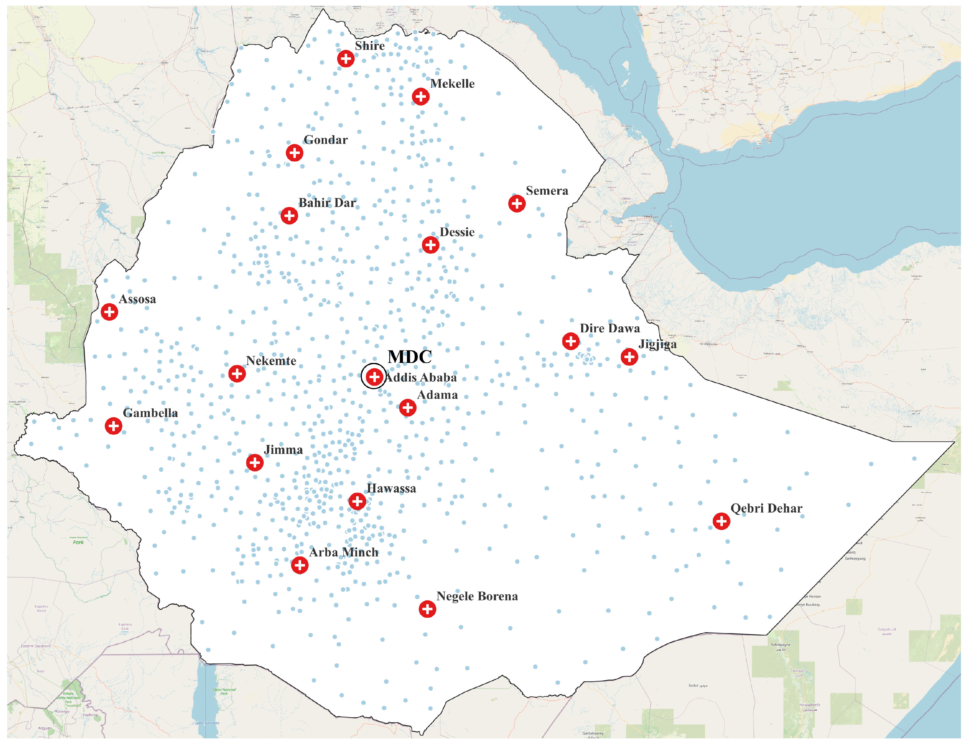
 Local distribution centers;
  Customer zones.
Local distribution centers; Customer zones.
Customer zones.
Local distribution centers; Customer zones. Selected Local DCs;
  Unselected local DCs; Customer zones.
Selected Local DCs; Unselected local DCs; Customer zones.
Unselected local DCs; Customer zones.
Selected Local DCs; Unselected local DCs; Customer zones.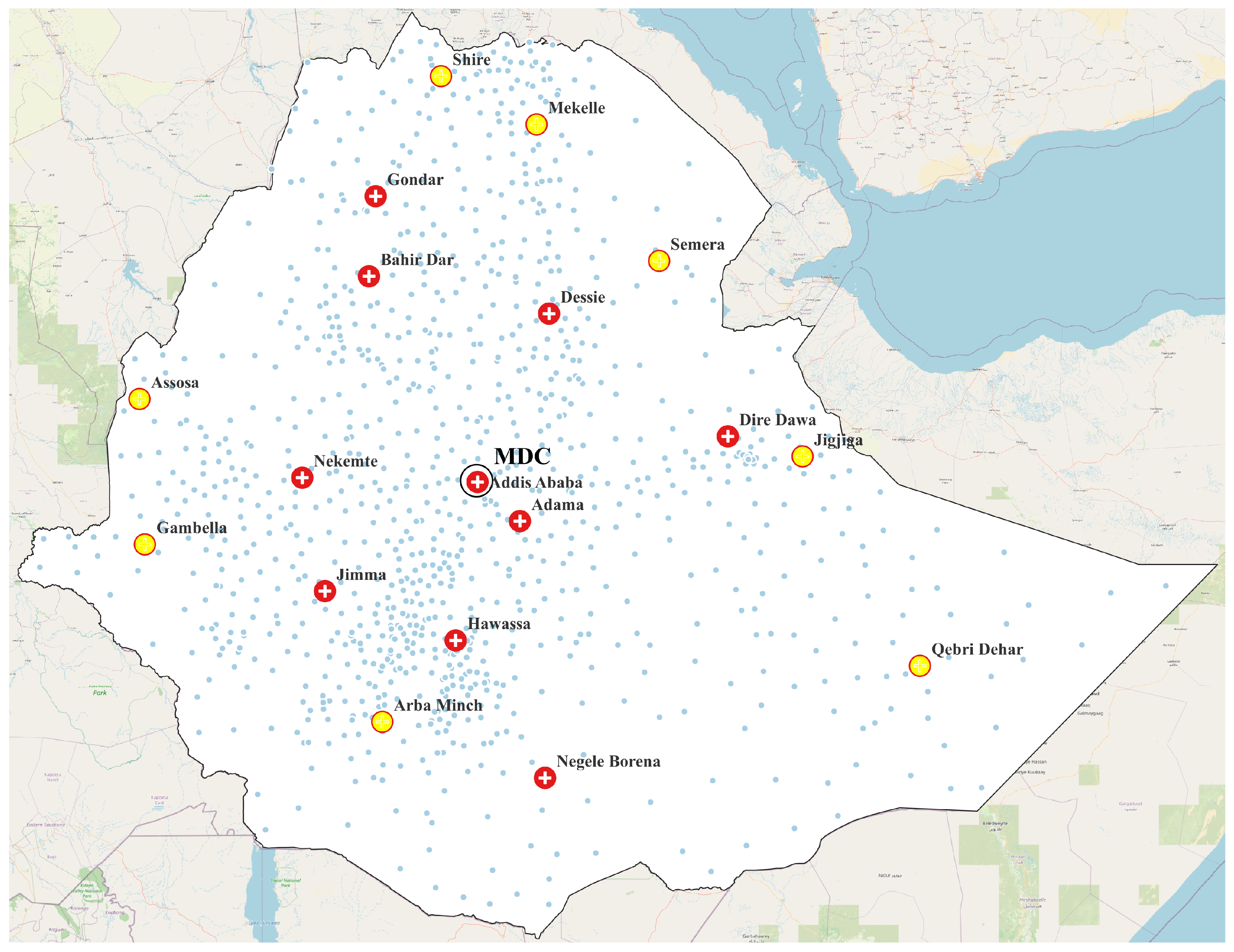

 Selected Local DCs; Unselected local DCs; Customer zones.
Selected Local DCs; Unselected local DCs; Customer zones.
Selected Local DCs; Unselected local DCs; Customer zones.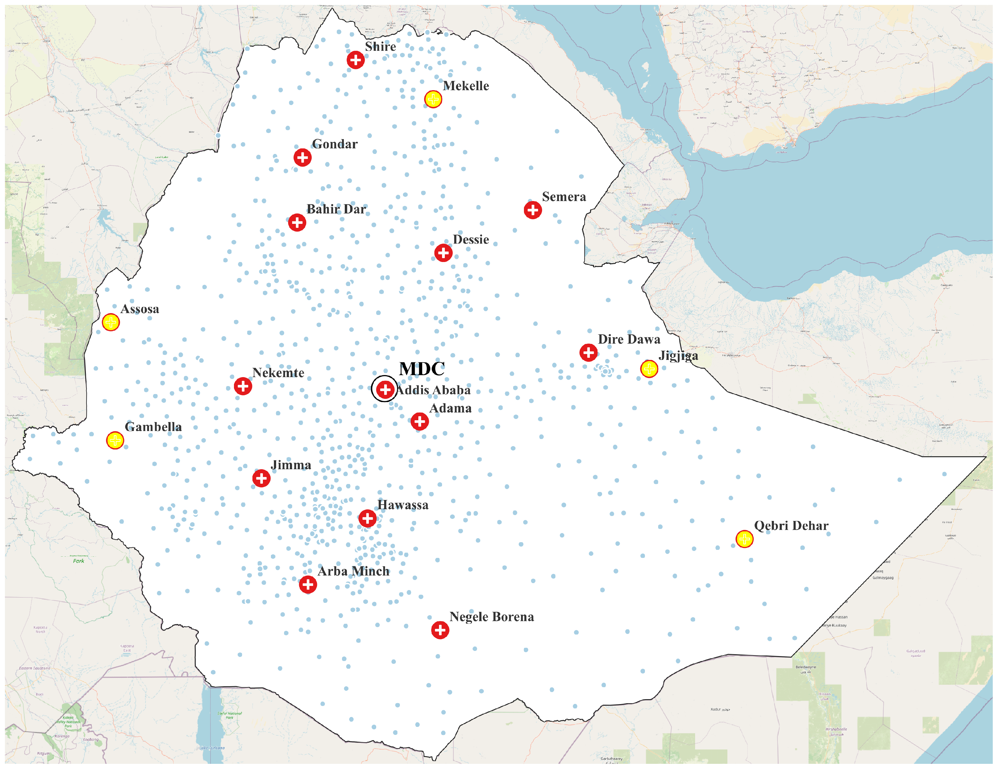
| Index Sets | |
|---|---|
| Notation | Description |
| I | Set of products indexed by i; |
| J | Set of candidate locations for local distribution center indexed by j; |
| K | Set of customer zones indexed by k; |
| S | Set of scenarios indexed by s. |
| Parameters | |
| Fixed cost of establishing local distribution center j; | |
| Per-unit cost of shipment of product i from main distribution center to local distribution center j; | |
| Per-unit cost of shipping of product i from main distribution center to customer zone k; | |
| Additional cost if a product i is delivered directly from main distribution center to customer zone k; | |
| Unit handling cost of product i at local distribution center j; | |
| Per-unit cost of shipping product i from local distribution center j to customer zone k; | |
| Demand for product i from customer zone k in scenario s; | |
| The maximum storage capacity available at local distribution center j; | |
| The minimum storage capacity allowed at local distribution center j; | |
| The maximum flow amount between main distribution and local distribution center j; | |
| The maximum flow amount between local distribution center j and customer zone k; | |
| The maximum flow amount between the main distribution center and customer zone k; | |
| Probability of occurrence of scenario s. | |
| Decision Variables | |
| Quantity of product i transported from main distribution center to local distribution center j in scenario s; | |
| Storage capacity of the local distribution center j; | |
| Quantity of product i transported from local distribution center j to customer zone k in scenario s; | |
| Quantity of product i shipped from main distribution center to customer zone k in scenario s. | |
| Binary Variables | |
| Is a binary variable, which is 1 if a facility j is to be located, and 0 otherwise; | |
| Is a binary variable, showing the link between the main distribution center and local distribution center j and 1 if the link is created, and 0 otherwise; | |
| Is a binary variable, showing the link between local distribution center j and customer zone k; it is 1 if link is to be created, and 0 otherwise; | |
| Is a binary variable, showing a link between the main distribution center and customer zone; it is 1 if the link is to be created, and 0 otherwise. | |
| S.No. | Center Name | S.No. | Center Name | S.No. | Center Name | S.No. | Center Name | S.No. | Center Name |
|---|---|---|---|---|---|---|---|---|---|
| 1 | Mekelle | 5 | Gondar | 9 | Assosa | 13 | Negele Borena | 17 | Addis Ababa 1 * |
| 2 | Shire | 6 | Jimma | 10 | Gambella | 14 | Dire Dawa | 18 | Addis Ababa 2 * |
| 3 | Semera | 7 | Nekemte | 11 | Hawassa | 15 | Jigjiga | 19 | Adama |
| 4 | Bahir Dar | 8 | Dessie | 12 | Arba Minch | 16 | Qebri Dehar |
| Code | Local Distribution Centers (LDCs) | Number of Customer Zones Assigned |
|---|---|---|
| LDC1 | Mekelle | 58 |
| LDC2 | Shire | 21 |
| LDC3 | Semera | 35 |
| LDC4 | Bahir Dar | 84 |
| LDC5 | Gondar | 36 |
| LDC6 | Jimma | 81 |
| LDC7 | Nekemte | 83 |
| LDC8 | Dessie | 67 |
| LDC9 | Assosa | 28 |
| LDC10 | Gambella | 13 |
| LDC11 | Hawassa | 150 |
| LDC12 | Arba Minch | 45 |
| LDC13 | Negele Borena | 76 |
| LDC14 | Dire Dawa | 114 |
| LDC15 | Jigjiga | 66 |
| LDC16 | Qebri Dehar | - |
| LDC17 | Addis Ababa | 154 |
| LDC18 | Adama | 72 |
| Total number of customer zones | 1029 | |
| Cost Components | Cost |
|---|---|
| Supply cost from MDC to LDCs | 1.03 × 10 |
| Delivery cost from LDCs to CZs | 5.24 × 10 |
| Handling cost at LDCs | 3.10 × 10 |
| Fixed establishment cost of LDCs | 2.37 × 10 |
| Total cost | 4.23 × 10 |
| Local Distribution Center (j) | Maximum Capacity, (Kg) | Fixed Establishment Cost, (Millions) | Local Distribution Center (j) | Maximum Capacity, (Kg) | Fixed Establishment Cost, (Millions) |
|---|---|---|---|---|---|
| 3000 | 14.5 | 3000 | 13.5 | ||
| 3000 | 9.5 | 3000 | 14 | ||
| 3000 | 13 | 3000 | 13.5 | ||
| 3000 | 15 | 3000 | 9 | ||
| 3000 | 11.5 | 3000 | 12 | ||
| 3000 | 12.25 | 3000 | 12 | ||
| 3000 | 12.5 | 3000 | 9.5 | ||
| 3000 | 14 | 3000 | 22 | ||
| 3000 | 12.5 | 3000 | 16.5 |
| Product (i) | Per Kg Handling Cost at LDC, | Product (i) | Per Kg Handling Cost at LDC, | Product (i) | Per Kg Handling Cost at LDC, | Product (i) | Per Kg Handling Cost at LDC, |
|---|---|---|---|---|---|---|---|
| 0.06250 | 0.04300 | 0.08480 | 0.03815 | ||||
| 0.94710 | 0.87475 | 0.09080 | 0.29820 | ||||
| 0.21475 | 1.82050 | 0.31305 | 0.44120 | ||||
| 1.76530 | 0.06325 | 0.23130 | 0.31310 | ||||
| 1.77405 | 0.05445 | 0.22000 | 0.68500 | ||||
| 1.78000 | 0.40030 | 0.03990 | 0.97500 | ||||
| 0.11310 | 0.16750 | 0.21355 | 0.68880 | ||||
| 0.56095 | 0.14285 | 0.65600 | 0.97660 | ||||
| 0.10720 | 0.42550 | 0.09550 | 0.06600 | ||||
| 0.22465 | 0.42425 | 0.10350 | 0.50000 | ||||
| 0.21415 | 0.34195 | 0.04685 | 0.37110 | ||||
| 0.35315 | 0.15025 | 0.61250 |
| LDC (j) | MDC | LDC (j) | MDC | LDC (j) | MDC | LDC (j) | MDC | LDC (j) | MDC | LDC (j) | MDC |
|---|---|---|---|---|---|---|---|---|---|---|---|
| 7.87 | 4.79 | 3.11 | 6.92 | 5.98 | 10.01 | ||||||
| 9.36 | 6.50 | 4.01 | 2.86 | 4.61 | 0.04 | ||||||
| 5.79 | 3.51 | 6.62 | 4.51 | 6.23 | 0.98 |
| Weight * | Obj. 1 | Obj. 2 | Integ. Gap | CPU Time |
|---|---|---|---|---|
| Highest/Lowest | 3.192619772315 × 10 | 0.00 | 0.0088% | 247.37 s |
| Equal weight | 3.192619772315 × 10 | 0.00 | 0.0088% | 242.16 s |
| Lowest/Highest | 3.192619772315 × 10 | 0.00 | 0.0088% | 242.16 s |
| First Case | Second Case | |||
|---|---|---|---|---|
| Parameters | Obj. 1 | Obj. 2 | Obj. 1 | Obj. 2 |
| Priority | Highest | Lowest | Lowest | Highest |
| Best value | 3.1924761 × 10 | 0.00 | 3.1926172 × 10 | 0.00 |
| Integrality Gap | 0.0041% | 0.0000% | 0.0090% | 0.0000% |
| CPU time (s) | 130.34 | 130.58 | 164.44 | 101.63 |
| Nodes explored | 159 | 0 | 113 | 1 |
| Variables | 818,853 continuous and 17,440 binary | |||
| Local Distribution Center (j) | Number of Customer Zones Allocated |
|---|---|
| LDC04 ≡ Bahir Dar | 66 |
| LDC05 ≡ Gondar | 72 |
| LDC06 ≡ Jimma | 114 |
| LDC07 ≡ Nekemte | 124 |
| LDC08 ≡ Dessie | 103 |
| LDC11 ≡ Hawassa | 81 |
| LDC13 ≡ Negele Borena | 82 |
| LDC14 ≡ Dire Dawa | 143 |
| LDC17 ≡ Addis Ababa | 40 |
| LDC18 ≡ Adama | 58 |
| MDC * ≡ Addis Ababa | 33 |
| Total | 916 |
| Cost Components | Model Value | Existing Value |
|---|---|---|
| Supply cost from MDC to LDCs | 1.02 × 10 | 1.03 × 10 |
| Delivery cost from LDCs to CZs | 4.67 × 10 | 5.24 × 10 |
| Direct delivery cost from MDC to CZs | 3.52 × 10 | - |
| Handling cost at LDCs | 3.10 × 10 | 3.10 × 10 |
| Fixed establishment cost of LDCs | 1.39 × 10 | 2.37 × 10 |
| Total cost | 3.19 × 10 | 4.23 × 10 |
| Scenario (s) | Definition | Probability () |
|---|---|---|
| Scenario 1 | Demand is considered to be increased by 10% | 0.20 |
| Scenario 2 | Demand is considered to be increased by 20% | 0.35 |
| Scenario 3 | Demand is considered to be increased by 30% | 0.45 |
| Weight * | Obj. 1 | Obj. 2 | Gap | CPU Time |
|---|---|---|---|---|
| Highest/Lowest | 4.941103393284 × 10 | 0.00 | 0.0075% | 2018.41 s |
| Equal weight | 4.941103393284 × 10 | 0.00 | 0.0075% | 1561.31 s |
| Lowest/Highest | 4.941103393284 × 10 | 0.00 | 0.0075% | 2027.04 s |
| First Case | Second Case | |||
|---|---|---|---|---|
| Parameters | Obj. 1 | Obj. 2 | Obj. 1 | Obj. 2 |
| Priority | Highest | Lowest | Lowest | Highest |
| Best value | 4.941115 × 10 | 0.00 | 4.941115 × 10 | 0.00 |
| Integrality Gap | 0.0079% | 0.0000% | 0.0.0079% | 0.0000% |
| CPU time (sec) | 541.27 | 543.03 | 684.70 | 279.95 |
| Nodes explored | 1145 | 0 | 1145 | 1 |
| Variables | 2,456,521 continuous and 17,440 binary | |||
| Local Distribution Center (j) | Number of Customer Zones Allocated |
|---|---|
| LDC03 ≡ Semera | 95 |
| LDC04 ≡ Bahir Dar | 47 |
| LDC05 ≡ Gondar | 58 |
| LDC06 ≡ Jimma | 95 |
| LDC07 ≡ Nekemte | 79 |
| LDC08 ≡ Dessie | 66 |
| LDC09 ≡ Assosa | 58 |
| LDC11 ≡ Hawassa | 60 |
| LDC12 ≡ Arba Minch | 78 |
| LDC13 ≡ Negele Borena | 88 |
| LDC14 ≡ Dire Dawa | 109 |
| LDC17 ≡ Addis Ababa | 17 |
| LDC18 ≡ Adama | 40 |
| MDC * ≡ Addis Ababa | 26 |
| Total | 916 |
| Weight * | Obj. 1 | Obj. 2 | Gap | CPU Time |
|---|---|---|---|---|
| Highest/Lowest | 4.821993464381 × 10 | 0.00 | 0.0098% | 8944.20 s |
| Equal weight | 4.821993464381 × 10 | 0.00 | 0.0098% | 6580.38 s |
| Lowest/Highest | 4.821993464381 × 10 | 0.00 | 0.0098% | 7325.70 s |
| First Case | Second Case | |||
|---|---|---|---|---|
| Parameters | Obj. 1 | Obj. 2 | Obj. 1 | Obj. 2 |
| Priority | Highest | Lowest | Lowest | Highest |
| Best value | 4.8219831 × 10 | 0.00 | 4.8219786 × 10 | 0.00 |
| Integrality Gap | 0.0092% | 0.0000% | 0.0090% | 0.0000% |
| CPU time (s) | 10,890.21 | 10,891.44 | 10,031.69 | 594.60 |
| Nodes explored | 30,180 | 0 | 35,519 | 1 |
| Variables | 2,456,521 continuous and 52,284 binary | |||
| Number of CZs Allocated in Each Scenario | |||
|---|---|---|---|
| Local Distribution Center (j) | s = 1 | s = 2 | s = 3 |
| LDC02 ≡ Shire | 2 | 23 | 44 |
| LDC03 ≡ Semera | 39 | 61 | 96 |
| LDC04 ≡ Bahir Dar | 58 | 55 | 53 |
| LDC05 ≡ Gondar | 70 | 58 | 54 |
| LDC06 ≡ Jimma | 114 | 105 | 96 |
| LDC07 ≡ Nekemte | 106 | 103 | 88 |
| LDC08 ≡ Dessie | 76 | 69 | 59 |
| LDC11 ≡ Hawassa | 75 | 68 | 54 |
| LDC12 ≡ Arba Minch | 84 | 87 | 83 |
| LDC13 ≡ Negele Borena | 49 | 83 | 85 |
| LDC14 ≡ Dire Dawa | 136 | 113 | 109 |
| LDC17 ≡ Addis Ababa | 41 | 32 | 28 |
| LDC18 ≡ Adama | 39 | 30 | 26 |
| MDC * ≡ Addis Ababa | 27 | 29 | 41 |
| Total | 916 | 916 | 916 |
| Cost Values in Each Scenario (in Relative Money Units) | |||
|---|---|---|---|
| Cost Components | s = 1 | s = 2 | s = 3 |
| Supply cost (MDC to LDCs) | 1.16 × 10 | 1.35 × 10 | 1.55 × 10 |
| Delivery cost (LDCs to CZs) | 4.90 × 10 | 5.35 × 10 | 6.24 × 10 |
| Material handling cost (at LDCs) | 3.41 × 10 | 3.72 × 10 | 4.03 × 10 |
| Fixed establishment cost (of LDCs) | 1.75 × 10 | ||
| Direct delivery cost (MDC to CZs) | 5.45 × 10 | 5.00 × 10 | 3.16 × 10 |
| Additional cost at MDC | 2.13 × 10 | 1.97 × 10 | 3.62 × 10 |
Disclaimer/Publisher’s Note: The statements, opinions and data contained in all publications are solely those of the individual author(s) and contributor(s) and not of MDPI and/or the editor(s). MDPI and/or the editor(s) disclaim responsibility for any injury to people or property resulting from any ideas, methods, instructions or products referred to in the content. |
© 2023 by the authors. Licensee MDPI, Basel, Switzerland. This article is an open access article distributed under the terms and conditions of the Creative Commons Attribution (CC BY) license (https://creativecommons.org/licenses/by/4.0/).
Share and Cite
Gobachew, A.M.; Haasis, H.-D. Scenario-Based Optimization of Supply Chain Performance under Demand Uncertainty. Sustainability 2023, 15, 10603. https://doi.org/10.3390/su151310603
Gobachew AM, Haasis H-D. Scenario-Based Optimization of Supply Chain Performance under Demand Uncertainty. Sustainability. 2023; 15(13):10603. https://doi.org/10.3390/su151310603
Chicago/Turabian StyleGobachew, Asrat Mekonnen, and Hans-Dietrich Haasis. 2023. "Scenario-Based Optimization of Supply Chain Performance under Demand Uncertainty" Sustainability 15, no. 13: 10603. https://doi.org/10.3390/su151310603