Abstract
Distracted driving leads to a significant number of road crashes worldwide. Smartphone use is one of the most common causes of cognitive distraction among drivers. Available data on drivers’ phone use presents an invaluable opportunity to identify the main factors behind this behavior. Machine learning (ML) techniques are among the most effective techniques for this purpose. However, the potential and usefulness of these techniques are limited, due to the imbalance of available data. The majority class of instances collected is for drivers who do not use their phones, while the minority class is for those who do use their phones. This paper evaluates two main approaches for handling imbalanced datasets on driver phone use. These methods include oversampling and undersampling. The effectiveness of each method was evaluated using six ML techniques: Multilayer Perceptron (MLP), Support Vector Machine (SVM), Naive Bayes (NB), Bayesian Network (BayesNet), J48, and ID3. The proposed methods were also evaluated on three Deep Learning (DL) models: Arch1 (5 hidden layers), Arch2 (10 hidden layers), and Arch3 (15 hidden layers). The data used in this document were collected through a direct observation study to explore a set of human, vehicle, and road surface characteristics. The results showed that all ML methods, as well as DL methods, achieved balanced accuracy values for both classes. ID3, J48, and MLP methods outperformed the rest of the ML methods in all scenarios, with ID3 achieving slightly better accuracy. The DL methods also provided good performances, especially for the undersampling data. The results also showed that the classification methods performed best on the undersampled data. It was concluded that road classification has the highest impact on cell phone use, followed by driver age group, driver gender, vehicle type, and, finally, driver seatbelt usage.
1. Introduction
Road crashes are considered one of the biggest challenges faced by countries and societies in our modern era, due to the vast human losses and material damage that may result from these crashes. The World Health Organization (WHO) reported that road traffic injuries are among the leading causes of mortality for children and young adults aged between 5 and 29 years [1]. Approximately 1.3 million individuals are killed in road traffic accidents. According to WHO records, road traffic accidents cost countries 3% of their gross domestic product (GDP).
With the rise of cell devices and smartphones, and people’s growing reliance on them in most parts of their lives, there have been more car crashes caused by this new technology. Using phones while driving leads to distracted driving, which is one of the main factors leading to serious road crashes. According to WHO, mobile phone users are roughly four-fold more probable to be part of road crashes [2]. Using a phone while driving contributes to slowing down drivers’ reactions, increasing lane deviations, and making drivers look away from the steering wheel for extended periods. Despite the existence of strict laws in most countries, including Jordan, to deter drivers from using their phones, the number of crashes involving the use of phones is steadily increasing. Hence, studying the possible reasons that make some drivers more likely to use phones than others is one of the best approaches to finding a solution to this dilemma.
Machine learning (ML) techniques have recently gained attention in analyzing traffic-related datasets [3,4,5,6,7,8,9,10,11,12]. The ability of these techniques to deal with large datasets, and to identify the relationships among variables that would be extremely difficult to identify directly with the standard statistical modeling approaches, makes them appealing for researchers to employ. Classification algorithms are among the most widely used ML techniques for analyzing traffic-related datasets. Classification is a supervised learning technique that uses training data to predict the class of new occurrences. In classification, a program is trained on a given dataset to classify new observations into several classes or groups. The generated classifiers can be used as predictors for future observations and, in some classification algorithms (e.g., decision trees), can extract some rules that traffic agencies can employ to understand the drivers’ mentalities better.
Almost all datasets about traffic have the problem of imbalanced data. In the case of the phone usage dataset, the data for drivers using their phones are underrepresented compared with those who do not use their phones. Unfortunately, ML tools are designed to achieve their best performance on balanced datasets, an assumption that is not always true. Another assumption such tools make is that the desired goal should be maximizing classification accuracy. Under these assumptions, classifiers tend to disregard the minority class and predict all instances into the majority class, achieving a high level of classification accuracy. Such classifiers are obviously not practical.
Therefore, any attempt to apply classification techniques to traffic-related data must first address the issue of imbalance, inherent in this type of data. This paper evaluates two significant techniques for handling an imbalanced dataset for drivers’ phone use in Jordan. These techniques are undersampling and oversampling. Data used in this paper were collected via a direct observational survey, covering a set of characteristics associated with three main safety aspects: humans, vehicles, and roadways [13]. The effectiveness of each technique was evaluated by applying six ML methods and three DL architectures on the balanced data. The ML techniques are Multilayer Perceptron (MLP), Support Vector Machine (SVM), Decision Tree (ID3), Decision Tree (J48), Bayesian Network (BayesNet), and Naive Bayes (NB). The DL architecture are: Archt1 (5 hidden dense layers), Archt2 (10 hidden dense layers), and Archt3 (15 hidden dense layers).
2. Related Work
Data collected about drivers represents a valuable source of knowledge for traffic agencies and traffic researchers. Analyzing such data can help recognize patterns in reckless, unsafe behaviors, such as using cell phones and not wearing seatbelts. Raman et al. (2014) [14] investigated the factors associated with using seatbelts and cellphones and the levels of possible unsafe driving behaviors in 741 adult drivers and front-seat occupants in Kuwait. Results showed that dangerous driving behaviors were prevalent, including seatbelt use (41.6%), cellphone use (‘always’ or ‘almost always’: 51.1%), and texting (32.4%).
Some effective analyzing tools need to be employed to extract knowledge from these data, which is characterized by their large volume and multidimensionality. Researchers have recently gained interest in ML methods for analyzing driver-related datasets. The ability of these methods to deal with large datasets and determine interactions between large numbers of variables makes them a good fit for road traffic-related datasets. However, for such methods to be effective, the data needs to be balanced. Unfortunately, most traffic-related datasets are imbalanced, which significantly affects the performance of the ML tools. Numerous studies have been conducted to resolve the problem of imbalanced road-related datasets before applying ML methods. Two significant techniques were mainly used in these studies: oversampling and undersampling.
Fiorentini and Losa (2020) [15] used a method called “random undersampling” to deal with crash datasets that were not balanced. Four ML methods were then applied to the balanced data. These methods are Random Tree, k-Nearest Neighbor, Logistic Regression, and Random Forest. The findings demonstrated that using the undersampling technique enhanced the accuracy of the classifiers for predicting fatal and injury-causing accidents. Another study proposed an ensemble learning-based undersampling technique using Extreme Gradient Boosting (XGBoost) and Support Vector Machine (SVM) [16]. The proposed technique was implemented on a crash dataset, and the outcomes indicated that it was able to resolve the problem of class imbalance. The same technique was used by Shi et al. (2019) [17] to reduce the risk-safe class imbalance in a dataset about driving behaviors. The aim was to build a classifier for predicting risk levels. The XGBoost technique was used for building that classifier, which performed very effectively. The Synthetic Minority Oversampling Technique (SMOTE) was used to overcome the issue of an imbalanced dataset of car crashes [18,19]. SVM and NN were then applied to the balanced data set, and the results showed that NN outperformed SVM. A new model, called Deep Convolutional Generative Adversarial Network (DCGAN), was proposed by Cai et al. (2020) [20] to generate more synthetic data related to crashes to balance the dataset. The performance of the proposed model was compared with that of random undersampling and SMOTE. Several crash prediction models were then applied to the balanced dataset. The findings revealed that the convolutional neural network model developed using the DCGAN balanced data could deliver the highest prediction accuracy.
Several studies compared different sampling techniques to choose the best one for the classification models [21,22,23,24,25,26,27]. Random undersampling, SMOTE, and a mix of both were used by Boonserm and Wiwatwattana (2021) [22] prior to applying the random forest technique to a dataset of traffic crashes. The result showed that random undersampling provided the best performance. Similarly, Mujalli et al. (2016) [23] used the same sampling techniques to evaluate the performance of various Bayes classifiers. However, the results revealed that the classifiers worked better on the oversampled data. A mix of undersampling and SMOTE techniques were used by Schlögl et al. (2019) [28] to balance a dataset of traffic crashes. Subsequently, a series of classification methods were applied to the balanced data. Results showed satisfying performance of tree-based methods, with 75% and 90% accuracy. Random oversampling, SMOTE, and adaptive synthetic sampling were explored by Morris and Yang (2021) [24]. The performance of these sampling techniques was evaluated using three ensemble ML models (CatBoost, XGBoost, and Random Forest). According to the findings, all three sampling approaches improved the performance of all models. However, the adaptive synthetic sampling method outperformed the other two oversampling methods. Random undersampling and SMOTE oversampling techniques were applied to a crash dataset by Bedane et al. (2021) [25] to address the class imbalance of the dependent attributes. This was followed by applying seven classification methods. The results showed that Random Forest performed best with the SMOTE oversampled dataset. Both undersampling and oversampling were also used by Jeong et al. (2018) [26] for the same purpose. Several classification methods were then applied to the data, and the results indicated that the decision trees performed the best with oversampling treatment for imbalanced data. The performance of convolutional neural networks was assessed using different sampling techniques by Basso et al. (2021) [27]. The undersampling technique was found to provide the best results.
The conclusion that can be drawn from the literature is that no particular sampling technique can be recommended for all kinds of datasets. Some studies found that random undersampling worked best for them, while others showed that SMOTE was the best for balancing the datasets. Indeed, some researchers proposed novel sampling techniques that worked best for their dataset. Therefore, the best way to find the most suitable sampling technique is by trying them all, which is precisely what we plan to do in this paper.
3. Materials and Methods
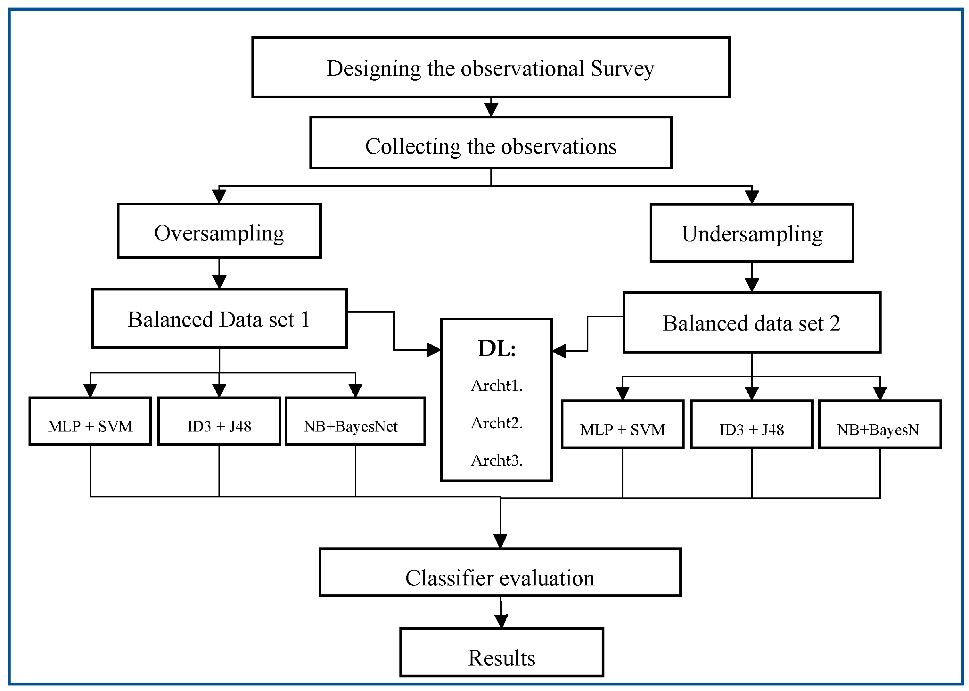
In this section, we will first provide an overview of how the data used in this paper were obtained. Then, the oversampling and undersampling techniques are used on the initial dataset to handle the imbalanced classes. The balanced dataset is then used as an input for six ML techniques and three DL architectures to build classification models. The ML techniques include MLP, SVM, ID3, J48, NB, and BayesNet. The DL architectures are Archt1 (5 hidden layers), Archt2 (10 hidden layers), and Archt3 (15 hidden layers). Finally, the models are evaluated, and the results are reported. The overall workflow of the methodology is presented in Figure 1.
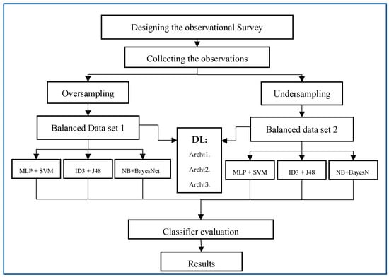
Figure 1.
Methodology Workflow.
3.1. Data Collection
The dataset used in this study was gathered from three major Jordanian cities, namely Amman, Irbid, and Zarqa. The reason behind selecting these cities is their high population and the large number of registered vehicles in comparison to other Jordanian cities. A direct observational survey was used to collect the data. Data collection covered every hour between 7 a.m. and 7 p.m., every day of the week, in Spring 2017. Upon revisiting the field with careful observation, the years 2017–2023 have remained the same. The drivers continue to exhibit the same behaviors as before. Additionally, there have been no traffic campaigns targeting driver behavior while driving since 2017 in Jordan. Three thousand and two hundred vehicles were observed. Observations were accomplished by standing at the side of the roadway or while driving a vehicle. It is crucial to prioritize safety to minimize any risks or accidents. Therefore, several safety measures were considered, including staying alert, avoiding distractions, choosing a safe location, using proper equipment (e.g., a clipboard, paper, pen, or a mobile device), following traffic rules, considering weather conditions, and communicating with local authorities. The descriptions of all the information collected about each observation are shown in Table 1. As noted, each observation includes a group of characteristics covering the three major safety elements: human, vehicle, and roadway.

Table 1.
Description of All Attributes in the Dataset.
3.2. Imbalanced Dataset Handling Techniques
As can be noted from Figure 2, the drivers using their cell phones are underrepresented in the data set. The percentage of these drivers is only 15% of all the drivers. Applying the classification techniques to such a dataset will result in biased classifiers. The generated classifiers tend to simply disregard the minority class and predict everything into the majority class, as this guarantees high classification accuracy. The accuracy of the classification algorithms used in this paper on the initial dataset is presented in Table 2. The equations for calculating the accuracy are explained in the Results section.
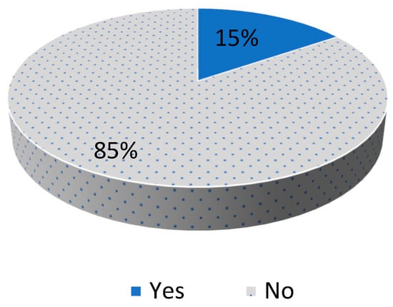
Figure 2.
Distribution of Cell Phone Usage in the Dataset.
Table 2.
Accuracy of the Classification Algorithms on the Initial Dataset.
It is evident from Table 2 that, despite the high accuracy achieved by all classification algorithms, the performance is poor for the minority class (i.e., Yes). These kinds of classifiers are misleading and not helpful. It is, therefore, necessary to handle the imbalanced dataset before applying the classification techniques. Two techniques were used in this paper to address imbalanced data: oversampling and undersampling.
3.2.1. Oversampling
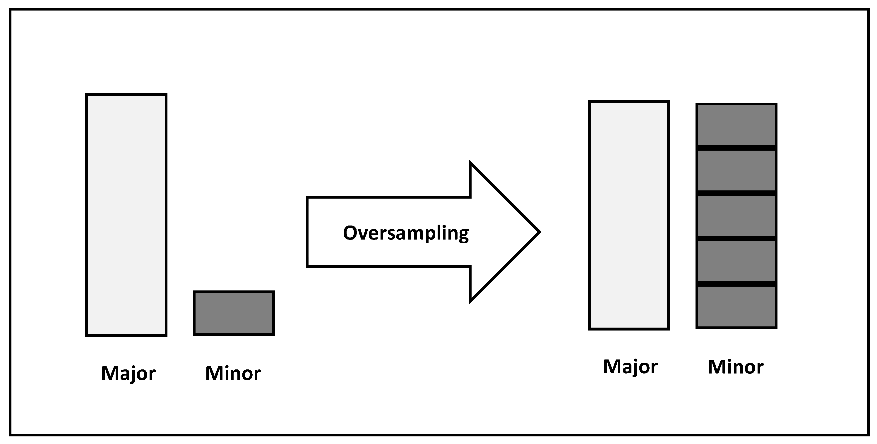
Figure 3 depicts Oversampling as a technique used in ML for handling imbalanced datasets. Imbalanced datasets are characterized by having one class of the target variable (minority class) represented by significantly fewer observations than the other class (majority class). Models trained on such datasets tend to be skewed towards the majority class and perform inadequately in the minority class.
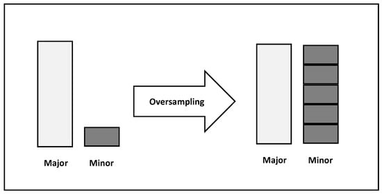
Figure 3.
Oversampling.
Oversampling aims at increasing the number of instances in the minority class to balance the dataset. This can be done either by randomly duplicating existing observations in the minority class or by synthetically generating new observations. The former is called resampling, while the latter is called Synthetic Minority Oversampling Techniques (SMOTE).
SMOTE creates synthetic samples in the minority class based on the feature space of existing minority class samples. Specifically, it selects a sample from the minority class and finds its k-nearest neighbors (i.e., the k samples in the minority class that are closest to it). It then randomly selects one of these neighbors and creates a new sample that is a linear combination of the original samples and the selected neighbor. The process is repeated until the desired number of synthetic samples is generated. In this paper, both resampling and SMOTE are used.
3.2.2. Undersampling
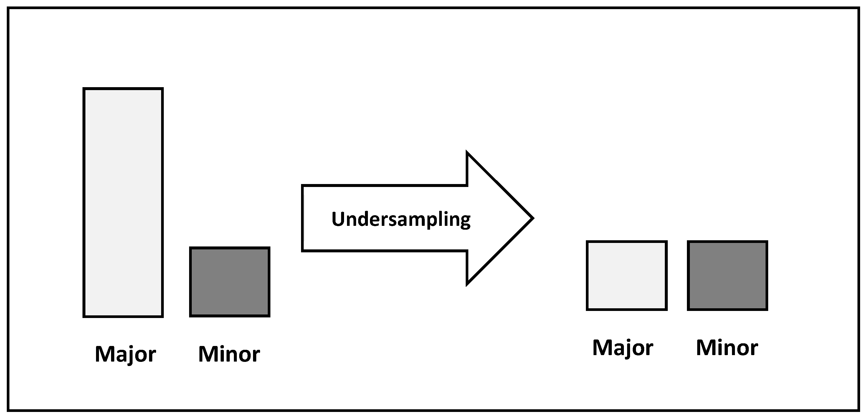
Another technique used for handling imbalanced datasets is undersampling. Undersampling involves reducing the number of instances in the majority class to balance the dataset (see Figure 4). This can be done by randomly selecting a subset of instances from the majority class to roughly equal the number of instances in each class.

Figure 4.
Undersampling.
Undersampling can be a simple and effective approach for dealing with class imbalance, especially when the dataset is very large and oversampling techniques may be computationally expensive. However, undersampling may also result in losing important information from the majority class(es) and may not work well if the minority class(es) is too small.
3.3. Classification Methods
Six ML techniques and three DL architectures were applied to the balanced dataset to evaluate the performance of each class imbalance handling method. The ML techniques are two Bayes classifiers (Naive Bayes and Bayesian Network), two function-based classifiers (Multilayer Perceptron and Support Vector Machine), and two decision tree-based classifiers (ID3 and J48). The DL architectures are presented in Table 3.
Table 3.
The Deep Learning Architectures Evaluated on the Sampled Data.
3.3.1. Naive Bayes (NB)
Naïve Bayes (NB) is a classification technique that utilizes the Bayesian theorem. The NB technique assumes that all variables are independent. Even though this assumption is too oversimplified, NB has proven effective in many real-world problems. Specifically, NB was used for sorting documents and spam filtering. Additionally, NB was found to be exceptionally quick at learning and predicting data. Bayes’ theorem is a straightforward method for computing conditional probabilities. It calculates the probability of an event based on the probability of another event that has already occurred, and this relationship is mathematically expressed by the following equation:
For a dataset, the formula can be rewritten as:
where y is the target variable, X represents the features X = (x1, x2, x3,…, xn). Now, given that Naive Bayes assumes that all variables are independent, the formula can be rewritten as:
The denominator remains constant for a given input. Therefore, it can be removed:
The objective now is to identify the class variable y with the highest probability:
3.3.2. Bayesian Network (BayesNet)
BayesNet is a probabilistic graphical model in which a group of variables and their conditional dependence are represented as a Directed Acyclic Graph (DAG). In such a graph, nodes represent variables, while edges represent conditional dependencies. Each node has conditional distribution P(Xi|Parent(Xi)), which shows the impact of the parent on the node. BayesNet is based on joint probability distribution. Suppose that x1, x2, x3,…, xn are variables from a data set; then, the joint probability distribution is expressed as follows:
3.3.3. Decision Tree (ID3)
The decision tree is a data mining and ML method for building classifiers based on historical datasets. The output of this technique is a prediction model capable of identifying the value of a target variable, given the values of other input variables. The prediction models are in the form of a tree, where each interior node represents an input variable with several edges identical to the possible values that variable might have. Each leaf node contains the predicted value for the target variable, given the values of the input variables from the root of the tree down to the leaf node. The input variables that appear first in the tree are called primary splitters. A splitter node is considered very crucial in identifying the value of the target variable if it is connected directly with leaf nodes. There is a different algorithm for building a decision tree. In this paper, the Iterative Dichotomiser 3 (ID3) was employed. In ID3, a top-down, greedy search is used for teaching each attribute at each node to construct the decision tree. The best attribute at each iteration is selected using the Information Gain (IG). IG reflects the reduction in entropy and specifies how well a given feature can separate the target classes. Entropy is the measure of disorder in the target feature. Entropy is calculated as follows:
where S is the dataset for which the entropy is being calculated, c is the total number of classes in the target feature, and Pi is the probability of class i (i.e., the ratio of rows with class i to the total number of rows in the dataset).
The IG for feature A is calculated as:
where n is the total possible values for feature A, the rows in SV where A has value v, |SV| the total number of rows in SV, and |S| the total number of rows in S.
3.3.4. J48 Algorithm
J48 is another top-down, greedy algorithm based on the ID3 algorithm. The information gain is also used here to choose the attribute at each stage. The J48 algorithm builds the decision tree in the same way the ID3 does. The advantage of using this algorithm is that it can handle missing values, and continues value ranges and decision tree pruning.
3.3.5. Support Vector Machine (SVM)
SVM is a supervised learning method for classification and regression. The aim of SVM is to find a hyperplane in N-dimensional space (N is the number of features) that best separate classes. Separating two classes can be achieved by several possible hyperplanes, but the goal of SVM is to find the plane with the maximum margin (i.e., the optimal hyperplane). SVM uses a technique called the kernel trick to convert non-separable data into separable data by adding more dimensions to it. In this paper, the Radial Basis Function (RBF) kernel is used for that purpose. Here is the equation for the RBF kernel:
where gamma > 0 and is the Euclidean distance between two points and .
3.3.6. Multilayer Perceptron (MLP)
The Artificial Neural Network (ANN) is an ML method used for constructing prediction models. Such models are trained on historical datasets and are designed to predict the value of the target attribute, given the values of the input attributes. An ANN has several layers of connected nodes. These layers are classified into three types of layers: (1) input layer: each node in this layer represents an input variable; (2) hidden layer: each ANN can have zero or more hidden layers; (3) output layer: each node represents an output variable (typically one). Each node receives a value, performs some operations, and passes the output to another node. An integer value controlling the signal between nodes is used to assign a weight for each link. ANNs gain knowledge through the process of selecting the best solution. This knowledge leads to modifications in the weight values.
A feedforward ANN method, called Multilayer Perceptron (MLP), is used in this paper. An MLP network consists of three or more fully connected layers. A node in MLP is a neuron that applies a nonlinear activation function to generate the output of that node, given a set of inputs. The logistic function is used in the MLP as the activation function. This function is a sigmoid function, expressed as:
The backpropagation algorithm is used by MLP for training the network. In this algorithm, the weight values are modified after handling each instance. The goal for MLP is to find a solution for the least mean squares minimization function:
where dj is the needed output, and aj is generated by the jth output neuron. The weights are altered by calculating local gradient (δ) and moving reversely:
where n is the training repeat, η is the learning rater parameter, and α is the momentum constant.
3.3.7. Deep Learning (DL)
Deep learning is a machine learning technique that teaches computers to gain knowledge in the same way humans do. Deep learning is based on neural network with three or more layers of neurons that work together to solve a problem. DeepLearning4J is a java-based, open-source, distributed deep learning toolkit for building and training deep learning models. DeepLearning4J provides users with the capability to specify the sequence of layers that build the neural network architecture. In this paper, the deep learning models were built using the DeepLearning4J toolkit. All deep learning models consist of several dense layers and one output layer. All neurons in a dense layer are connected to all neurons of their parent layer; therefore, it is a fully connected layer. The output layer generates classification output. Table 3 presents the architectures used to train the deep learning models.
4. Results and Discussion
Three balanced versions of the dataset were generated: one using the undersampling technique, and two using the oversampling techniques (i.e., resampling and SMOTE). The classification techniques were subsequently run on all the datasets, and the results were extracted. The 10-fold cross-validation scheme was used to build the classifiers. In this scheme, the data is randomly divided into ten equal-sized subsets. These subsets are used to build ten models, where each model is built using one subset for testing the model, and the rest of the subsets are used for training. Eventually, each subset is used exactly once for testing. The results generated by all models are finally averaged.
The classifier performance is computed using the confusion matrix. In this matrix, the number of observations correctly and incorrectly predicted by the model for each class are presented. A confusion matrix for a classifier with two classes (i.e., positive and negative) is shown in Table 4. The definition of TP, TN, FP, and FN is provided below:
Table 4.
Confusion Matrix.
- True Positive (TP): +VE observations predicted as +VE.
- True Negative (TN): −VE observations predicted as −VE.
- False Positive (FP): −VE observations predicted as +VE.
- False Negative (FN): +VE observations predicted as −VE.
The performance of the classifiers is evaluated using measures computed from the confusion matrix. The accuracy rate (or precision) is among the most widely used measures for model evaluation. The higher the accuracy is, the better the model performs. The accuracy is defined as the ratio of the correctly predicted observations to the total number of observations, calculated as follows:
The performance of the classifier in each class is also important. Some important evaluation measures for this reason include the True Positive Rate (TPR), the False Positive Rate (FPR), and the Receiver Operating Characteristic (ROC) curve. The model performance increases as the TPR and Precision values increase and FPR value decreases. The mathematical formula for each measure for class positive in Table 4 is demonstrated below.
The TPR (i.e., Recall) is the ratio of observations that are positive and predicted as positive to all positive observations. It is worth mentioning here that the overall model accuracy is computed by finding the weighted average of all TPR values.
The precision is the ratio of observations that are positive and predicted as positive to all observations predicted as positive:
The False Positive Rate (FPR) or (1 − specificity) is the ratio of observations that are negative but predicted as positive to all observations that are not positive:
Finally, the ROC curve plots the TPR against the FPR at different threshold levels, which reflects the tradeoff between the benefits (i.e., TPR) and the costs (i.e., FPR). The area under the ROC curve (AUC) is used to measure the accuracy of the classification model. The AUC values range from 0.0 to 1.0, where 1.0 is the optimal case.
The performance of ID3, J48, NB, BayesNet, MLP, and SVM on the undersampled and oversampled data is presented in Table 5. The total accuracy was computed for each model. The recall, precision, and FPR were also computed for each class. As can be noted from Table 5, the ID3, J48, and MLP methods outperformed the other methods in all scenarios. The ID3 and MLP methods achieved slightly better performance than the J48 method on the undersampled data, while the ID3 and J48 methods were better than the MLP on the oversampled data. The SVM outperformed the NB and BayesNet, which performed identically on all the data. The SVM achieved its best performance on the oversampled data using SMOTE, and was close to MLP.
Table 5.
Performance of ID3, J48, NB, BayesNet, SVM, and MLP on the Undersampled and Oversampled Data.
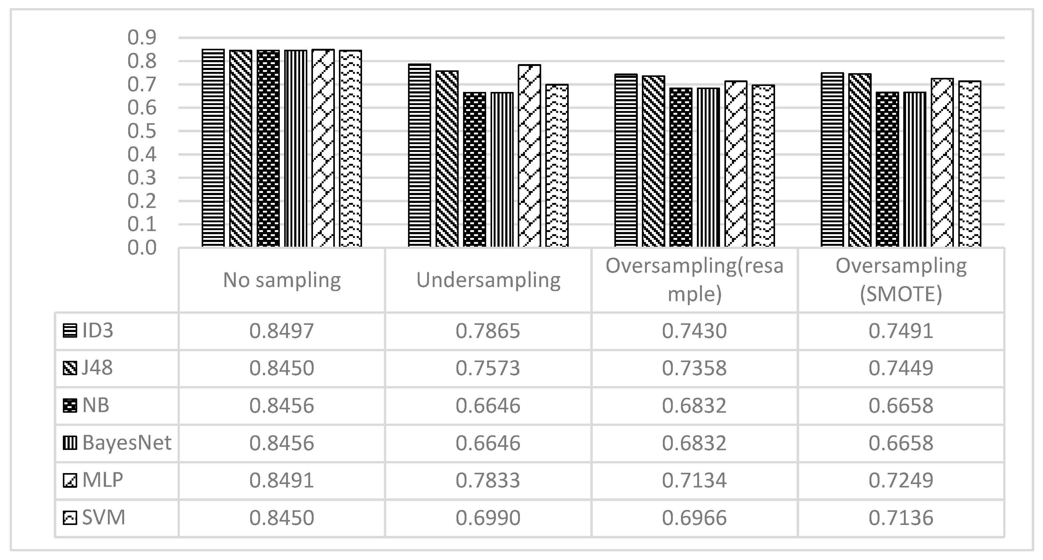
Figure 5 provides a graphical representation of the accuracy achieved by all classification models. Please note that, while the best overall accuracy was achieved when no sampling technique was used, the recall values are biased toward the majority class (i.e., not using cell phone).
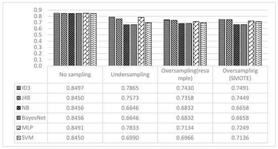
Figure 5.
Accuracy Achieved by all Classification Models.
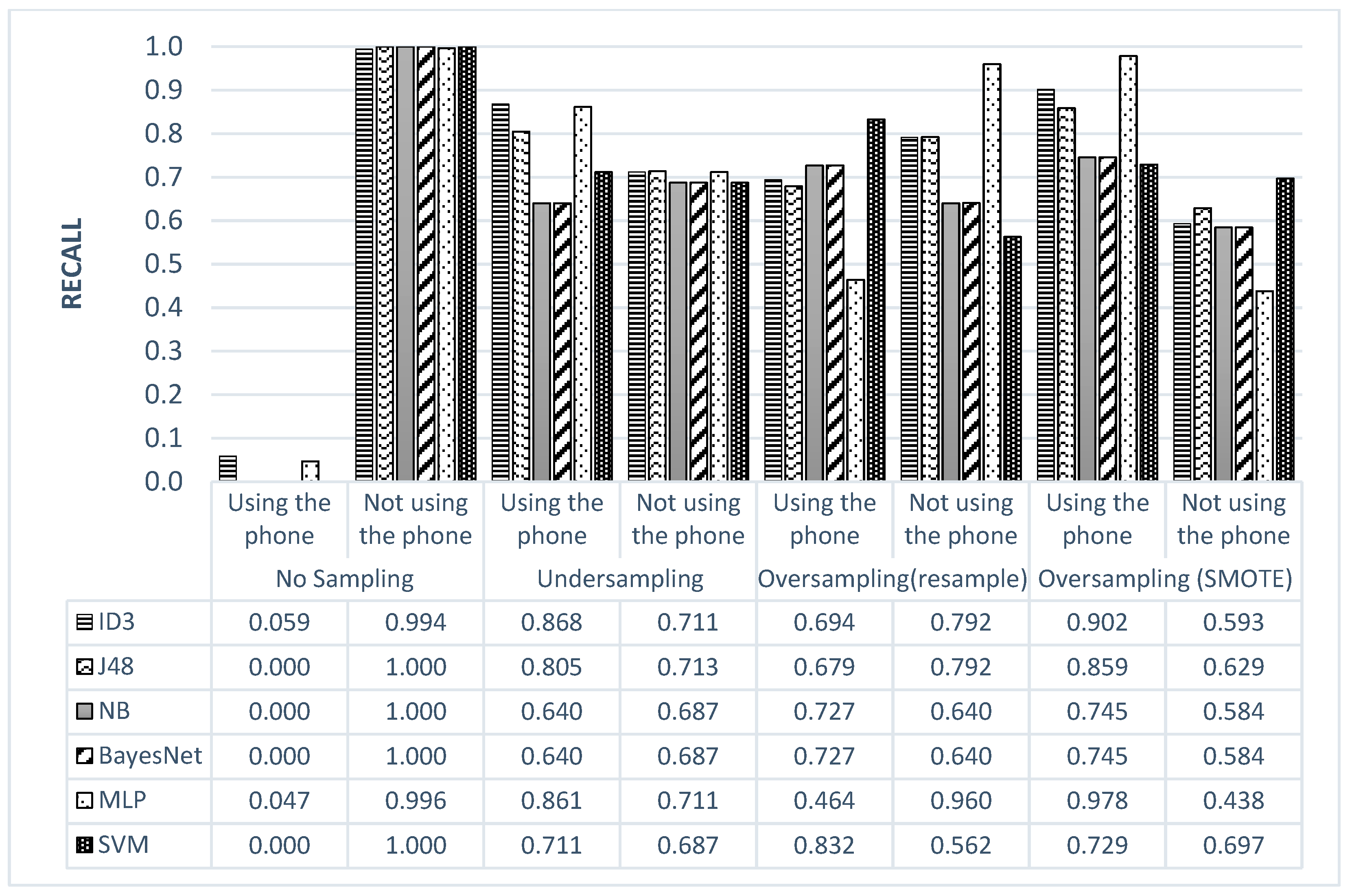
As shown in Figure 6, when no sampling technique was used, the recall values for the minority class (i.e., not using cell phone) were close to zero in all classification models. Using sampling techniques, the recall values were drastically improved. The undersampling technique provided the most balanced recall values for the majority and minority classes. Among the classification techniques applied to the undersampled data, the ID3 and MLP provided the best recall values, with a slight preference for the former method. Although MLP achieved a high recall rate for the no phone-use class on the oversampled data using the resampling technique, the other class (phone-use class) witnessed a considerable drop in the same value. The same observation can be made on the oversampled data using SMOTE, but with the phone-use class having a high recall rate.
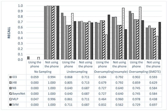
Figure 6.
Recall Values for Each Class for All Scenarios.
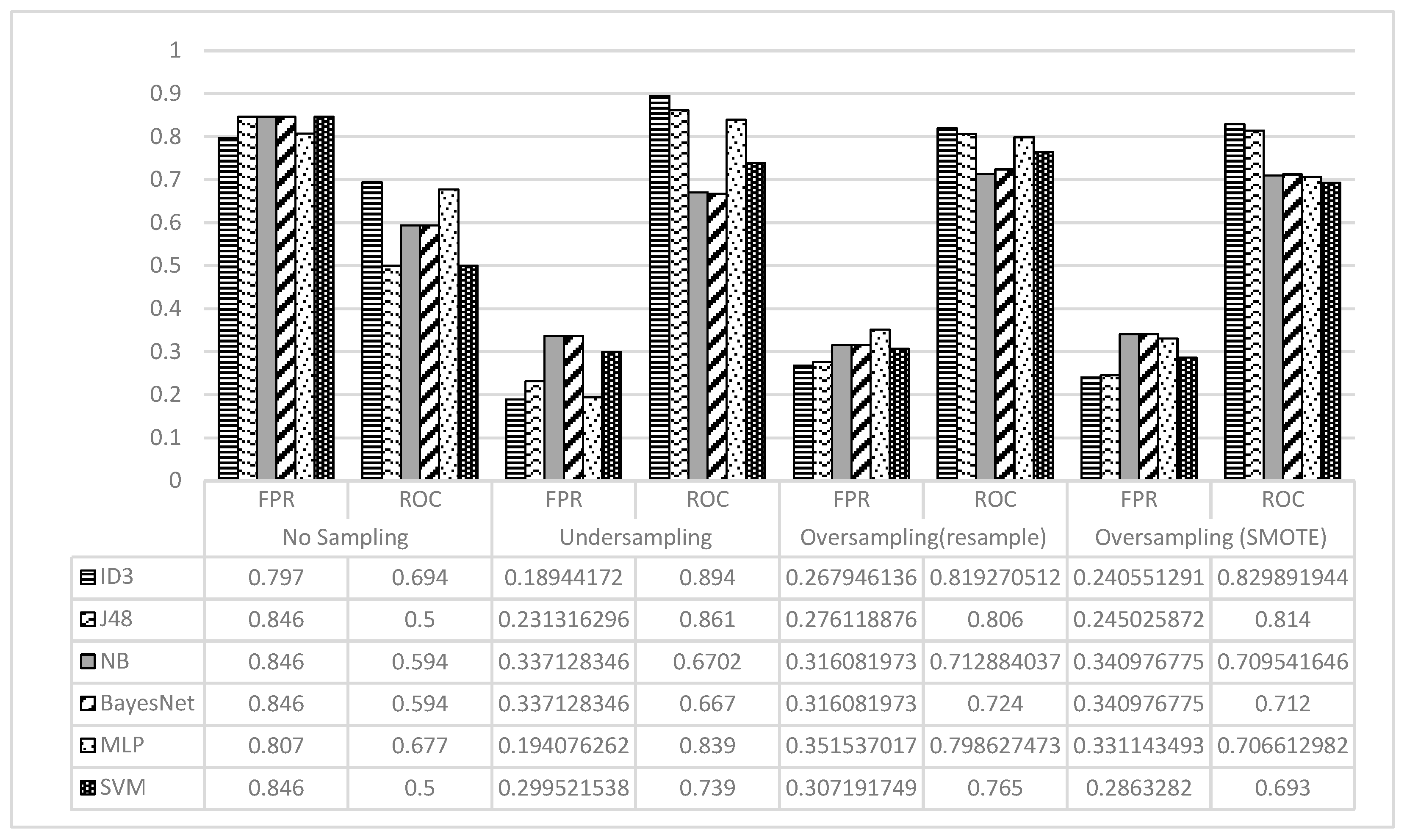
The FPR and ROC values achieved by the classification methods in all scenarios are presented in Figure 7. It is evident that all methods performed poorly in terms of FPR and ROC on the initial data set. The FPR values decrease dramatically after using the sampling techniques. The ROC values also increased considerably for all classification methods. The ID3 was found to be the best classification method in terms of FPR and ROC, followed by the J48 method. The ID3 and J48 achieved their best performances on the undersampled data.
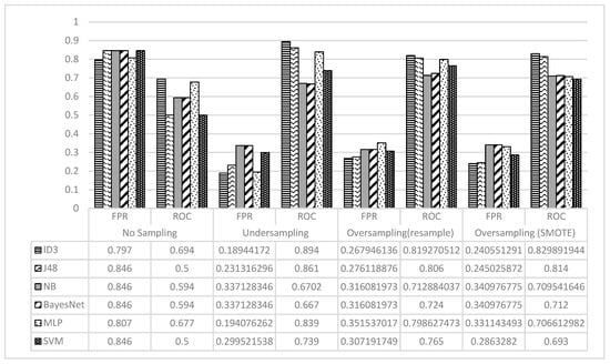
Figure 7.
The FPR and ROC for ID3, NB, and MLP on the Initial, Undersampled, and Oversampled Data.
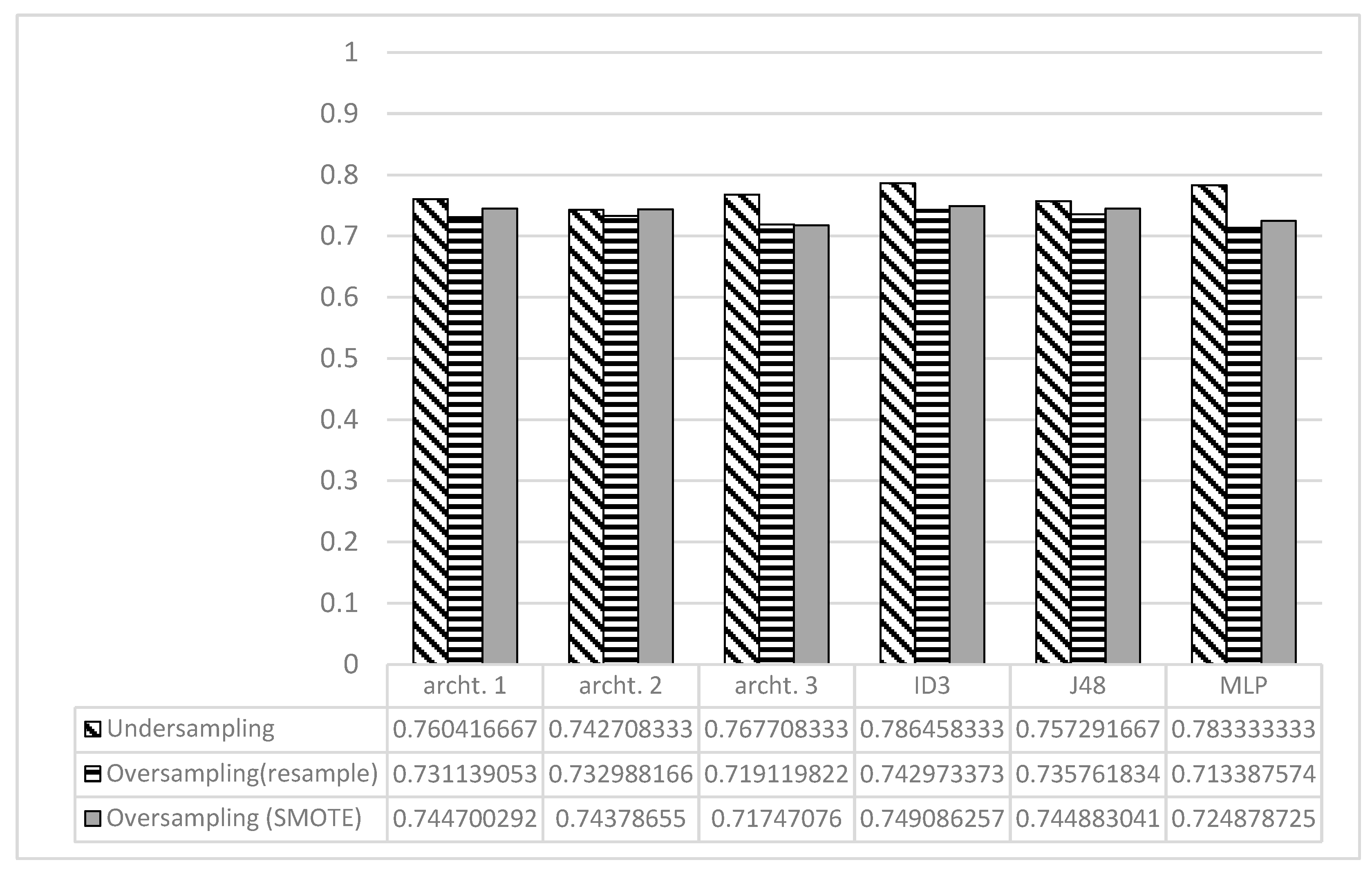
Table 6 shows the performance of the deep learning models built using three different architectures. The results revealed that the best performances were achieved on the undersampled data, with the Archt3 achieving the best results, in terms of accuracy. The results also demonstrated that, for the oversampled data using the resampling technique, the Arch2 provided the best performance, while the Arch1 was the best for the oversample data using SMOTE.
Table 6.
Performance of Archt1, Archt2, and Archt3 on the Undersampled and Oversampled Data.
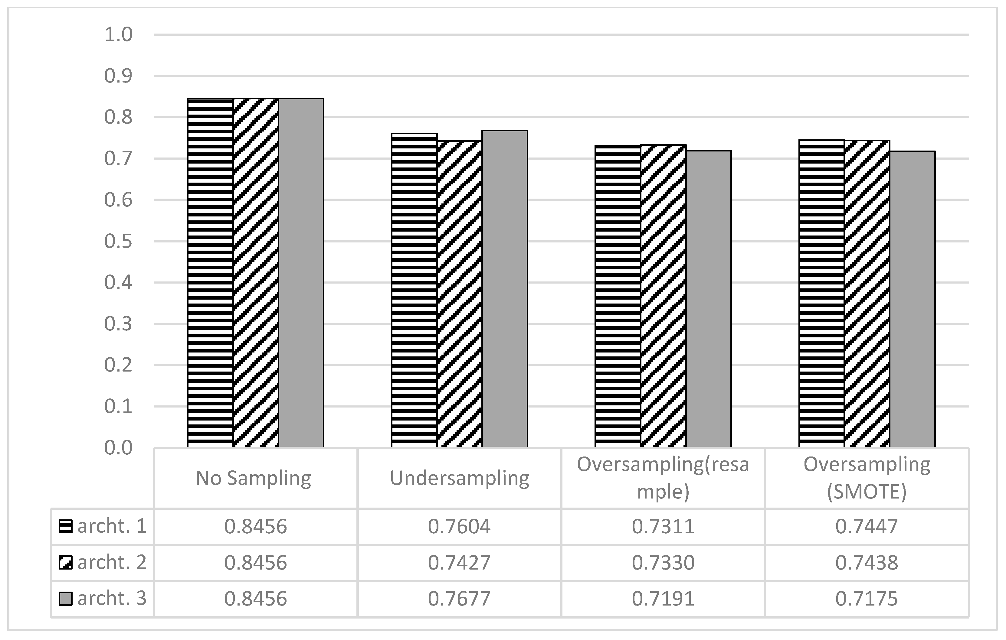
Figure 8 provides a graphical representation of the accuracy achieved by all architectures. Although the highest accuracies were achieved when no sampling techniques were used, the recall values are biased toward the majority class.

Figure 8.
Accuracy Achieved by All DL Architectures.
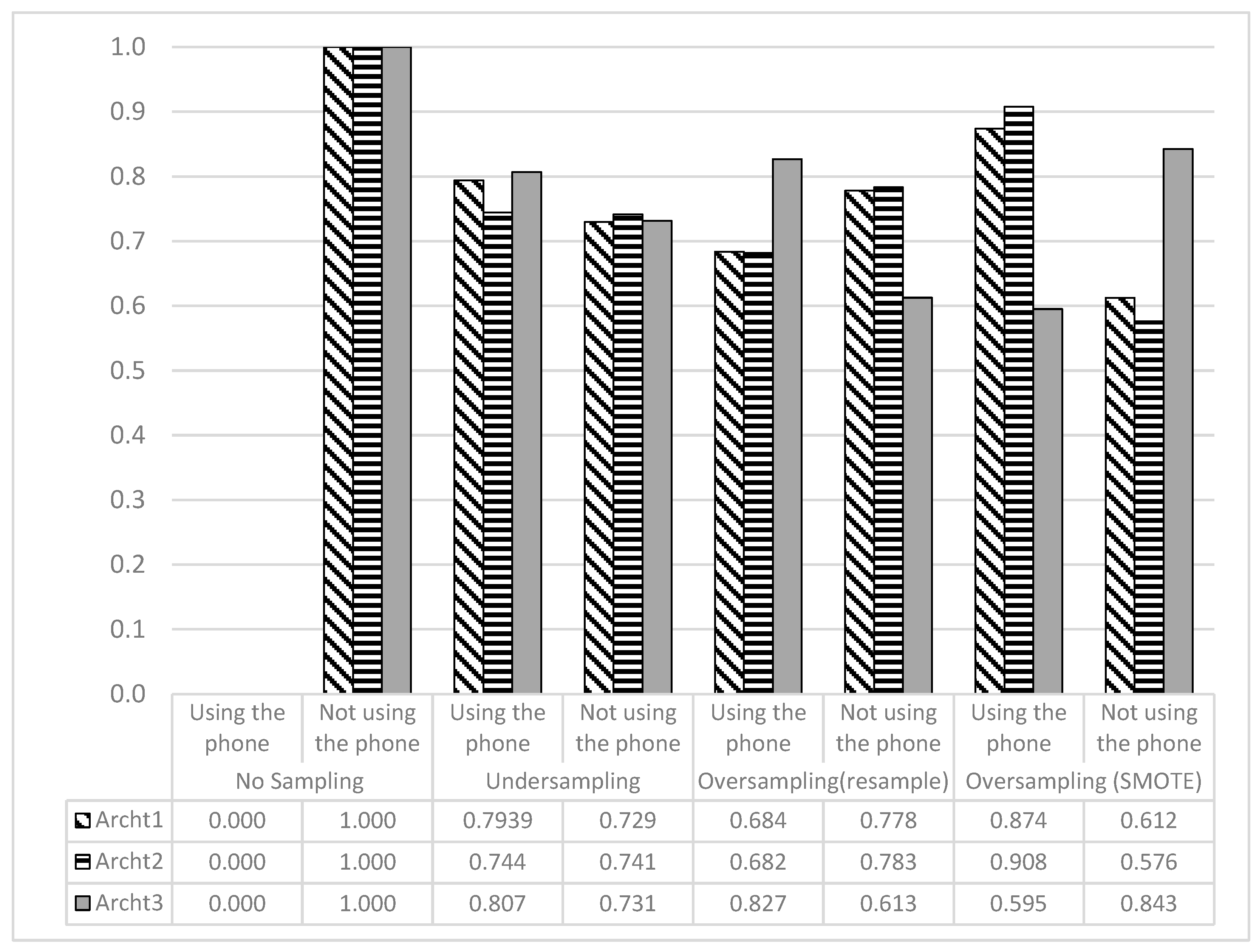
As can clearly be seen from Figure 9, the recall values for the minority class were always zero, but were always one for the majority class. These kinds of models are considered poor for predicting the minority class. On the other hand, the rest of the models that achieved fewer overall accuracies provided balanced recall values for the majority and minority classes.

Figure 9.
Recall Values for Each Class, Generated by All DL Architectures on the Sampled Data.
As Figure 10 indicates, the DL models achieved performances close to those of the best three ML methods, especially on the oversampled data, suggesting that applying the sampling techniques on the unbalanced data prior to run the DL model could be beneficial. This also suggests that the real potential of the DL models requires having larger datasets.
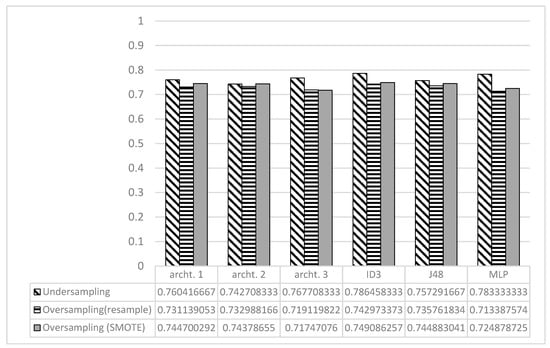
Figure 10.
Accuracy Achieved by ML and DL Models.
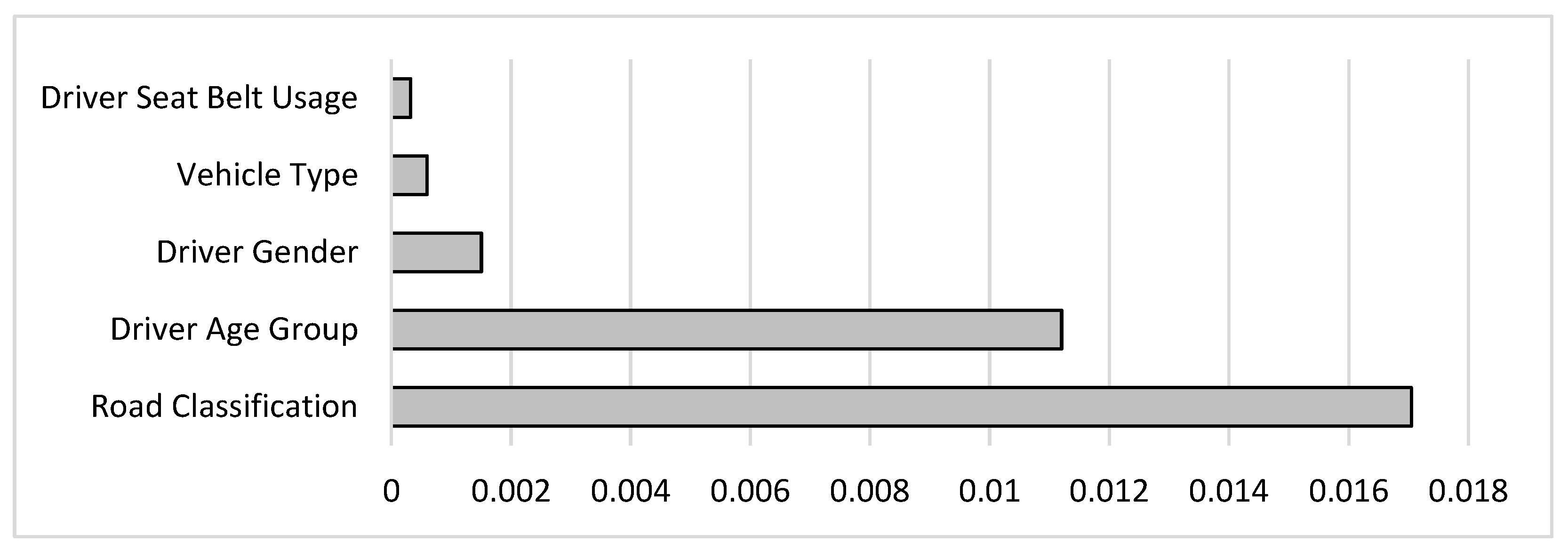
In addition to its capability to predict the tendency of cell phone usage, the ID3 classifier provides a set of rules extracted from the training data in a tree format. Traffic agencies can use such rules to understand the leading factors behind this behavior better, and to develop relevant regulations and laws. To focus on the essential rules, the “InfoGainAttributeEval” attribute evaluator was utilized to reduce the number of attributes by only including the most influential attributes or features. The InfoGainAttributeEval measures the information gained concerning the target variable. The higher the information gain is, the more effect the attribute has on deciding the drivers’ tendency to use the phone. The results showed that the passenger-related attributes had the least significant effect on the target variable compared to the other attributes, and, thus, were removed from the features list. The information gained from the remaining attributes is presented in Figure 11. It can be concluded that road classification has the highest impact on cell phone use, followed by driver’s age group, gender, vehicle type, and, finally, driver’s seatbelt usage.

Figure 11.
Information Gain by “InfoGainAttributeEval” Attribute Evaluator.
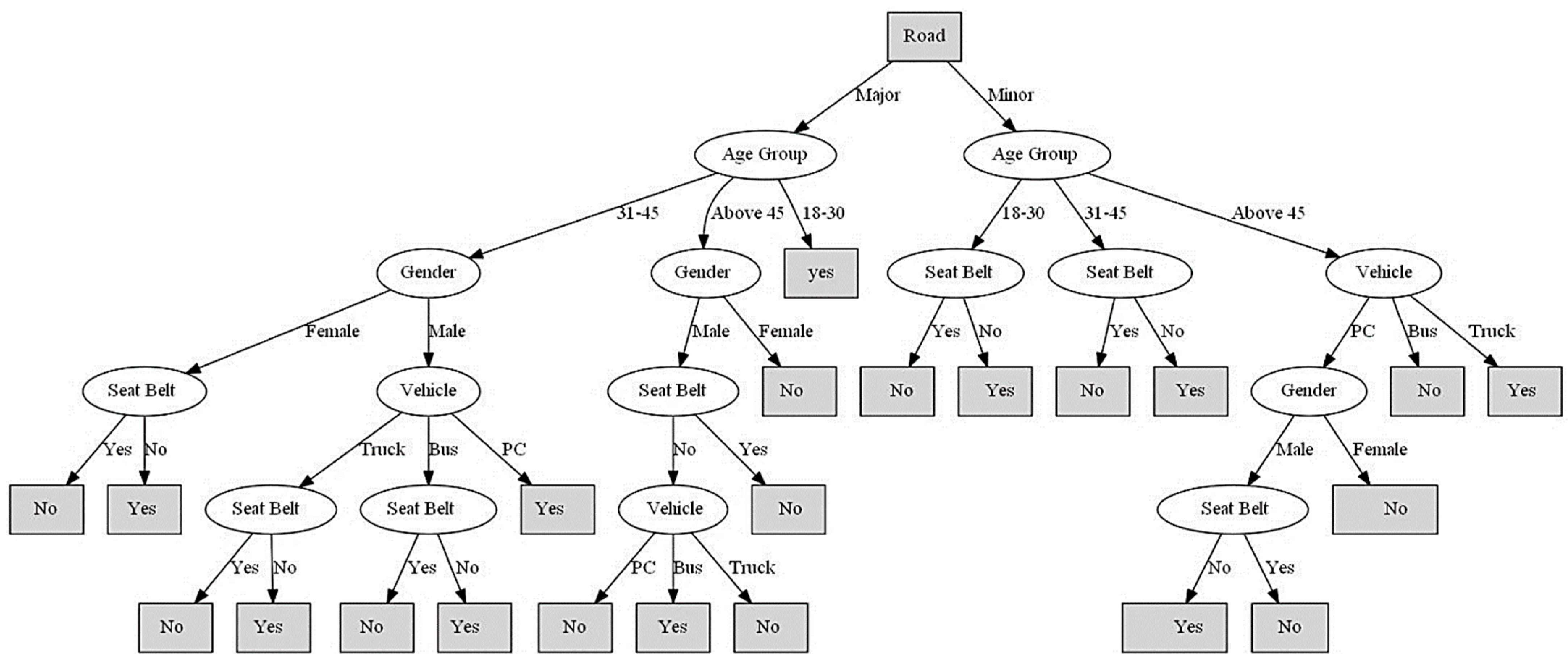
Table 7 shows the rules extracted, and Figure 12 represents the decision tree’s graphical representation. It is worth considering that “Yes” in the leaf nodes means the driver was using his/her cell phone, while “No” means that he/she was not.
Table 7.
Rules Generated by ID3 Algorithm.
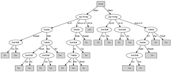
Figure 12.
Decision Tree Generated by the ID3 Algorithm.
Many traffic datasets suffer from unbalanced data, including the phone usage dataset, where there are fewer records of drivers using their phones compared to those who do not. It is worth noting that ML tools are typically designed to perform best on balanced datasets, but this is only sometimes true. Additionally, these tools often prioritize maximizing classification accuracy as their ultimate goal. When these assumptions are made, classifiers tend to ignore the minority class and classify all instances into the majority class, resulting in high classification accuracy. However, these classifiers are not practical. Thus, when dealing with traffic-related data, it is crucial to address the imbalance issue before attempting to apply classification techniques. The classifiers built on balanced datasets are more capable of identifying factors affecting drivers’ compliance with road traffic regulations, such as seatbelt and cell phone use.
The methodology presented in this paper can serve as a technical guide for examining various factors that affect road safety. The systematic approach used in this investigation can be applied in future studies to explore additional aspects that could affect traffic safety and road-user behavior. The findings of this study will assist decision-makers in the field of traffic safety in initiating campaigns aimed at improving driver behavior and enhancing compliance with traffic regulations and rules. The built classifiers can also be used to predict drivers’ compliance in real-time. This capability can be integrated into larger systems to better ensure road safety by authorities.
5. Conclusions
The historical data about drivers is of paramount importance for identifying influential factors contributing to unsafe, reckless behaviors. The distribution of classes in such data is inherently imbalanced. Therefore, handling the imbalanced dataset before analyzing it is essential for accurate results. Handling imbalanced data is specifically important when using ML tools for analysis. Such tools perform very poorly on imbalanced data and provide misleading results. Oversampling and undersampling techniques have proven effective in balancing the datasets. Oversampling aims at increasing the minority class, while undersampling aims at decreasing the majority class. This paper used SMOTE and random resample for oversampling, while random resample was used for undersampling. Six ML techniques (MLP, SVM, NB, BayesNet, J48, and ID3) and three DL architectures (Archt1, Archt2, and Archt3) were then applied to the balanced dataset to assess the performance of the used sampling techniques.
The results showed that the accuracy for the minority class has dramatically improved using the sampling techniques. Among the used classification methods, ID3 provided the best overall accuracy in all scenarios, followed by the J48 and MLP techniques. The DL models also achieved good overall accuracies on both the undersampled and oversampled data. However, the DL models can achieve higher accuracies if the size of the data is bigger. In terms of overall accuracy, the best performance for ID3, J48, and MLP was achieved using the undersampling technique. The same also applies for the DL models. Moreover, the minimum differences between the accuracy of the majority class and the minority class were also achieved when using the undersampling techniques. The gap was larger when using oversampling techniques. The results also showed that the FPR values decreased dramatically after using the sampling techniques, while the ROC values increased for all classification methods. The ID3 was found to be the best classification method in terms of FPR and ROC. The ID3 achieved its best performance on the undersampled data.
The ID3 classifier gives several rules in a tree format, learned from the training data. It can also predict how people will use their cell phones in the future. Traffic agencies can use these guidelines to better understand the main reasons for this behavior and set up the necessary rules and laws. As suggested by the results, the performance of the ML tools can be significantly improved if the dataset is balanced. Oversampling and undersampling are very efficient tools for handling imbalanced datasets. The undersampling technique was found to be the best sampling technique for the used dataset.
Author Contributions
Conceptualization, M.M.T., S.T. and A.H.A.; methodology, M.M.T. and S.T.; software, S.T.; validation, M.M.T. and S.T.; formal analysis, M.M.T., S.T. and A.H.A.; investigation, M.M.T., S.T., A.H.A. and M.A.; resources, M.M.T. and A.H.A.; data curation, S.T. and A.H.A.; writing—original draft preparation, M.M.T., S.T. and A.H.A.; writing—review and editing, M.M.T., S.T., A.H.A. and M.A.; visualization, M.M.T. and S.T.; supervision, M.M.T.; project administration, M.M.T.; funding acquisition, M.M.T., S.T., A.H.A. and M.A. All authors have read and agreed to the published version of the manuscript.
Funding
This research received no external funding.
Institutional Review Board Statement
Not applicable.
Informed Consent Statement
Not applicable.
Data Availability Statement
The data presented in this study are available on request from the first author.
Conflicts of Interest
The authors declare no conflict of interest. The roles in the collection, analysis, interpretation of data, writing of the manuscript, and the decision to publish the results are solely the authors.
References
- World Health Organization. WHO Report 2015: Data Tables; WHO: Geneva, Switzerland, 2015. [Google Scholar]
- World Health Organization. Mobile Phone Use: A Growing Problem of Driver Distraction; WHO: Geneva, Switzerland, 2023; Available online: https://www.who.int/publications/i/item/mobile-phone-use-a-growing-problem-of-driver-distraction (accessed on 1 March 2023).
- Alkheder, S.; Taamneh, M.; Taamneh, S. Severity prediction of traffic accident using an artificial neural network. J. Forecast. 2017, 36, 100–108. [Google Scholar] [CrossRef]
- Dong, C.; Shao, C.; Li, J.; Xiong, Z. An improved deep learning model for traffic crash prediction. J. Adv. Transp. 2018, 2018, 3869106. [Google Scholar] [CrossRef]
- Taamneh, M.; Alkheder, S.; Taamneh, S. Data-mining techniques for traffic accident modeling and prediction in the United Arab Emirates. J. Transp. Saf. Secur. 2017, 9, 146–166. [Google Scholar] [CrossRef]
- Taamneh, M.; Taamneh, S.; Alkheder, S. Clustering-based classification of road traffic accidents using hierarchical clustering and artificial neural networks. Int. J. Inj. Control Saf. Promot. 2017, 24, 388–395. [Google Scholar] [CrossRef] [PubMed]
- Rahim, M.A.; Hassan, H.M. A deep learning based traffic crash severity prediction framework. Accid. Anal. Prev. 2021, 154, 106090. [Google Scholar] [CrossRef]
- Alomari, A.H.; Khedaywi, T.S.; Jadah, A.A.; Marian, A.R.O. Evaluation of Public Transport among University Commuters in Rural Areas. Sustainability 2023, 15, 312. [Google Scholar] [CrossRef]
- Alomari, A.H.; Khedaywi, T.S.; Marian AR, O.; Jadah, A.A. Traffic speed prediction techniques in urban environments. Heliyon 2022, 8, e11847. [Google Scholar] [CrossRef] [PubMed]
- Alomari, A.H.; Abu Lebdeh, E. Smart real-time vehicle detection and tracking system using road surveillance cameras. J. Transp. Eng. Part A Syst. 2022, 148, 04022076. [Google Scholar] [CrossRef]
- Alomari, A.H.; Al-Mistarehi, B.W.; Alnaasan, T.K.; Obeidat, M.S. Utilizing Different Machine Learning Techniques to Examine Speeding Violations. Appl. Sci. 2023, 13, 5113. [Google Scholar] [CrossRef]
- Ali, S.F.; Aslam, A.S.; Awan, M.J.; Yasin, A.; Damaševičius, R. Pose estimation of driver’s head panning based on interpolation and motion vectors under a boosting framework. Appl. Sci. 2021, 11, 11600. [Google Scholar] [CrossRef]
- Alomari, A.H.; Taamneh, M.M. Front-seat seatbelt compliance in Jordan: An observational study. Adv. Transp. Stud. Int. J. 2020, 11, 101–116. [Google Scholar] [CrossRef]
- Raman, S.R.; Ottensmeyer, C.A.; Landry, M.D.; Alfadhli, J.; Procter, S.; Jacob, S.; Hamdan, E.; Bouhaimed, M. Seat-belt use still low in Kuwait: Self-reported driving behaviours among adult drivers. Int. J. Inj. Control Saf. Promot. 2014, 21, 328–337. [Google Scholar] [CrossRef]
- Fiorentini, N.; Losa, M. Handling imbalanced data in road crash severity prediction by machine learning algorithms. Infrastructures 2020, 5, 61. [Google Scholar] [CrossRef]
- Sarkar, S.; Khatedi, N.; Pramanik, A.; Maiti, J. An ensemble learning-based undersampling technique for handling class-imbalance problem. In Proceedings of the ICETIT 2019: Emerging Trends in Information Technology, Delhi, India, 21–22 June 2019; Springer International Publishing: Cham, Switzerland, 2020; pp. 586–595. [Google Scholar]
- Shi, X.; Wong, Y.D.; Li, M.Z.F.; Palanisamy, C.; Chai, C. A feature learning approach based on XGBoost for driving assessment and risk prediction. Accid. Anal. Prev. 2019, 129, 170–179. [Google Scholar] [CrossRef]
- Parsa, A.B.; Taghipour, H.; Derrible, S.; Mohammadian, A.K. Real-time accident detection: Coping with imbalanced data. Accid. Anal. Prev. 2019, 129, 202–210. [Google Scholar] [CrossRef]
- Elamrani Abou Elassad, Z.; Mousannif, H.; Al Moatassime, H. Class-imbalanced crash prediction based on real-time traffic and weather data: A driving simulator study. Traffic Inj. Prev. 2020, 21, 201–208. [Google Scholar] [CrossRef] [PubMed]
- Cai, Q.; Abdel-Aty, M.; Yuan, J.; Lee, J.; Wu, Y. Real-time crash prediction on expressways using deep generative models. Transp. Res. Part C Emerg. Technol. 2020, 117, 102697. [Google Scholar] [CrossRef]
- Peng, Y.; Li, C.; Wang, K.; Gao, Z.; Yu, R. Examining imbalanced classification algorithms in predicting real-time traffic crash risk. Accid. Anal. Prev. 2020, 144, 105610. [Google Scholar] [CrossRef]
- Boonserm, E.; Wiwatwattana, N. Using Machine Learning to Predict Injury Severity of Road Traffic Accidents During New Year Festivals from Thailand’s Open Government Data. In Proceedings of the 2021 9th International Electrical Engineering Congress (iEECON), Pattaya, Thailand, 10–12 March 2021; pp. 464–467. [Google Scholar]
- Mujalli, R.O.; López, G.; Garach, L. Bayes classifiers for imbalanced traffic accidents datasets. Accid. Anal. Prev. 2016, 88, 37–51. [Google Scholar] [CrossRef]
- Morris, C.; Yang, J.J. Effectiveness of resampling methods in coping with imbalanced crash data: Crash type analysis and predictive modeling. Accid. Anal. Prev. 2021, 159, 106240. [Google Scholar] [CrossRef]
- Bedane, T.T.; Assefa, B.G.; Mohapatra, S.K. Preventing Traffic Accidents Through Machine Learning Predictive Models. In Proceedings of the 2021 International Conference on Information and Communication Technology for Development for Africa (ICT4DA), Bahir Dar, Ethiopia, 22–24 November 2021; pp. 36–41. [Google Scholar]
- Jeong, H.; Jang, Y.; Bowman, P.J.; Masoud, N. Classification of motor vehicle crash injury severity: A hybrid approach for imbalanced data. Accid. Anal. Prev. 2018, 120, 250–261. [Google Scholar] [CrossRef] [PubMed]
- Basso, F.; Pezoa, R.; Varas, M.; Villalobos, M. A deep learning approach for real-time crash prediction using vehicle-by-vehicle data. Accid. Anal. Prev. 2021, 162, 106409. [Google Scholar] [CrossRef] [PubMed]
- Schlögl, M.; Stütz, R.; Laaha, G.; Melcher, M. A comparison of statistical learning methods for deriving determining factors of accident occurrence from an imbalanced high resolution dataset. Accid. Anal. Prev. 2019, 127, 134–149. [Google Scholar] [CrossRef] [PubMed]

Disclaimer/Publisher’s Note: The statements, opinions and data contained in all publications are solely those of the individual author(s) and contributor(s) and not of MDPI and/or the editor(s). MDPI and/or the editor(s) disclaim responsibility for any injury to people or property resulting from any ideas, methods, instructions or products referred to in the content. |
© 2023 by the authors. Licensee MDPI, Basel, Switzerland. This article is an open access article distributed under the terms and conditions of the Creative Commons Attribution (CC BY) license (https://creativecommons.org/licenses/by/4.0/).