Article

Optimizing Perishable Product Supply Chain Network Using Hybrid Metaheuristic Algorithms

1
Business School, Hunan University, Changsha 410082, China
2
Business School, Hunan Agricultural University, Changsha 410128, China
*
Authors to whom correspondence should be addressed.
Sustainability 2023, 15(13), 10711; https://doi.org/10.3390/su151310711
Submission received: 29 May 2023 / Revised: 26 June 2023 / Accepted: 5 July 2023 / Published: 7 July 2023

Abstract

:
This paper focuses on optimizing the long- and short-term planning of the perishable product supply chain network (PPSCN). It addresses the integration of strategic location, tactical inventory, and operational routing decisions. Additionally, it takes into consideration the specific characteristics of perishable products, including their shelf life, inventory management, and transportation damages. The main objective is to minimize the overall supply chain cost. To achieve this, a nonlinear mixed integer programming model is developed for the multi-echelon, multi-product, and multi-period location-inventory-routing problem (LIRP) in the PPSCN. Two hybrid metaheuristic algorithms, namely genetic algorithm (GA) and multiple population genetic algorithm (MPGA), are hybridized with variable neighborhood search (VNS) and proposed to solve this NP-hard problem. Moreover, a novel coding method is devised to represent the complex structure of the LIRP problem. The input parameters are tuned using the Taguchi experimental design method, considering the sensitivity of meta-heuristic algorithms to these parameters. Through experiments of various scales, the hybrid MPGA with VNS indicates superior performance, as evidenced by the experimental results. Sensitivity analysis is conducted to examine the influence of key model parameters on the optimal objective, providing valuable management implications. The results clearly validate the efficacy of the proposed model and solution method as a reliable tool for optimizing the design problem of the PPSCN.

1. Introduction

In recent decades, there has been a significant increase in the demand for perishable products in various markets. At the same time, customers in different countries have become more and more concerned about the freshness of these products. However, perishable products, including vegetables, fruits, and milk, are prone to deterioration shortly after production. The global issue of food waste is particularly severe in the United States, with approximately 15% of perishable products spoiling during transportation and sales each year. Additionally, perishable product sales constitute half of the overall retail industry [1], while about 10% of perishable goods are wasted before being purchased by customers [2,3]. In China, over 25% of fruits and vegetables deteriorate during transportation, storage, and sales [4,5]. The rates of fresh produce deterioration in inventory and transportation in China are approximately 15% for fruits, 8% for vegetables, and 10% for meat and aquatic products [5]. To address these challenges, it is crucial to implement effective inventory control, optimize transportation routes, and enhance operational efficiency within the perishable product supply chain.
The period between the manufacturing date and the final delivery to the end customers holds significant importance for both producers and traders of perishable products. The vulnerability of perishable items to damage and spoilage introduces specific constraints on various aspects of the supply chain, including facility location, distribution planning, inventory management, and routing arrangements. Undoubtedly, considering the unique nature of perishable goods, this issue becomes even more critical. Therefore, there is an urgent requirement to develop a specialized and comprehensive optimal supply chain network model that caters to the specific needs of perishable products [6,7]. Additionally, ensuring cost effectiveness poses a significant challenge in the management of goods with a limited shelf life.
To minimize the economic cost of the PPSCN, this study develops a novel model that considers the perishable characteristics of the products. The LIRP model involves the integrated optimization of facility location, inventory management, and routing arrangement within the supply chain network. This integration tackles the logistics LIRP, which poses a comprehensive optimization challenge for the entire logistics system [8]. The purpose of this study is to provide an optimized solution for supply chain managers or practitioners, empowering them to efficiently manage the PPSCN and achieve cost effectiveness.
Since the LIRP is characterized by its size, complexity, and nonlinear nature, it is not always feasible to obtain an optimal solution using exact methods. Nowadays, metaheuristic algorithms have been commonly used globally for their simple structure and other advantageous qualities, such as adaptability and flexibility [9]. GA has the advantage of providing feasible solutions that are close to optimal, even in scenarios where the problem’s constraints or objective function are non-continuous and do not necessitate a linear formulation.
The proposed metaheuristic algorithms in this paper comprise HGA-VNS and HMPGA-VNS, where GA and MPGA are, respectively, hybridized with VNS. Hybrid metaheuristic algorithms leverage the strengths of different algorithms while mitigating their weaknesses [10,11]. GA and MPGA contribute global information and search guidance to VNS, while VNS enhances the search diversity and global search capability of GA and MPGA.
The field of PPSCN has gained significant attention in recent years. A predominant research focus is designing a supply chain network for perishable goods while addressing the uncertainties associated with their perishability. This paper’s modeling and solution approach is inspired by previous research conducted in the field of PPSCN. In the subsequent section, we provide a concise overview of these studies.
Before delving into the review of previous studies on the LIRP, it is important to first examine the studies that address two key categories of decisions in supply chain management.
The location–inventory problem (LIP) involves determining optimal facility locations and corresponding inventory levels within the SCN to meet customer demand while minimizing costs. Researchers have examined various types of this problem to address real-world scenarios in the PPSCN [12,13,14,15,16]. For instance, Dai, Aqlan, Zheng and Gao [3] incorporated a LIP into the PPSCN considering fuzzy capacity and carbon emission constraints. They proposed two heuristic approaches, namely the hybrid genetic algorithm (HGA) and the hybrid harmony search (HHS), to solve the model. Numerical experiments demonstrated that HHS obtained higher-quality solutions compared to HGA, although HGA exhibited faster computational performance.
The inventory-routing problem (IRP) refers to optimization of inventory and routing plans within a supply chain to improve logistics efficiency and cost effectiveness. When it comes to perishable products, it is crucial to develop optimal joint policies [17,18,19,20]. Azadeh et al. [21] proposed an IRP model that incorporates transshipment and a single perishable product. They also devised a method based on GA to address this problem. Rohmer et al. [22] presented a two-echelon IRP for perishable products and utilized an adaptive large neighborhood search metaheuristic combined with a simplified formula to solve the problem. They compared three variations of the heuristic on randomly generated instances.
In the location-routing problem (LRP), the objective is to determine the optimal location and capacity of a logistics distribution center (DC). Subsequently, an optimal distribution route and vehicle arrangement are designed to enhance operational efficiency and minimize logistics costs. Wu et al. [23] introduced a three-echelon LRP that considers time windows and time budget restrictions for perishable food products to high-speed railways. A hybrid cross-entropy algorithm was applied to solve a case study conducted in China. In the pharmaceutical industry, Zhu and Ursavas [24] proposed an LRP that incorporates time windows and direct delivery constraints.
Having explored the fundamental concepts, we are now ready to delve into the main subject. Several scholars have already conducted research on the logistics LIRP specifically focused on perishable products. Chen et al. [25] conducted an analysis on a two-stage LIRP with time window constraints specifically for food products. They utilized a hybrid heuristic algorithm to solve a mixed-integer programming model. In a similar vein, Zandkarimkhani et al. [26] proposed a bi-objective mixed-integer linear programming (MILP) model to address a perishable pharmaceutical supply chain network problem, aiming to minimize total cost and lost demand amount. Rafie-Majd et al. [27] presented a mathematical model for the LIRP involving multi-period and multi-perishable products considering stochastic demands from retailers. Their study incorporated suppliers, DCs, and retailers while accounting for factors such as vehicle schedules, fuel consumption, driver cost, and product waste cost. The Lagrange relaxation method and a heuristic algorithm were employed to solve the model. Hiassat et al. [28] developed a GA and a novel chromosome representation approach to tackle the LIRP for a single perishable product in a single period. Partovi et al. [29] proposed a revised solution method for a bi-level LRP in a two-echelon supply chain with perishable products considering uncertain demand and capacity constraints. Their model incorporated scenario-based programming and employed multi-choice goal programming to minimize deviations from ideal solutions. Aghighi et al. [30] devised a two-phase hybrid mathematical model for the LIRP concerning perishable products. In the first phase, they formulated the LRP considering stochastic demands and travel time. The second phase involved modeling the inventory control problem using a queue system based on the established locations and routes. The model was solved using an improved GA. Biuki et al. [31] introduced the three dimensions of sustainable development into the supply chain network and examined the LIRP for PPSCN. They constructed a two-phase optimization model and combined GA and particle swarm optimization (PSO) algorithms to solve it. Lastly, Liu et al. [5] addressed the challenges of sustainable PPSCN in emerging markets. They developed a comprehensive model that integrates location, inventory, and routing factors, aiming to minimize economic costs and carbon emissions while maximizing product freshness.
As mentioned previously, the existing research on LIRP for PPSCN encompasses various problem types such as deterministic, stochastic, single-period, multi-period, single-product, multi-product, and others. These studies have examined the impact of perishable products on inventory and transportation processes, including damage, specific shelf life, and occurrences during these processes. Some scholars have focused on one or two of these elements. Table 1 provides a comparison of our work and the related literature.
The main innovations and contributions of this study that differentiate it from existing ones are the following:
  • Formulating a novel LIRP model that addresses the design of a multi-period, multi-product PPSCN while simultaneously considering damage in the inventory and transportation processes, as well as specific shelf life;
  • Developing two hybrid metaheuristic algorithms: hybrid GA and VNS (HGA-VNS) and hybrid MPGA and VNS (HMP-GA-VNS) to search for optimal solutions;
  • Designing a new chromosome representation for the unique structure of the problem;
  • Employing the Taguchi experimental design method and conducting means and analysis of variance to assess the effectiveness of the developed hybrid metaheuristic algorithms;
  • Conducting sensitivity analysis to validate the proposed model.
The paper is organized as follows: Section 2 presents the problem and the mathematical model. Section 3 provides an overview of the proposed solution methods. Section 4 includes the Taguchi experimental design method, computational results, sensitivity analyses, and managerial insights. Lastly, in Section 5, conclusions, limitations, and future works are provided.

2. Problem Description

Given the perishable nature of products and the importance of managing their logistics, it is crucial to design an appropriate SCN and focus on the flow of products within the network’s nodes and arcs. Hence, supply chain managers need to consider both the overall cost of the system and the duration of product perishability. This study incorporates the perishable characteristics of the products into the model, known as LIRP, and proposes an integrated approach to minimize the total cost. Specifically, we investigate an SCN that comprises manufacturers, DCs, and retailers, considering multiple periods and multiple perishable products.
In this study, the locations of the retailers and manufacturers are predetermined, while those of the DCs are determined by the model. In each period, DCs receive products from manufacturers and subsequently distribute them to retailers by optimized routing and a fleet of heterogeneous vehicles. Wastage may occur during both the inventory process and transportation process, encompassing transportation from manufacturers to DCs and from DCs to retailers. Products exhibit variations in terms of shelf life, thus requiring DCs to ensure that the products delivered to retailers are within their designated shelf life. To minimize product waste, DCs adopt a First-In-First-Out (FIFO) approach [29]. The proposed model aims to reduce the overall network cost by addressing the following key challenges: (1) determining the optimal quantity and locations of DCs, (2) allocating the retailers to the identified DCs for any given product and period, and (3) determining the most efficient vehicle routes from DCs to retailers for any given period.

2.1. Assumptions

This study is based on the following assumptions:
  • Each retailer is served by one vehicle for one perishable product at any period.
  • The demands of retailers are independent and follow specific probability distributions.
  • Each product in the system has a predetermined shelf life.
  • The number of DCs and their capacities are limited.
  • The vehicle routing problem is specifically defined between the DCs and retailers.
  • The number and capacity of vehicles are predetermined.
  • Shortage considerations are not included.

2.2. Notation

Sets and index:
i Manufacturer   index   i I
j DC   index   j J
k Retailer   index   k K
v Vehicle   index   v V
p Perishable   product   index   p P
t Period   index   t T
Parameters
f i 1 The   fixed   operating   cos ts   for   manufacturer   i
p c i p The   unit   production   cos t   of   perishable   product   p at manufacturer i
t c i j p 1 The   unit   transportation   cos t   of   perishable   product   p   from   manufacturer   i   to   DC   j
m i p t c a p The   capacity   of   manufacturer   i
s i j 1 The   distance   from   manufacturer   i   to   DC   j
f j 2 The   fixed   operating   cos t   for   DC   j
h c j p The   inventory   cos t   of   perishable   product   p   at   DC   j
t c l n v p 2 The   transportation   cos t   of   perishable   product   p   from   DC   j to   retailer   k
α The waste rate during the transportation process in all systems
s l n 2 The   distance   from   node   l   to   node   n
r c p The   waste   cos t   for   perishable   product   p
d k p t The   demand   of   perishable   product   p at   retailer   k d u r i n g   period   t
v v p c a p The   capacity   of   vehicle   v
τ p The   shelf   life   of   perishable   product   p
MA sufficiently large number
Decision variables
x j 1 ,   if   DC   j is operated; 0, otherwise
y i j p t 1 1 ,   if   DC   j   is   supplied   by   manufacturer   i   for   perishable   product   p   during   period   t ; 0, otherwise
y j k p t 2 1 ,   if   retailer   k     is   supplied   by   DC   j   for   product   p   during   period   t ; 0, otherwise
y j k v p t 3 1 ,   if   the   order   quantity   from   DC   j   to   retailer   k   is   delivered   by   vehicle   v   during   period   t ; 0, otherwise
z l n v p t 1 ,   if   link   l n   is   a   part   of   the   vehicle   route   for   delivering   perishable   product   p   by   vehicle   v   during   period   t ; 0, otherwise
u j k m t 1, if perishable product p is procured during period m and delivered out from DC j during period t; 0, otherwise
q i p t 1 Production   quantity   of   perishable   product   p   at   manufacturer   i   during   period   t
w i j p t 1 Purchasing   quantity   of   perishable   product   p   by   DC   j   from   manufacturer   i   during   period   t
w j p t 2 Inventory   quantity   of   perishable   product   p   at   DC   j   during   period   t
w j p t 3 Waste   quantity   of   perishable   product   p   at   DC   j   during   period   t
w j p t 4 Total   delivered   quantity   of   perishable   product   p   by   DC   j   during   period   t
w j p m t 5 Quantity   of   perishable   product   p   procured   during   period   m   and   delivered   out   from   DC   j   during   period   t
w j v p t 6 Quantity   of   perishable   product   picked   up   from   DC   j   by   vehicle   v   at   period   t
w l n v p t 7 Load   quantity   of   perishable   product   p   transported   by   vehicle   v   from   node   l   to   node   n   during   period   t
w j k p t 8 Allocation   quantity   of   perishable   product   p   from   DC   j   to   retailer   k   during   period   t
w j k v p t 9 Delivered   quantity   of   perishable   product   p   by   vehicle   v   from   DC   j   to   retailer   k   during   period   t
θ l v p t Auxiliary non-negative variable used for subtour elimination

2.3. Mathematical Model

According to the problem descriptions, assumptions, and notations, this study formulates the LIRP for a multi-period, multi-product PPSCN as a mixed-integer nonlinear programming (MINLP) model. The formulation contains five costs: fixed cost, production cost, transportation cost, inventory cost, and waste cost.
m i n f = i I f i 1 + j J f j 2 x j The   fixed   cost   of   manufacturers   and   operated   DCs + i I p P t T p c i p q i p t 1 The   production   cost + ( i I j J p P t T t c i j p s i j 1 w i j p t 1 y i j p t 1 + l J K n J K v V p P t T t c l n v p 2 s l n 2 w l n v p t 7 z l n v p t ) ( T h e   t r a n s p o r t a t i o n   c o s t ) + j J p P t T h c j p w j p t 2 T h e   i n v e n t o r y   c o s t + ( j J v V p P t T α · r c j p w i j p t 1 y i j p t 1 + j J p P t T r c j p w j p t 3 + j J v V p P t T α · r c j p w j v p t 6 T h e   w a s t e   c o s t ,
subject to
i I y i j p t 1 x j j , p , t ,
j J y j k p t 2 = 1 , k , p , t ,
y j k p t 2 x j , j , k , p , t ,
y j k p t 2 = v V y j k v p t 3 , j , k , p , t ,
j J k K z j k v p t = 1 , v , p , t ,
k K j J z k j v p t = 1 , v , p , t ,
l J K v V z l k v p t = 1 , k , p , t ,
l J K z l k v p t l J K z k l v p t = 0 , k , v , p , t ,
θ l v p t θ n v p t + M z l n v p t M 1 l J K , n K , v , p , t , l n ,
z j k v p t y j k p t 2 , j , k , v , p , t       z k j v p t y j k p t 2 , j , k , v , p , t       z l j v p t = 0 , l J , j , l j , v , p , t         z l k v p t 0 , l K , k K , l k , v , p , t     ,
( 1 α ) q i p t 1 = j J w i j p t 1 y i j p t 1 , i , p , t ,
q i p t 1 m i p t c a p i , p , t ,
w j p t 2 = i I w i j p t 1 y i j p t 1 w j p t 3 w j p t 4 j , p , t , t = 1           w j p t 1 2 + i I w i j p t 1 y i j p t 1 w j p t 3 w j p t 4 j , p , t , t 2         ,
w k p t 3 = i w i j p t τ p 1 y i j p t τ p 1 g = t τ p t 1 w j p t τ p g 5 u j p t τ p g         j , p , t , t > τ p           0         j , p , t , t τ p                 ,
w j p t 4 = v V w j v p t 6 j , p , t ,
w j p t 4 = m = t τ p t w j p m t 5 u j p m t         j , p , t , t > τ p m = 1 t w j p m t 5 u j p m t         j , p , t , t τ p ,
u j p m t u j p m + 1 t j , p , m , t ,
w j p m + 1 t 5 1 u j p m + 1 t     h = 1 m i w i j p h 1 y i j p h 1 , g = h t w j k p g 8 y j k p g 2 w j p h + τ p 3 k w j k p g 8 y j k p g 2 + 1       j , p , m , t , m + τ p | T | w j p m + 1 t 5 1 u j p m + 1 t     h = 1 m i w i j p h 1 y i j p h 1 , g = h t w j k p g 8 y j k p g 2 k w j k p g 8 y j k p g 2 + 1       j , p , m , t , m + τ p | T | ,
( 1 α ) w j v p t 6 = k K w j k v p t 9 y j k v p t 3 j , v , p , t ,
w j v p t 6 v v p c a p j , v , p , t ,
w j v p t 6 = w j k v p t 7 j , k , v , p , t ,
l J K z l k v p t l J K w l k v p t 7 w j k v p t 9 l J K w k l v p t 7 = 0 k , v , p , t ,
w k j v p t 7 = 0 j , k , v , p , t ,
w j k p t 8 y j k p t 2 = v V w j k v p t 9 y j k v p t 3 j , k , p , t ,
j J v V w j k v p t 9 y j k v p t 3 = d k p t k , p , t ,
m = t T w j p t m 5 u j p t m i I w i j p t 1 y i j p t 1 j , p , t ,
i I t T w i j p t 1 y i j p t 1 = k K t T w j k p t 8 y j k p t 2 + t = T T w j p t 2 + t T w j p t 3 j , p ,
i I w i j p t 1 y i j p t 1 k K w j k p t 8 y j k p t 2 j , p , t = 1 i I w i j p t 1 y i j p t 1 w j p t 2 w j p t 3 k K w j k p t 8 y j k p t 2 j , p , t 2 ,
x j , y i j p t 1 , y j k p t 2 , y j k v p t 3 , u j k m t , z l n v p t 0,1 ,
q i j p t 1 , w i j v p t 1 , w j p t 2 , w j p t 3 , w j p t 4 , w j p m t 5 , w j v p t 6 , w l n v p t 7 , w j k p t 8 , w j k v p t 9 0 .
The objective Function (1) aims to minimize the total cost of the supply chain. Constraint (2) ensures that an operated DC is served by at least one manufacturer. Constraints (3) and (4) require that each retailer is served by an operated DC. Constraint (5) reveals the relationship between service and delivery vehicles from DCs to retailers. Constraints (6) and (7) ensure that when a vehicle leaves the DCs for a retailer, it eventually returns to the starting point. Constraint (8) guarantees that each retailer is served by only one vehicle for each product in each period. Constraint (9) implies that whenever a vehicle arrives at a retailer location, it must leave again. Constraint (10) is adopted in the proposed model for subtour elimination. Constraint (11) specifies that all arcs must comply with the service relationship between the DC and the retailer. Constraint (12) calculates the production quantity of each product for the manufacturer in each period. Constraint (13) specifies the capacity level of the manufacturer. Constraints (14) and (15) indicate the inventory and waste quantity at the DCs. Constraint (16) ensures that the delivery quantity of the DC is equal to the total quantity of vehicles picked up. Constraint (17) requires that perishable products delivered to retailers remain within their shelf lives. Constraints (18) and (19) enforce the First-In-First-Out (FIFO) policy for perishable products at the DCs. Constraint (20) states that the quantity of perishable products picked up by each vehicle at the DC must be equal to the total quantity delivered by the served retailer. Constraint (21) indicates that the pickup quantity of each vehicle cannot exceed the capacity limitation. Constraints (22)–(24) calculate the load quantity of vehicles in each arc segment. Constraints (25) and (26) specify that vehicles deliver perishable products according to retailer demand. Constraint (27) restricts the delivered quantity of perishable products in the DC to not exceed the purchase quantity. Constraint (28) ensures the flow balance of the DC throughout the entire planning horizon. Constraint (29) calculates the purchase quantity of the DC in each period. Constraints (30) and (31) determine the type and range of decision variables.

3. Solution Algorithms

3.1. Key Element Design of Hybrid Metaheuristic Algorithms

To ensure the effective operation of GA approaches, several essential components need to be considered. These components include an initial population that generates chromosome representations, genetic operators such as crossover and mutation, and mechanisms to handle infeasible solutions. Each of these components are described in detail below.

3.1.1. Chromosome Representation

Each chromosome in the GA contains important information regarding various aspects, including the location of DCs, the suppliers responsible for servicing the DCs, the assignment of DCs to retailers, and the scheduling and routing plan for vehicles from the DCs to retailers. In Figure 1, an example of a chromosome string is presented, representing a scenario involving four suppliers, three DCs, seven retailers, four vehicles with different capacities, two perishable products, and two periods. Each chromosome is divided into four distinct strings, each representing a specific aspect of the solution.
The information encoded in each of the four strings of the chromosome is described below (refer to Figure 1 for visualization).
The first string (Figure 1a) represents the manufacturers-to-DC service decision for each perishable product and period. Each gene value indicates the number of operating DCs served by a specific manufacturer for a perishable product and period. For instance, in Period 1 for Perishable 1, Manufacturer 1 serves DC 3, while Manufacturer 2 serves DC 2.
The second string (Figure 1b) represents the total number of retailers served by each DC for a specific perishable product and period. The gene value indicates the number of retailers served by an operated DC. For example, in Period 1 for Perishable 1, DC 1 is not operating, DC 2 serves three retailers, and DC 3 serves four retailers.
The third string (Figure 1c) represents the allocation of vehicles to DCs. Each gene represents the number of the DC, and the gene values are filled randomly with the number of vehicles. DCs that are not in operation are assigned the value zero. In Figure 1c, for Perishable 1 in Period 1, Vehicle 8 is allocated to DC 2, and Vehicle 9 is allocated to DC 3.
The fourth string (Figure 1d) indicates the allocation of vehicles(blue) to retailers for the purpose of routing. Retailers are assigned sequential numbers starting from 1, while vehicles are numbered consecutively, starting from the last retailer. By combining Figure 1c and Figure 1d, the route for Vehicle 8 is DC2-3-2-6-DC2, and the route for Vehicle 9 is DC3-4-1-5-7-DC3. If two vehicles are adjacent, the leading vehicle is considered idle. For example, in Period 2 for Perishable 2, Vehicle 10 is idle (Figure 1d).

3.1.2. Crossover

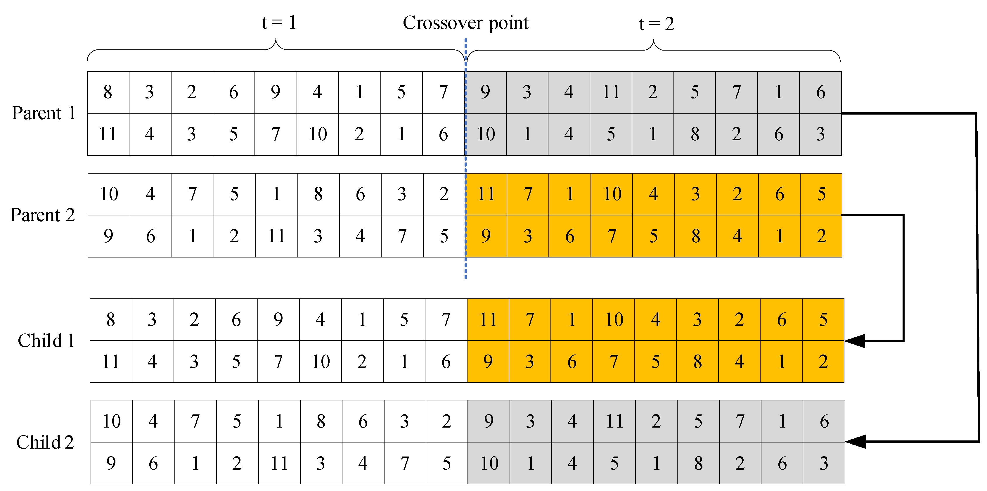
The crossover operator is essential in enhancing the search performance of the GA. It involves three steps:
(1)
Single-point crossover is employed in this study. Specifically, crossovers are applied to String II of the chromosome. Following the approach proposed by Hiassat et al. [28], the crossover points are selected from a valid crossover set, which consists of boundary points between each period.
(2)
A pair of chromosomes is randomly chosen from the set.
(3)
Segmentation is performed, and the right-hand side of the chromosomes is exchanged at the randomly selected location point.
Figure 2 provides an illustrative example of the crossover operator.

3.1.3. Mutation

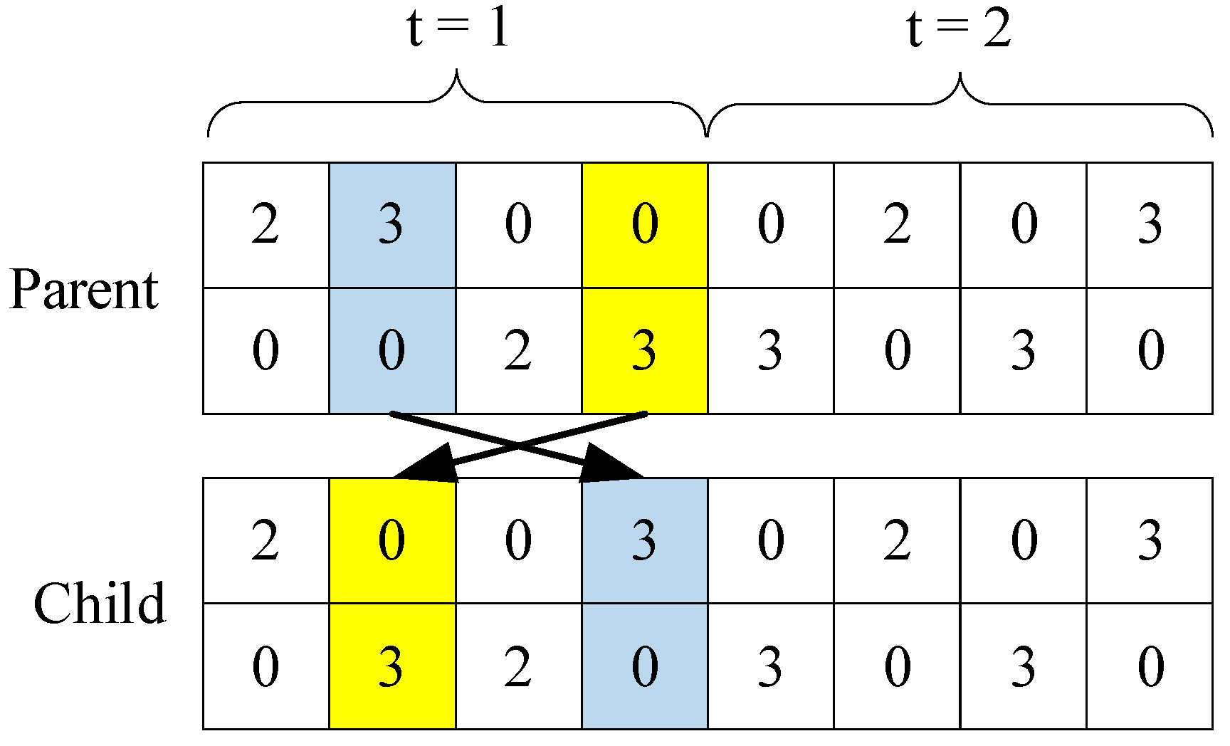
The mutation operator plays a crucial role in expanding the search space of the solution and preventing the GA from being trapped in a local optimum. In this study, mutations are specifically applied to String III of the chromosome, which represents the total number of retailers served by the DCs. The arrangement of vehicles and retailers is carefully structured to ensure the availability of optimal solutions (as depicted in Figure 3).

3.1.4. Infeasible Solution Repair Mechanisms

In metaheuristic algorithms, every chromosome is required to represent a potential solution. However, following the crossover and mutation operations, certain generated chromosomes may no longer adhere to the given constraints, rendering them infeasible. Consequently, these chromosomes need to be repaired to regain their viability within the problem’s limitations.

3.2. Variable Neighborhood Search Algorithm

The VNS algorithm was initially introduced by Mladenovi et al. [32]. It employs a dynamic adjustment of the neighborhood structure during the search process, with the goal of finding optimal solutions that balance between focused local area search and diverse exploration of larger areas. VNS is particularly effective in tackling local optimization problems associated with NP-hard problems, including constrained optimization problems [33,34]. Algorithm 1 presents the pseudocode of VNS.
Algorithm 1: Pseudocode of VNS
1Initialization
  Parameters: maximum iterations of VNS (Maxiter), neighbourhood structures size N l l = 1 , l m a x
  Receive/generate population with size P and assess them
  Pick up the best solution as initial solution X *
2For iter     Maxiter do
3  For  N l   l m a x    do
4   X = shaking ( X * , N l )
5  X″ = local search ( X )
6    If f X X *
7             X * X
8    l = 1;
9    Else
10    l = l + 1;
11    End if
12   End for
13  End for
14  Report the best solution;
15  End

3.3. HGA-VNS Algorithm

The GA is a metaheuristic algorithm that emulates the genetic and evolutionary processes observed in biological evolution. It iteratively evolves and searches for the optimal solution to a problem. GA possesses several advantages, including robust search capabilities, adaptability, parallelization, and straightforward implementation. As a result, it is highly effective in tackling NP-hard problems [35]. The HGA-VNS algorithm leverages the robust search capability of GA and the local search technique of VNS to achieve optimal results. Algorithm 2 provides the pseudocode for the HGA-VNS approach.
Algorithm 2: Pseudocode of HGA-VNS
Step 1:  Initialization
  Step 1.1: Set parameters: population size ( P ), maximum iterations ( M a x _ i t e r ), crossover rate ( P c ), mutation rate ( P m )
  Step 1.2: Generate individuals using the coding mechanism to form the initial population
Step 2: Calculation of individual fitness values ()
Step 3: Select operation ()
Step 4: Crossover operation ()
Step 5: Mutation operation ()
Step 6: Repairing operation ()
Step 7: VNS local search ()
Step 8: Repeat steps 2 to 7 until the maximum iterations of the GA are reached
Step 9: Final solution ()

3.4. HMPGA-VNS Algorithm

The MPGA is an extended version of GA that enhances its capabilities. MPGA incorporates multiple independent populations that operate in parallel to perform search and optimization. Each population comprises multiple individuals that perform genetic operations, including selection, crossover, mutation, and fitness evaluation. Specific communication mechanisms, such as information sharing and individual migration, are implemented to facilitate information exchange and maintain diversity among the populations. This enables MPGA to conduct a more comprehensive and efficient search. MPGA effectively tackles challenges encountered in single-population GA, such as convergence and being trapped in local optima. The computational aspects of MPGA are summarized in the following section.
Step 1: Initialize a population and divide it into n subpopulations.
Step 2: Independently perform selection, crossover, mutation, and evaluation operations on each subpopulation.
Step 3: Conduct migration operations among the subpopulations.
Step 4: Repeat steps 2 to 3 until the termination criteria are satisfied.
Step 5: Merge each subpopulation to form a population.
Step 6: Select the optimal individual from the population.
The MPGA has been successfully applied to solve NP-hard global optimization problems such as transportation scheduling, parallel machine scheduling, dynamic facility layout, and multi-energy complementary system optimization [36,37,38,39]. The HMPGA-VNS employs a distinct strategy where the population is divided into P/SP subpopulations that perform independent genetic operations. After generating offspring subpopulations, a subset of the top-performing individuals is randomly migrated to other subpopulations to promote diversity. Subsequently, the subpopulations are merged. The integration of VNS as a local search technique facilitates the improvement of individuals within the population and the achievement of optimal solutions at each iteration. Algorithm 3 presents the pseudocode for the HMPGA-VNS algorithm.
Algorithm 3: Pseudocode of HMPGA-VNS
Step 1:  Initialization
  Step 1.1: Set parameters: population size ( P ), subpopulation size ( S P ), maximum iterations ( M a x _ i t e r ), crossover rate ( P c ), mutation rate ( P m ), migration period ( M p ), migration size ( M s ).
  Step 1.2: Generate individuals according to the coding mechanism to form the initial population, which is then divided into P/SP subpopulations.
Step 2: Evolutionary operations for each subpopulation (same as GA, but operated independently):
  Step 2.1: Perform selection operation within each subpopulation ().
  Step 2.2: Conduct crossover operation within each subpopulation ().
  Step 2.3: Perform mutation operation within each subpopulation ().
Step 3: Perform repairing operation within each subpopulation ().
Step 4: Calculate individual fitness values within each subpopulation ().
 Select individuals with better fitness values as representatives of each subpopulation ().
Step 5:  Perform migration operation for representatives among subpopulations ().
Step 6:  Merge the subpopulations ().
Step 7: Apply VNS local search ().
Step 8: Repeat steps 2 to 7 until the maximum iterations of MPGA are reached.
Step 9: Obtain the final solution ().

4. Computation Results

To validate the reliability of our model and evaluate the effectiveness of our proposed approach, we conducted a series of experiments. These experiments involve generating experimental data and utilizing the Taguchi experimental design method. Subsequently, a comprehensive comparison among HGA-VNS, HMP-GA-VNS, GA, and MPGA were performed across all experiments. The evaluation of these algorithms was based on the statistical analysis of experimental outcomes, specifically focusing on the means and variances. The proposed algorithms were implemented by MATLAB® 2020a software on a PC with an Intel(R) Core(TM) i5-8265U CPU @1.60 GHz. Finally, a sensitivity analysis of the model’s key parameters was conducted and valuable insights for management from the obtained results were derived.

4.1. Instances

Due to the lack of existing datasets on the PPSCM, 10 randomly generated instances with different sizes are utilized. The details regarding the random parameters can be found in Table 2. For the numerical test instances, the information on manufacturers (I), DCs (J), retailers (K), products (P), vehicles (V), and periods (T) is presented in Table 3.

4.2. Parameters Setting

Proper parameters significantly impact the output of a metaheuristic algorithm [40,41]. Configuring algorithm parameters effectively during the design phase can greatly enhance performance and problem-solving capabilities. In this study, the Taguchi experimental design method is employed to train the parameters of the metaheuristic algorithms. Taguchi introduced a method to convert repetitive data into the signal-to-noise (S/N) ratio, a robust measure of variation. The term “signal” represents the desired value, the mean response variable, while “noise” refers to the undesired value associated with the standard deviation. The S/N ratio quantifies the variation present in the response variable. Undoubtedly, a larger S/N ratio indicates a better outcome. This approach includes three types of response: “the smaller the better”, “the larger the better”, and “the closer to the objective value the better”. In our study, the criterion “the smaller the better” is consistent with our objective value. The S/N value is defined by Equation (32):
S / N = 10 × l o g i = 1 n Y i 2 / n ,
where Y i   represents the response value for the i t h orthogonal array and n denotes the number of the orthogonal arrays.
The Taguchi experimental design method effectively reduces the number of experimental tests within a reasonable time by utilizing orthogonal arrays. These orthogonal arrays can be generated using Minitab software. The factors (i.e., parameters of the algorithms) and their corresponding levels are described in Table 4. The details of the orthogonal arrays L9 for GA are provided in Table 5. It should be noted that the orthogonal arrays for HGA-VNS, MPGA, and HMPGA-VNS are L27. To ensure more reliable results, five replications for each trial are implemented considering the inherent randomness of the metaheuristic algorithm.
Due to the differing scales of objective functions across experiments, the Relative Percent Deviation (RPD) is used to normalize the data. The RPD value for each experiment is calculated using Equation (33).
R P D = A l g s o l M i n s o l M i n s o l × 100 % ,
where the objective function values obtained for each iteration of the algorithm and the best solution found by the algorithm are denoted as A l g s o l and M i n s o l , respectively. The calculation of RPDs for each experiment involves the conversion of objective function values, followed by the computation of the mean RPD.
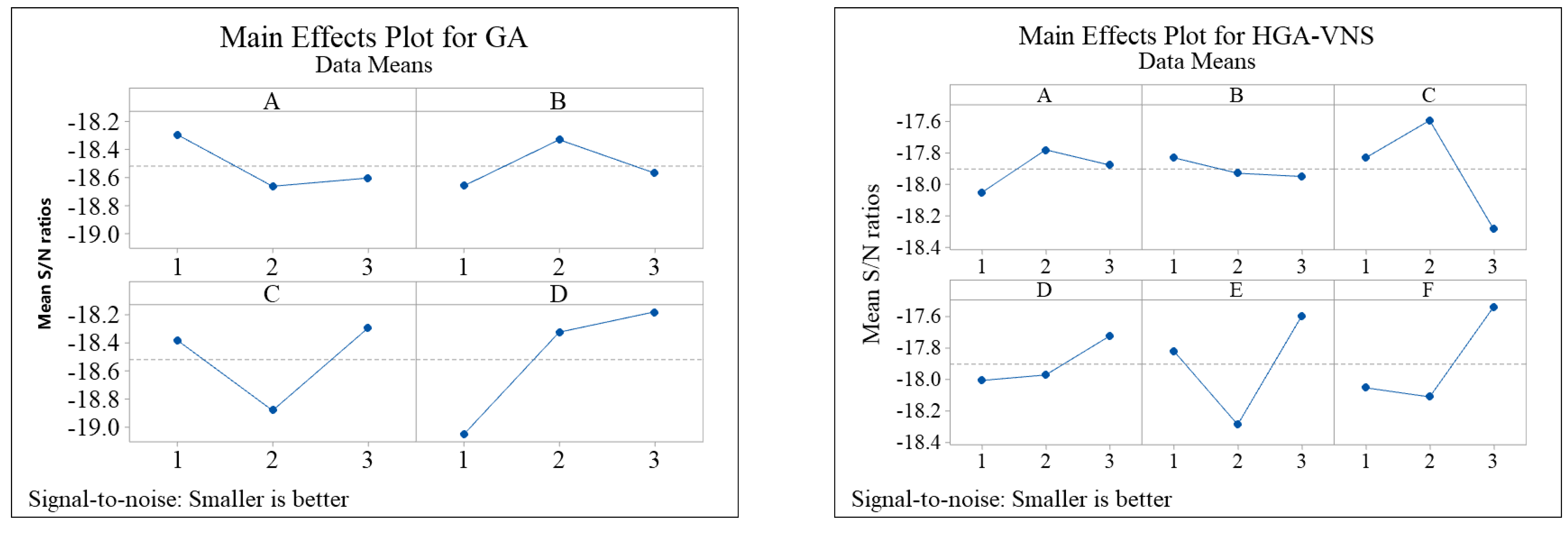
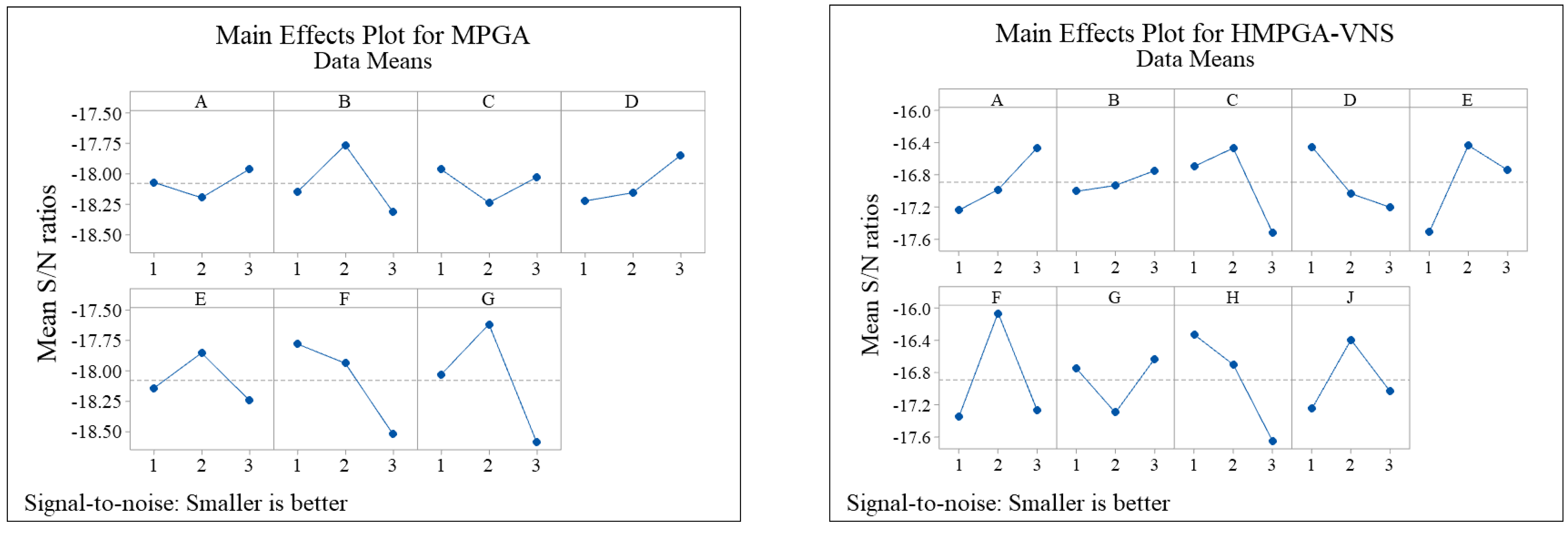
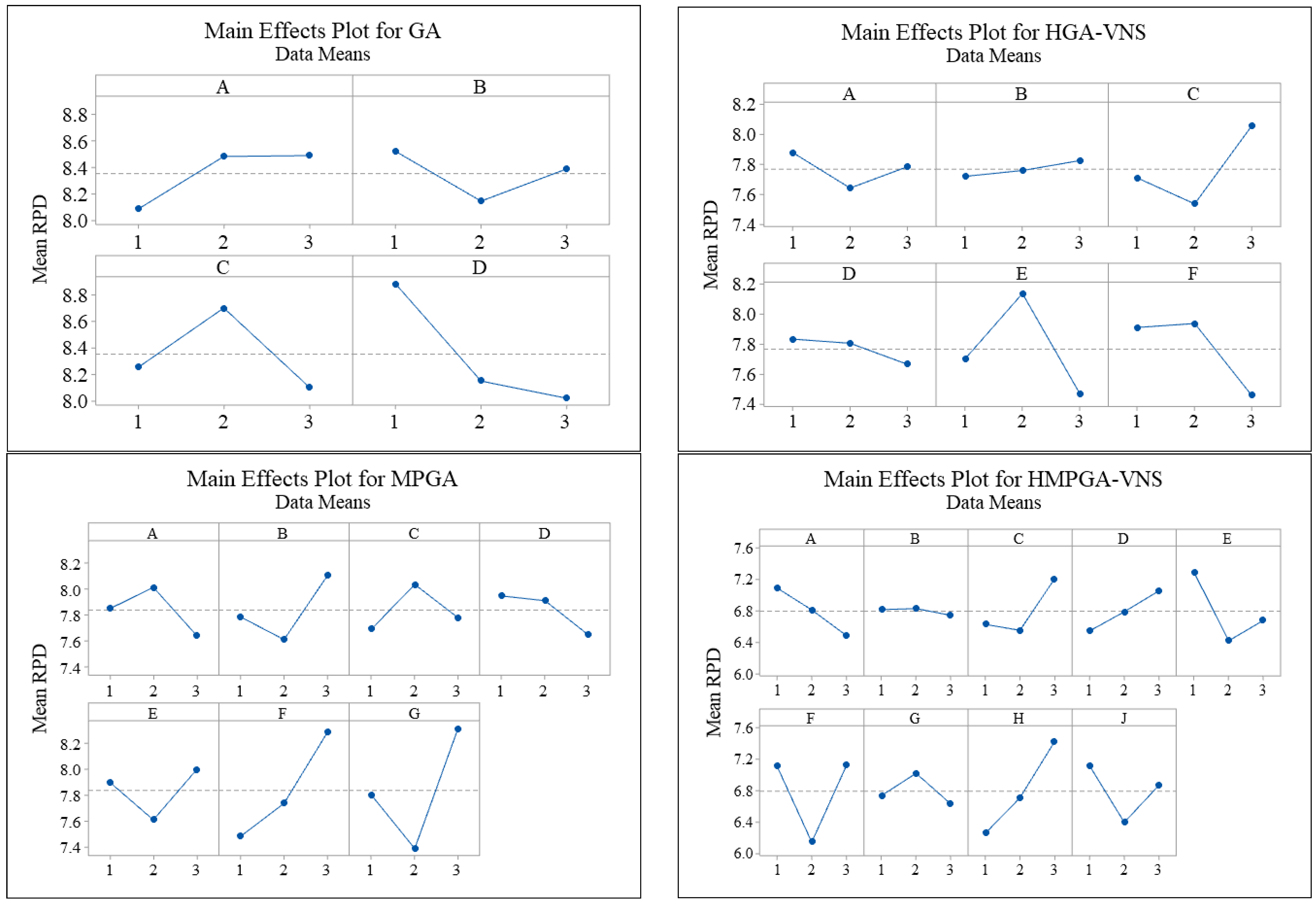
The S/N ratio output is analyzed by Minitab software to identify the optimal levels for each algorithm, as illustrated in Figure 4. The larger values of the S/N ratio indicate more robust algorithms, and these levels are considered as the optimal ones. For GA, the optimal levels are 1, 2, 3, and 3 for the respective parameters.
In addition to the S/N ratio, the RPD is employed as an additional measure for further analysis. Figure 5 presents the RPD results for each parameter level, indicating the best levels for the factors. These findings are consistent with the results obtained from the S/N ratio analysis.

4.3. Experimental Results

Based on the findings from the previous section, we adjust the parameters of the different metaheuristic algorithms. To ensure the reliability of the results, we conduct five replications for each experiment due to the random nature of the algorithms. The relative performance of the algorithms is evaluated by examining the effect of various problem sizes on their robustness. To assess the robustness of the algorithm, the impact of different problem sizes on their comparative performance is investigated.
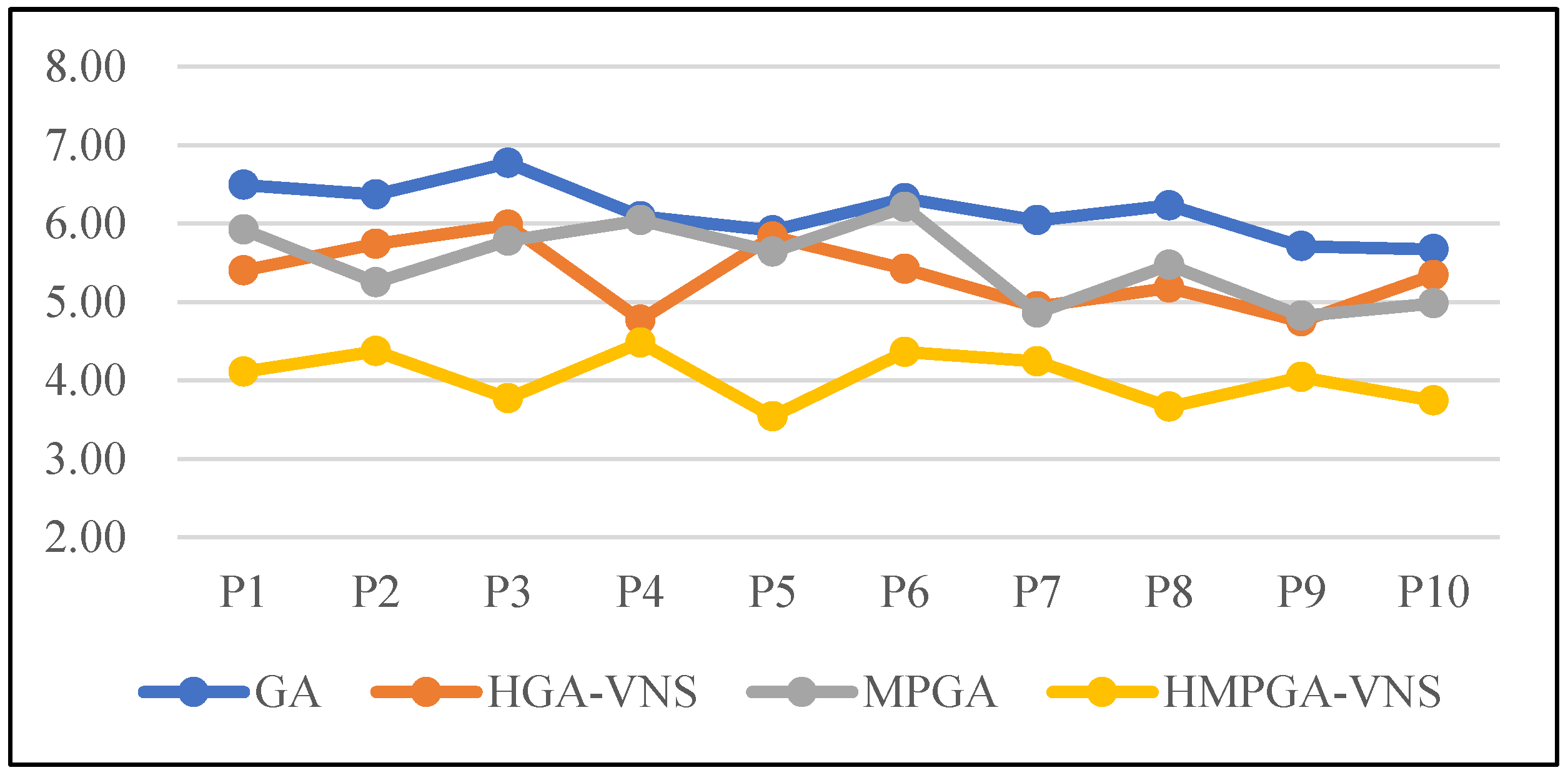
Figure 6 displays the inverse relationship between the algorithm’s capability and the size of the 10 problems considered. Each point presented in Figure 6 represents the means obtained using some algorithm from replicate experiments of the corresponding instances size described above. The best-performing algorithms are expected to exhibit consistently lower values with higher capacities. The graph highlights the outstanding performance of the HMPGA-VNS algorithm, which outperforms the other algorithms in the entire series.
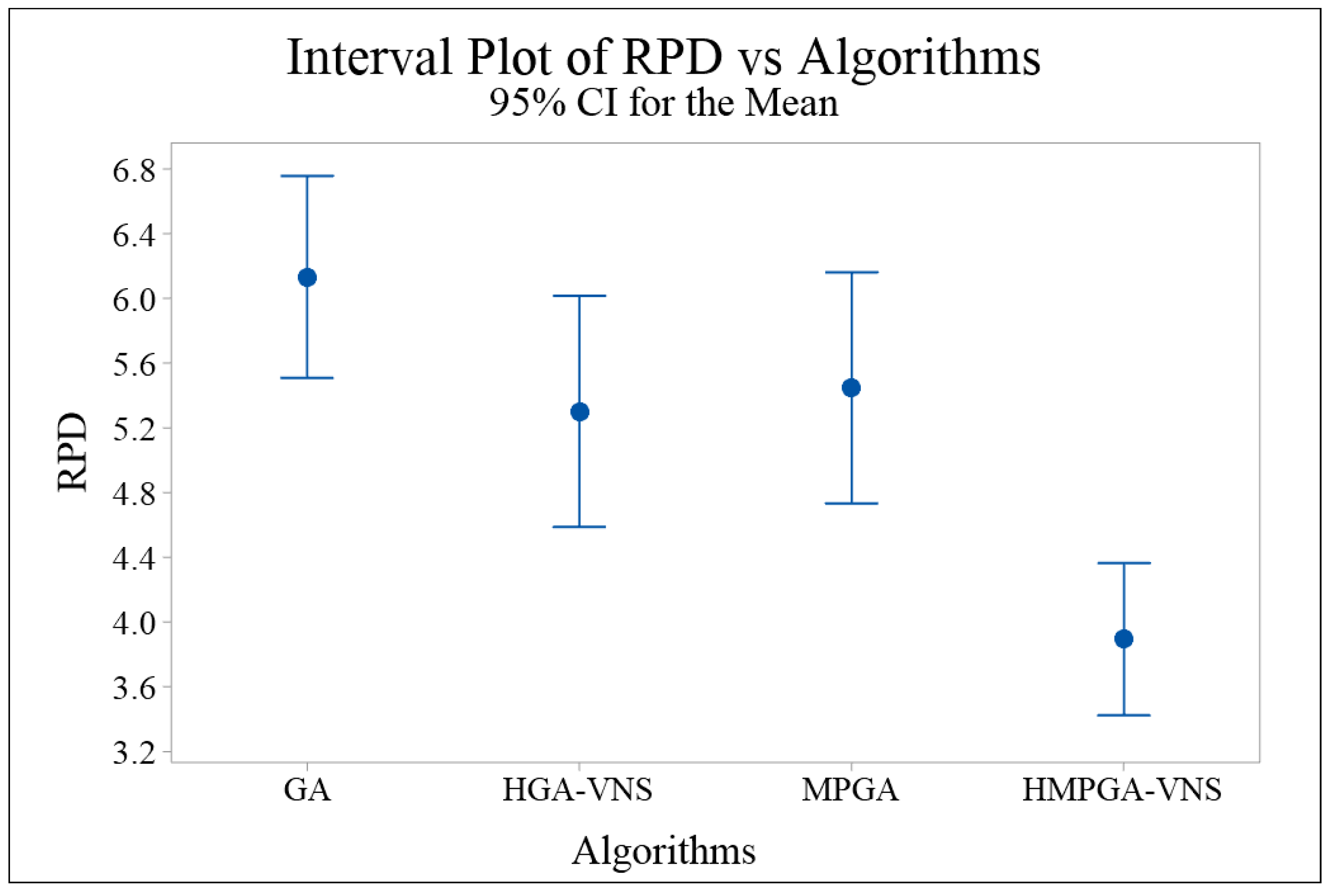
Furthermore, the performance of the various algorithms is further compared by analyzing the variance of the mean RPD of each algorithm for instances of different problem sizes. The analysis of variance (ANOVA) is utilized to obtain the means and least significant difference (LSD) intervals with a confidence level of 95% for each algorithm, as depicted in Figure 7. The statistical analysis indicates a significant difference in performance between HMPGA-VNS and all other algorithms. Remarkably, HMPGA-VNS outperforms all other algorithms, while the performance of the other algorithms, in terms of mean RPD, does not exhibit any significant difference.

4.4. Sensitivity Analysis

This section aims to examine how the solution is affected by demand, product shelf life, and waste rate. To achieve this, the different values for these parameters in P10 are analyzed.
Table 6 demonstrates that the objective function exhibits nearly linear behavior in response to changes in demand. Specifically, when the demand increases or decreases by 40%, the objective function correspondingly increases or decreases by 36.49%.
In Table 7, the results of the sensitivity analysis for product shelf life in two to six periods are presented. It is observed that extending the product shelf life leads to a reduction in the total cost of the supply chain.
Furthermore, Table 8 illustrates that reducing the waste rate can effectively minimize costs by decreasing transportation, production, and waste-related expenses.

4.5. Managerial Implications

The results of this study hold significant managerial implications, particularly for decision-makers and managers aiming to establish a supply chain for perishable products to meet the rapidly increasing market demand.
Firstly, the models and solutions developed in this study can be utilized to construct a PPSCN, effectively connecting manufacturers, DCs, and retailers. This approach enables a comprehensive reduction in supply chain costs from a global perspective. Additionally, the proposed model can be applied to optimize objectives in other food industries.
Furthermore, strategic planning of DCs, efficient inventory management, and effective route planning between DCs and retailers are vital in minimizing overall costs. During the planning process, decision-makers must carefully consider their specific circumstances, as any interconnection significantly impacts overall costs. The joint optimization of the PPSCN presents a significant challenge, and this study offers decision-makers a framework to consider all relevant factors when establishing a supply chain network for perishable products.
Lastly, the sensitivity analysis conducted in this study emphasizes the importance of focusing on product shelf life and waste rate to reduce supply chain costs. For instance, significant benefits can be achieved by improving product packaging. Therefore, managers in the perishable product industry should prioritize making sustainable decisions, which contribute to both economic growth and environmental sustainability.

5. Conclusions, Limitations, and Future Works

In this paper, a LIRP for the multi-echelon, multi-product, multi-period PPSCN was proposed. The characteristics of perishable products were considered in regard to the integrated decision problem. To solve the NP-hard problem, two hybrid metaheuristic algorithms, HGA-VNS and HMPGA-VNS, were proposed. A new chromosome representation was introduced to cater to the unique problem structure. Further, the Taguchi experimental design method was employed to tune the algorithm parameters. After solving the suggested model by the proposed algorithms, the results revealed that HMPGA-VNS outperforms HGA-VNS, MPGA, and GA. Lastly, a sensitivity analysis was conducted on the key parameters of the model to validate its effectiveness. Managerial implications are valuable for practitioners and managers who are involved in establishing a supply chain for perishable products.
This research, like other studies, has certain limitations that are described below:
  • In terms of the absence of an official dataset, randomly generated data were employed to conduct an experimental analysis. This approach may not fully represent real-world scenarios.
  • Like many other metaheuristic algorithms, the proposed algorithms in this study often lack theoretical guarantees or bounds on their performance. It can be challenging to evaluate the quality of solutions obtained or predict the behavior of the algorithms across different problem instances.
  • The effectiveness of the hybrid metaheuristic approaches presented in this paper relies on the coder’s proficiency in finding the initial solution.
For future research, the following points are recommended:
  • Enhancing the reliability and validity of the findings by incorporating realistic scenario datasets that are relevant to the PPSCN.
  • Exploring the exact methods such as the Lagrangian relaxation methods or Benders decomposition to achieve more precise results.
  • Investigating the application of new metaheuristic algorithms or developing novel heuristics to further optimize the results.

Author Contributions

Conceptualization, L.P.; Methodology L.P.; Software, L.P., and L.L.; Validation, M.S. and; Formal analysis, L.P. and; Investigation, L.P.; Resources L.L.; Data curation L.L.; Writing—original draft preparation, L.P.; Writing—review and editing, L.P. and M.S.; Visualization, L.P.; Supervision, L.L. and M.S.; Funding acquisition, L.L. All authors have read and agreed to the published version of the manuscript.

Funding

This research was funded by the National Natural Science Foundation of China, grant number 72004062.

Institutional Review Board Statement

Not applicable.

Informed Consent Statement

Not applicable.

Data Availability Statement

The datasets used and/or analyzed during the current study are available from the corresponding author upon reasonable request.

Acknowledgments

The authors would like to sincerely thank the editors, the anonymous reviewers, and the proofreaders for their constructive comments and suggestions.

Conflicts of Interest

The authors declare no conflict of interest.

References

  1. Ferguson, M.; Ketzenberg, M.E. Information sharing to improve retail product freshness of perishables. Prod. Oper. Manag. 2006, 15, 57–73. [Google Scholar] [CrossRef]
  2. Roberti, M.; Scheer, F.P. RFID will help keep perishables fresh. RFID J. 2005. Available online: http://www.rfidjournal.com/article/articleview/1775/1/1/ (accessed on 12 June 2023).
  3. Dai, Z.; Aqlan, F.; Zheng, X.T.; Gao, K. A location-inventory supply chain network model using two heuristic algorithms for perishable products with fuzzy constraints. Comput. Ind. Eng. 2018, 119, 338–352. [Google Scholar] [CrossRef]
  4. Jia, P.; Dong, Z. Analyses on the Way of Changing the Growth Mode of Circulation Economy. Asian Soc. Sci. 2009, 5, 53. [Google Scholar] [CrossRef] [Green Version]
  5. Liu, A.J.; Zhu, Q.Y.; Xu, L.; Lu, Q.; Fan, Y.Q. Sustainable supply chain management for perishable products in emerging markets: An integrated location-inventory-routing model. Transp. Res. Part E Logist. Transp. Rev. 2021, 150, 19. [Google Scholar] [CrossRef]
  6. Meidute-Kavaliauskiene, I.; Yildirim, F.; Ghorbani, S.; Cincikaite, R. The Design of a Multi-Period and Multi-Echelon Perishable Goods Supply Network under Uncertainty. Sustainability 2022, 14, 2472. [Google Scholar] [CrossRef]
  7. Akram, H.W.; Akhtar, S.; Ahmad, A.; Anwar, I.; Sulaiman, M. Developing a Conceptual Framework Model for Effective Perishable Food Cold-Supply-Chain Management Based on Structured Literature Review. Sustainability 2023, 15, 4907. [Google Scholar] [CrossRef]
  8. Liu, L.H.; Lee, L.S.; Seow, H.V.; Chen, C.Y. Logistics Center Location-Inventory-Routing Problem Optimization: A Systematic Review Using PRISMA Method. Sustainability 2022, 14, 15853. [Google Scholar] [CrossRef]
  9. Ali, S.; Bhargava, A.; Saxena, A.; Kumar, P. A Hybrid Marine Predator Sine Cosine Algorithm for Parameter Selection of Hybrid Active Power Filter. Mathematics 2023, 11, 598. [Google Scholar] [CrossRef]
  10. Govindan, K.; Jafarian, A.; Nourbakhsh, V. Designing a sustainable supply chain network integrated with vehicle routing: A comparison of hybrid swarm intelligence metaheuristics. Comput. Oper. Res. 2019, 110, 220–235. [Google Scholar] [CrossRef]
  11. Goodarzian, F.; Taleizadeh, A.A.; Ghasemi, P.; Abraham, A. An integrated sustainable medical supply chain network during COVID-19. Eng. Appl. Artif. Intell. 2021, 100, 104188. [Google Scholar] [CrossRef]
  12. Wu, T.; Shen, H.C.; Zhu, C. A multi-period location model with transportation economies-of-scale and perishable inventory. Int. J. Prod. Econ. 2015, 169, 343–349. [Google Scholar] [CrossRef]
  13. Gholami-Zanjani, S.M.; Jabalameli, M.S.; Klibi, W.; Pishvaee, M.S. A robust location-inventory model for food supply chains operating under disruptions with ripple effects. Int. J. Prod. Res. 2021, 59, 301–324. [Google Scholar] [CrossRef]
  14. Savadkoohi, E.; Mousazadeh, M.; Torabi, S.A. A possibilistic location-inventory model for multi-period perishable pharmaceutical supply chain network design. Chem. Eng. Res. Des. 2018, 138, 490–505. [Google Scholar] [CrossRef]
  15. Hamdan, B.; Diabat, A. A two-stage multi-echelon stochastic blood supply chain problem. Comput. Oper. Res. 2019, 101, 130–143. [Google Scholar] [CrossRef]
  16. Liu, M.; Tang, H.; Wang, Y.F.; Li, R.X.; Liu, Y.; Liu, X.; Wang, Y.Q.; Wu, Y.Y.; Wu, Y.; Sun, Z.J. Enhancing Food Supply Chain in Green Logistics with Multi-Level Processing Strategy under Disruptions. Sustainability 2023, 15, 917. [Google Scholar] [CrossRef]
  17. Coelho, L.C.; Laporte, G. Optimal joint replenishment, delivery and inventory management policies for perishable products. Comput. Oper. Res. 2014, 47, 42–52. [Google Scholar] [CrossRef]
  18. Diabat, A.; Abdallah, T.; Le, T. A hybrid tabu search based heuristic for the periodic distribution inventory problem with perishable goods. Ann. Oper. Res. 2016, 242, 373–398. [Google Scholar] [CrossRef]
  19. Le, T.; Diabat, A.; Richard, J.P.; Yih, Y. A column generation-based heuristic algorithm for an inventory routing problem with perishable goods. Optim. Lett. 2013, 7, 1481–1502. [Google Scholar] [CrossRef]
  20. Dai, Z.; Gao, K.; Giri, B.C. A hybrid heuristic algorithm for cyclic inventory-routing problem with perishable products in VMI supply chain. Expert Syst. Appl. 2020, 153, 113322. [Google Scholar] [CrossRef]
  21. Azadeh, A.; Elahi, S.; Farahani, M.H.; Nasirian, B. A genetic algorithm-Taguchi based approach to inventory routing problem of a single perishable product with transshipment. Comput. Ind. Eng. 2017, 104, 124–133. [Google Scholar] [CrossRef]
  22. Rohmer, S.U.K.; Claassen, G.D.H.; Laporte, G. A two-echelon inventory routing problem for perishable products. Comput. Oper. Res. 2019, 107, 156–172. [Google Scholar] [CrossRef]
  23. Wu, X.; Nie, L.; Xu, M. Designing an integrated distribution system for catering services for high-speed railways: A three-echelon location routing model with tight time windows and time deadlines. Transp. Res. Part C Emerg. Technol. 2017, 74, 212–244. [Google Scholar] [CrossRef]
  24. Zhu, S.X.; Ursavas, E. Design and analysis of a satellite network with direct delivery in the pharmaceutical industry. Transp. Res. Part E Logist. Transp. Rev. 2018, 116, 190–207. [Google Scholar] [CrossRef]
  25. Chen, C.; Tian, Z.; Yao, B. Optimization of two-stage location–routing–inventory problem with time-windows in food distribution network. Ann. Oper. Res. 2019, 273, 111–134. [Google Scholar] [CrossRef]
  26. Zandkarimkhani, S.; Mina, H.; Biuki, M.; Govindan, K. A chance constrained fuzzy goal programming approach for perishable pharmaceutical supply chain network design. Ann. Oper. Res. 2020, 295, 425–452. [Google Scholar] [CrossRef]
  27. Rafie-Majd, Z.; Pasandideh, S.H.R.; Naderi, B. Modelling and solving the integrated inventory-location-routing problem in a multi-period and multi-perishable product supply chain with uncertainty: Lagrangian relaxation algorithm. Comput. Chem. Eng. 2018, 109, 9–22. [Google Scholar] [CrossRef]
  28. Hiassat, A.; Diabat, A.; Rahwan, I. A genetic algorithm approach for location-inventory-routing problem with perishable products. J. Manuf. Syst. 2017, 42, 93–103. [Google Scholar] [CrossRef]
  29. Partovi, F.; Seifbarghy, M.; Esmaeili, M. Revised solution technique for a bi-level location-inventory-routing problem under uncertainty of demand and perishability of products. Appl. Soft. Comput. 2023, 133, 109899. [Google Scholar] [CrossRef]
  30. Aghighi, A.; Goli, A.; Malmir, B.; Tirkolaee, E.B. The stochastic location-routing-inventory problem of perishable products with reneging and balking. J. Ambient. Intell. Humaniz. Comput. 2021, 14, 6497–6516. [Google Scholar] [CrossRef]
  31. Biuki, M.; Kazemi, A.; Alinezhad, A. An integrated location-routing-inventory model for sustainable design of a perishable products supply chain network. J. Clean. Prod. 2020, 260, 120842. [Google Scholar] [CrossRef]
  32. Mladenovi, N.; Hansen, P.J.C.; Research, O. Variable Neighborhood Search. Comput. Oper. Res 1997, 24, 1097–1100. [Google Scholar] [CrossRef]
  33. Rath, S.; Gutjahr, W.J. A math-heuristic for the warehouse location-routing problem in disaster relief. Comput. Oper. Res. 2014, 42, 25–39. [Google Scholar] [CrossRef]
  34. Almouhanna, A.; Quintero-Araujo, C.L.; Panadero, J.; Juan, A.A.; Khosravi, B.; Ouelhadj, D. The location routing problem using electric vehicles with constrained distance. Comput. Oper. Res. 2020, 115, 104864. [Google Scholar] [CrossRef]
  35. Zhao, C.X.; Chen, J.H.; Zhang, X.C.; Cui, Z.Y. Solution of Multi-Crew Depots Railway Crew Scheduling Problems: The Chinese High-Speed Railway Case. Sustainability 2022, 14, 491. [Google Scholar] [CrossRef]
  36. Zegordi, S.H.; Nia, M.A.B. A multi-population genetic algorithm for transportation scheduling. Transp. Res. Part E Logist. Transp. Rev. 2009, 45, 946–959. [Google Scholar] [CrossRef]
  37. Cochran, J.K.; Horng, S.M.; Fowler, J.W. A multi-population genetic algorithm to solve multi-objective scheduling problems for parallel machines. Comput. Oper. Res. 2003, 30, 1087–1102. [Google Scholar] [CrossRef]
  38. Pourvaziri, H.; Naderi, B. A hybrid multi-population genetic algorithm for the dynamic facility layout problem. Appl. Soft. Comput. 2014, 24, 457–469. [Google Scholar] [CrossRef]
  39. Wang, T.; Wang, Q.Y.; Zhang, C.Q. Research on the Optimal Operation of a Novel Renewable Multi-Energy Complementary System in Rural Areas. Sustainability 2021, 13, 2196. [Google Scholar] [CrossRef]
  40. Hajiaghaei-Keshteli, M.; Molla-Alizadeh-Zavardehi, S.; Tavakkoli-Moghaddam, R. Addressing a nonlinear fixed-charge transportation problem using a spanning tree-based genetic algorithm. Comput. Ind. Eng. 2010, 59, 259–271. [Google Scholar] [CrossRef]
  41. Tavana, M.; Santos-Arteaga, F.J.; Mahmoodirad, A.; Niroomand, S.; Sanei, M. Multi-stage supply chain network solution methods: Hybrid metaheuristics and performance measurement. Int. J. Syst. Sci. Oper. Logist. 2018, 5, 356–373. [Google Scholar] [CrossRef]
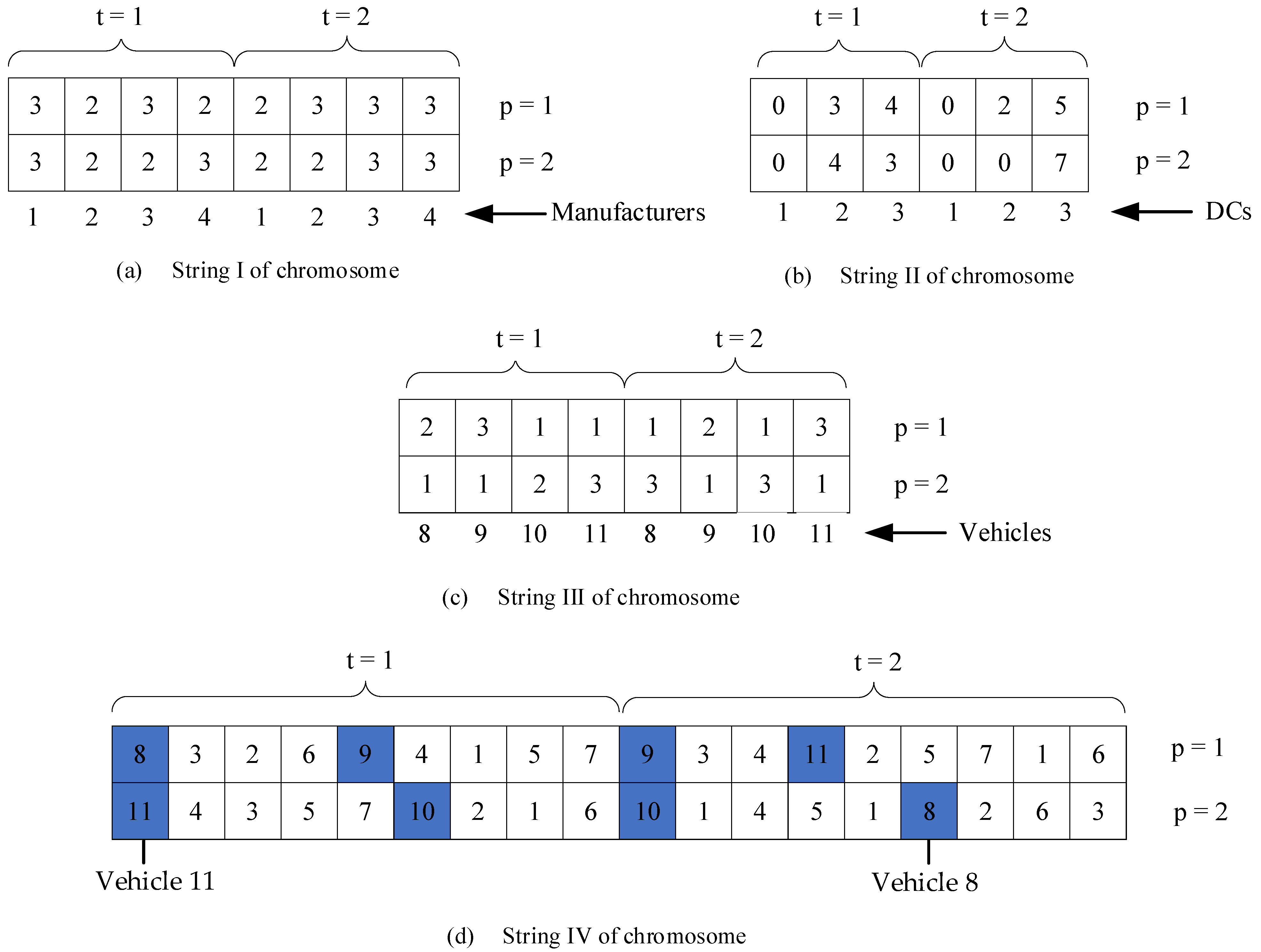
Figure 1. Chromosome representation.
Sustainability 15 10711 g001
Figure 2. Crossover operator.
Sustainability 15 10711 g002
Figure 3. Mutation operator.
Sustainability 15 10711 g003
Figure 4. Mean S/N ratios plot for each level of the factors (factors represented by capitalized letter in each subfigure are consistent with Table 4).
Sustainability 15 10711 g004aSustainability 15 10711 g004b
Figure 5. Mean RPD plot for each level of the factors (factors represented by capitalized letter in each subfigure are consistent with Table 4).
Sustainability 15 10711 g005
Figure 6. Means plot for the interaction between each algorithm and instances.
Sustainability 15 10711 g006
Figure 7. Means plot and LSD intervals for the Algorithms.
Sustainability 15 10711 g007
Table 1. Comparison of our work and related literature.
ReferenceProblemAssumptionsSolution Methods
LIRPMulti-ProductMulti-PeriodDamage in
Inventory Process
Damage in
Transportation Process
Specific Shelf Life
Chen et al. (2019) [25]----Hybrid heuristic
Zandkarimkhani et al. (2020) [26]---Hybrid approach
Rafie-Majd et al. (2018) [27]-Lagrangian relaxation algorithm
Hiassat et al. (2017) [28]----GA
Partovi et al. (2023) [29]----Revised solution technique
Aghighi et al. (2021) [30]-----Improved GA
Biuki et al. (2020) [31]--Hybrid GA-PSO
Liu et al. (2021) [5]---YALMIP toolbox
This studyHybrid GA-VNS, hybrid MPGA-VNS
Table 2. Uniform distributions of random parameters.
ParameterRangeParameterRangeParameterRange
f i 1 105 U (3.0, 4.0) f j 2 105 U (1.5, 2.0) r c p U (30, 50)
p c i p U (80, 100) t c l n v p 2 U (0.4, 0.5) d k p t U (30, 60)
t c i j p 1 U (0.2, 0.3) h c j p U (30, 40) v v p c a p U (200, 300)
m j p t c a p U (1000, 1500) A % U (10, 30) τ p U (3, 5)
Table 3. Instance size.
Instance No.|I| – |J| – |K| – |P| – |V| – |T|Instance No.|I| – |J| – |K| – |P| – |V| – |T|
P12 – 2 – 5 – 2 – 2 – 2P63 – 4 – 18 – 4 – 4 – 4
P22 – 2 – 8 – 2 – 2 – 2P73 – 5 – 20 – 5 – 5 – 5
P32 – 3 – 10 – 3 – 3 – 3P83 – 5 – 25 – 5 – 5 – 5
P42 – 3 – 12 – 3 – 3 – 3P93 – 6 – 30 – 6 – 6 – 6
P52 – 4 – 15 – 4 – 4 – 4P103 – 6 – 37 – 6 – 6 – 6
Table 4. Factors and their levels.
GA FactorsGA LevelsHGA-VNS FactorsHGA-VNS Levels
P A1: 120 A2: 240 A3: 360 P A1: 120 A2: 240 A3: 360
M a x _ i t e r B1: 400 B2: 600 B3: 800 M a x _ i t e r B1: 400 B2: 600 B3: 800
P c C1: 0.70 C2: 0.75 C3: 0.80 P c C1: 0.70 C2: 0.75 C3: 0.80
P m D1: 0.10 D2: 0.15 D3: 0.20 P m D1: 0.10 D2: 0.15 D3: 0.20
MaxiterE1: 100 E2: 200 E3: 300
N l F1: 3 F2: 4 F3: 5
MPGA FactorsMPGA LevelsHMPGA-VNS FactorsHMPGA-VNS Levels
P A1: 120 A2: 240 A3: 360 P A1: 120 A2: 240 A3: 360
M a x _ i t e r B1: 400 B2: 600 B3: 800 M a x _ i t e r B1: 400 B2: 600 B3: 800
P c C1: 0.70 C2: 0.75 C3: 0.80 P c C1: 0.70 C2: 0.75 C3: 0.80
P m D1: 0.10 D2: 0.15 D3: 0.20 P m D1: 0.10 D2: 0.15 D3: 0.20
S P E1: 20 E2: 30 E3: 40 S P E1: 20 E2: 30 E3: 40
M p F1: 10 F2: 20 F3: 40 M p F1: 10 F2: 20 F3: 40
M s G1: 4 G2: 6 G3: 8 M s G1: 4 G2: 6 G3: 8
MaxiterH1: 100 H2: 200 H: 300
N l I1: 3 I2: 4 I3: 5
Table 5. The orthogonal array L9 for GA.
L9ABCD
11111
21222
31333
42123
52231
62312
73132
83213
93321
Table 6. Sensitivity analysis in demand.
Change of Demand−40%−20%Base Case20%40%
Objective value12,354,318.1915,789,639.5419,452,555.8023,154,377.1727,177,165.7
Sensitivity (%)−36.49−18.83019.0339.71
Table 7. Sensitivity analysis in product shelf life.
Product Shelf Life23Base Case56
Objective value19,966,103.2719,645,136.1019,452,555.8019,263,866.0019,176,329.51
Sensitivity (%)2.640.990−0.97−1.42
Table 8. Sensitivity analysis in product transportation loss rate.
Change of Waste Rate−40%−20%Base Case20%40%
Objective value18,318,471.7918,865,088.6119,452,555.8020,242,329.5721,255,807.72
Disclaimer/Publisher’s Note: The statements, opinions and data contained in all publications are solely those of the individual author(s) and contributor(s) and not of MDPI and/or the editor(s). MDPI and/or the editor(s) disclaim responsibility for any injury to people or property resulting from any ideas, methods, instructions or products referred to in the content.