Day-Ahead and Intra-Day Optimal Scheduling Considering Wind Power Forecasting Errors

Abstract

The aim of this paper is to address the challenges regarding the safety and economics of power system operation after the integration of a high proportion of wind power. In response to the limitations of the literature, which often fails to simultaneously consider both aspects, we propose a solution based on a stochastic optimization scheduling model. Firstly, we consider the uncertainty of day-ahead wind power forecasting errors and establish a multi-scenario day-ahead stochastic optimization scheduling model. By balancing the reserve capacity and economic efficiency in the optimization scheduling, we obtain optimized unit combinations that are applicable to various scenarios. Secondly, we account for the auxiliary service constraints of thermal power units participating in deep peak shaving, and develop an intra-day dynamic economic dispatch model. Through the inclusion of thermal power units and energy storage units in the optimization scheduling, the accommodation capacity of wind power is further enhanced. Lastly, in the electricity market environment, increasing wind power capacity can increase the profits of thermal power peak shaving. However, we observe a trend of initially increasing and subsequently decreasing wind power profits as the wind power capacity increases. Considering system flexibility and the curtailed wind power rate, it is advisable to moderately install grid-connected wind power capacity within the power system. In conclusion, our study demonstrates the effectiveness of the proposed scheduling model in managing day-ahead uncertainty and enhancing the accommodation of wind power.

1. Introduction

With the increasing integration of a high proportion of wind power into the grid, the uncertainty of wind power forecasting errors has a significant impact on the safety and economics of system operation. In this study, we consider the uncertainty of day-ahead wind power forecasting errors and propose a day-ahead stochastic optimization scheduling model. This model effectively resolves the trade-off between reserving spare capacity and sacrificing economic efficiency, while ensuring reliable system operation. In addition, we develop an intra-day dynamic economic dispatch considering the ancillary service constraints for thermal units participating in deep peak shaving. By employing both deep peak shaving of thermal units and optimized scheduling with energy storage systems, we further enhance the integration capability of wind power and address the economic challenges during system operation.

To achieve the “dual carbon” target, the weight index of non-hydraulic renewable energy consumption responsibility of each province (region or municipality directly under the Central Government) in China is gradually increasing year by year [1]. It is necessary to continuously increase the proportion of new energy installed capacity and green power trading to meet the weight index. With the high proportion of wind power integration, the problem of wind power curtailment has been further exacerbated, and higher requirements have been put forward for grid peak regulation capacity [2,3]. In the electricity market environment, the main source of electricity, namely thermal power, has gradually transformed from a provider of electricity to auxiliary services. Therefore, it is necessary to fully utilize the deep peak regulation capacity of thermal power units in both the intra-day and day-ahead stages. On the one hand, it increases the revenue of thermal power, and on the other hand, it effectively reduces the curtailed electricity of wind power and improves its utilization rate, achieving an ideal situation.

Regarding the randomness of large-scale wind power, the main methods adopted domestically and internationally are as follows: (1) modeling method with sufficient rotating reserve capacity reserved, which sacrifices the economic efficiency of system operation to some extent [4]; (2) stochastic modeling method based on chance constraints [5,6], where corresponding constraint conditions are described in the form of probability, but it is difficult to deduce the chance constraint model for large-scale power systems; (3) stochastic optimization method based on scenario generation [7,8], which is applied to stochastic optimization scheduling considering wind power prediction error and can take into account the safety and economic efficiency of system operation, without considering reserved rotating reserve capacity, and the stochastic optimization unit combination obtained has universality for possible scenarios.

To promote the construction of a new type of power system, China National Energy Administration has issued the “Management Measures for Power Auxiliary Services”, which put higher requirements on the demand for auxiliary service resources such as power system peak regulation, standby, and ramp-up in the electricity market environment [9]. Traditional intra-day dynamic economic dispatch models [10,11] have not considered the auxiliary service constraints in market transactions. Reference [12] considered the constraint of proactive regulation of thermal power units and established a multi-energy complementary coordinated optimization dispatch. To address the problem of constraint conditions and variables, a hierarchical optimization dispatch was adopted, which provided helpful insights for this paper but did not consider the stochasticity of wind power forecast errors. In [13], while in the intra-day time scale, the predicted values of wind power, solar power, and load power are represented by fuzzy parameters and used to adjust the output of units. However, the article overlooked the day-ahead forecasts for wind and solar power, which led to inaccurate representation of uncertainties and limited its application.

Different algorithms such as fuzzy logic [14,15], TLBO [16,17], ANN [18], and other intelligent artificial algorithms have both advantages and disadvantages compared to the random optimization algorithm discussed in this article. Fuzzy logic is capable of handling problems with uncertain or incomplete data and making decisions based on fuzzy rules [19]. However, it may lack the ability to handle complex optimization problems with a large number of variables or constraints, making it more suitable for optimization scheduling with longer time periods such as monthly or quarterly cycles. TLBO is an optimization algorithm based on swarm intelligence, simulating the teaching and learning process in a classroom [20]. However, it may suffer from slow convergence and being prone to entrapment in local optima when dealing with complex problems. The optimization results may also be affected by the initial solution selection and learning rate parameters. An ANN is an artificial intelligence algorithm that mimics the structure and functionality of biological neural networks [21]. It is powerful in handling pattern recognition and nonlinear problems but may require a large amount of training data and computational resources. The newer artificial intelligence algorithms such as fuzzy logic, TLBO, and ANN generally require more computational resources and higher implementation complexity. Additionally, selecting the appropriate sample size for intelligent algorithm implementation can be challenging, as both too-large and too-small sample sizes may yield estimated solutions rather than accurate values. The simulation time for these algorithms can also be quite long. On the other hand, the two-stage optimization approach has the advantage of explicitly separating the day-ahead and intra-day stages, allowing for more accurate modeling of uncertainties and more detailed economic dispatch decisions. The solutions obtained from this approach are accurate values rather than estimates, taking into account the specific characteristics of the power system. Overall, each algorithm has its own strengths and limitations. When choosing a suitable algorithm, it is important to consider the characteristics of the problem, computational resources available, and the desired precision of the solutions.

The literature has primarily focused on either the safety or economics of system operation after the integration of a high proportion of wind power, without considering both aspects simultaneously. In light of this gap, our paper addresses this issue by considering the day-ahead optimization scheduling stage. We incorporate the day-ahead wind power forecasting results and the probability distribution of historical forecasting errors to establish a stochastic optimization scheduling model. This approach ensures the reliability of system operation and avoids subjective factors based on ambiguity. Furthermore, we resolve the trade-off between reserving spare capacity and sacrificing economic efficiency. In the intra-day optimization scheduling stage, traditional dynamic economic dispatch models do not account for the auxiliary service constraints imposed by market transactions. As a result, the benefits accrued by wind power and thermal power units participating in the electricity market are limited. To overcome this limitation, our paper considers the auxiliary service constraints for thermal power units involved in deep peak shaving and establishes an intra-day dynamic economic dispatch model. This further enhances the integration capacity of renewable energy sources by allowing for improved consumption.

This paper is structured as follows: Section 2 introduces a stochastic wind power output scenario. Section 3 establishes a stochastic optimization scheduling model considering forecasting errors for day-ahead operations. Section 4 presents a dynamic economic scheduling model for intra-day operations considering deep peak shaving of thermal generation. Finally, Section 5 discusses the simulation results, followed by the conclusions in Section 6.

2. Stochastic Wind Power Output Scenario

Wind power prediction is subject to errors caused by the uncertainty of wind power and the influence of prediction methods and data sources. The presence of errors in forecast results is inevitable. With current forecasting technologies, short-term errors typically range from 10% to 30% [22,23], while day-ahead forecasting errors are generally around 10% [23,24,25]. To deal with the uncertainty in wind power forecasting, the focus is mainly on dealing with the randomness of forecast errors.

2.1. Method of Handling Randomness

The method of stochastic processing involves analyzing historical wind power generation data, building statistical models, and using these models to estimate prediction errors. Common methods for wind power forecasting are based on modeling forecast errors using known distributions such as the Gaussian [26,27], Beta [28,29], Laplace [30], Weibull [31], Cauchy [32], and Gamma [27]. These methods statistically analyze forecast errors and accurately fit the variations in wind power within different forecast ranges. Based on the stochastic modeling concept of uncertainty, incorporating the probability distribution information of historical forecast errors and current wind power forecast results eliminates subjective factors based on fuzziness, especially when the distribution models are deterministic. In such cases, the probability density function (PDF), cumulative distribution function (CDF), and inverse function are all explicitly expressed, which greatly facilitates solving the problems in practical applications and meets the requirements for accurate fitting.

Based on the time series of wind forecasts, the sub-interval to which the predicted value belongs at a certain moment is determined. In engineering applications, the t location–scale distribution model is usually used to establish the probability distribution of actual power values within the sub-interval, which has better fitting effect than normal distribution [33]. Meanwhile, considering the correlation between the wind power output at different time sections, this paper uses the multivariate normal distribution function to describe the correlation in time. The dynamic scenarios are generated through the inverse transformation sampling method. To improve the calculation efficiency, the scenario reduction is carried out, retaining the scenario set with the highest probability of occurrence.

2.2. Establishment of Prediction Box

Based on historical data, a “prediction box” for [actual power values, predicted values] is established, and the predicted values are normalized and divided into M equal sub-intervals ranging from 0 to 1. Each sub-interval is [0, 1/M], [1/M, 2/M], …, [(M − m)/M, m/M], …, [(M − 1)/M, 1], and a probability distribution based on prediction errors is established.

2.3. T Location–Scale Distribution

The power distribution of actual power in sub-intervals is represented using t location–scale, and its probability density function (PDF) is

$$\mathrm{f}(x)=\frac{\Gamma (\frac{\upsilon +1}{2})}{\sigma \sqrt{\upsilon \pi } \Gamma (\frac{\upsilon }{2})}{\left(1+\frac{{\left(\frac{x-\mu }{\sigma }\right)}^2}{\upsilon }\right)}^{-\frac{\upsilon +1}{2}}$$

(1)

where $\Gamma \left(x\right)$ is the Gamma function, $\upsilon >0$ is the shape parameter, $\sigma >0$ is the scale parameter, and $\mu$ is the location parameter.

The location parameter of the t location–scale distribution does not change the shape of the curve; it just shifts it horizontally along the axis. If the parameter is positive, the curve is shifted to the right. On the other hand, the scale parameter determines the concentration level of the power prediction errors and shapes the graph of the t location–scale distribution function. A smaller scale parameter value will result in a “tall and narrow” curve, indicating a more concentrated distribution and smaller power prediction errors. Conversely, a larger scale parameter value will result in a “short and wide” curve, indicating a more dispersed distribution and larger power prediction errors. Therefore, the size of the scale parameter can affect the shape of the t location–scale distribution. In practical applications, it is necessary to select an appropriate scale parameter value based on specific circumstances to accurately describe the data distribution.

2.4. Dynamic Scenario Generation

The time series $\mathrm{P}={({\mathrm{P}}_1,{\mathrm{P}}_2,\dots ,{\mathrm{P}}_t)}^T$ of wind power can be viewed as a multivariate random vector, with $t$ as the forecast length. To characterize the correlation between each time section, assume that $P$ follows a multivariate normal distribution $P\sim N({\mu }_0,\mathsf{\Sigma })$, with expectation ${\mu }_0$ as a zero vector of $t$ dimensions, and covariance matrix B as follows:

$$\Sigma =\left[\begin{array}{cccc}{\sigma }_{1,1}& {\sigma }_{1,2}& \cdots & {\sigma }_{1,t}\\ {\sigma }_{2,1}& {\sigma }_{2,2}& \cdots & {\sigma }_{2,t}\\ ⋮& ⋮& \ddots & ⋮\\ {\sigma }_{t,1}& {\sigma }_{t,2}& \cdots & {\sigma }_{t,t}\end{array}\right]$$

(2)

where ${\sigma }_{i,j}=\mathrm{cov}(P_i,P_j)$ is the covariance between random variables $P_i$ and $P_j$, $i,j=1,2,\cdots ,t$. Modeling is performed using an exponential type of covariance:

$${\sigma }_{i,j}=\mathrm{cov}(P_i,P_j)=\exp \left(-\frac{\left|i-j\right|}{\epsilon }\right),0\le i,j\le t$$

(3)

The parameter $\epsilon$ represents the strength of correlation. To obtain the optimal parameter $\epsilon$ values, we establish the objective function:

$$\min I_{\epsilon }=\frac{1}{N}{\displaystyle \sum _{s\in S}\left|pdf(s)-pd{f}^{\prime }(s)\right|}$$

(4)

where $S$ is the set of equidistant sampling points, $N$ is the sampling size, and $pdf(s)$ and $pd{f}^{\prime }(s)$ are the probability density function values of the t location–scale fit of dynamic scenarios and wind power historical data, respectively.

In order to avoid the problem of low sampling efficiency due to small sample size and repeated sampling, the Latin hypercube sampling (LHS) technique [34,35]. is used to ensure that sampling points cover the sampling set area uniformly. The random numbers obtained from sampling are transformed by inverse transformation on t location–scale to obtain the optimal dynamic scenario set.

2.5. Scenario Reduction

The generation of a large number of dynamic scenarios increases the complexity of computation. To reduce this, synchronous backward elimination method is employed for scenario reduction [36], which obtains a small number of scenarios with higher probabilities. The specific steps are as follows:

• Set the initial probability of each generated scenario to $p_s=1/N,(s=1,2,\cdots ,N)$, calculate the probability distance $D{T}_{s,s^{\prime }}$ between two scenarios, which is the vector norm of scenario $s$ and scenario $s^{\prime }$. The scenarios to be eliminated are represented as $DS$, which is initialized as an empty set.
• For each scenario $k$, there is a scenario $r$ with the minimum probability distance to all other scenarios, denoted as $D{T}_k(r)=\min D{T}_{k,s^{\prime }},k\in S,s^{\prime }\in S,k\ne s^{\prime }$, $S$ being the original set of scenarios.
• Calculate $P{D}_k(r)=p_k\ast D{T}_k(r),k\in S,$ such that $P{D}_d=\min P{D}_k,k\in S$, repeat step (2) until the number of remaining scenarios reaches the specified threshold.

3. Considering Random Optimization Scheduling of Day-Ahead Forecast Errors

Establish a two-stage optimization scheduling model, where the first stage optimizes the economic efficiency of thermal power and minimizes wind power curtailment, taking into account the uncertainty of wind power day-ahead forecasting errors, conventional constraints of power plants, grid constraints, power balance, etc. Through stochastic optimization scheduling, the optimal combination of power generation units is obtained. In the second stage, with the power generation unit combination determined in the first stage, the objective is to maximize the peak regulation benefit of thermal power units and wind power profit, considering the constraints of thermal power units participating in deep peak regulation. Through dynamic economic dispatch, the space for new energy consumption is further improved.

3.1. Objective Function

3.1.1. Thermal Power Unit Conventional Operating Cost Model

Wind power operating costs are ignored, and the system cost mainly depends on the fuel cost and start-up cost of thermal power units. The objective function is as follows:

$$\mathrm{F}=\min {\displaystyle \sum _{s=0}^{N_s}{\displaystyle \sum _{i=1}^{N_g}{\displaystyle \sum _{t=1}^{N_T} p_s}\times }}{f}_1(P_{s,i,t})+{\displaystyle \sum _{i=1}^{N_g}{\displaystyle \sum _{t=1}^{N_T} f_2(u_{i,t})}}$$

(5)

$$f_1(P_{s,i,t})=a_i{P}_{s,i,t}^2+b_i{P}_{s,i,t}+c_i$$

(6)

$$f_2(u_{i,t})=u_{i,t}\times (1-u_{i,t-1})\times D_i$$

(7)

where $F$ is the system cost, where $f_1(P_{s,i,t})$ represents the fuel cost of unit $i$ in scenario $s$ at time $t$, $u_{i,t}$ represents the on/off status of unit $i$ in time interval $t$ (with 1 for on and 0 for off), $f_2(u_{i,t})$ represents the start-up and shut-down costs of unit $i$ at time $t$, $N_s$ represents the reduced number of scenarios, $N_g$ represents the total number of thermal power units, $N_T$ represents the scheduling period, and $a_i,b_i,c_i$ represent the fuel cost coefficients of unit $i$, while $D_i$ represents the start-up and shut-down cost of unit $i$.

3.1.2. Wind Power Consumption Capacity Model

The wind power consumption capacity is the amount of wind power curtailed during the scheduling period. The smaller the amount of wind power curtailed, the stronger the wind power consumption capacity.

$$\min f_3={\displaystyle \sum _{t=1}^{N_T}{\displaystyle \sum _{i=1}^{N_W}(P_{s,i,t,\max }^W-P_{s,i,t}^W})}$$

(8)

where $f_3$ represents the wind power curtailed during the scheduling period, where $P_{s,i,t}^W$ is the wind power output power at time $t$ in scenario $s$, $P_{s,i,t,\max }^W$ is the maximum output power of the wind turbine unit at time $t$, and $N_W$ is the total number of wind farms.

3.2. Constraints

3.2.1. Constraints on Thermal Power Generating Units

Constraints on the upper and lower limits of power output of generators in each scenario:

$$u_{i,t}{P}_{i,\min }\le P_i\le u_{i,t}{P}_{i,\max }$$

(9)

where $P_{i,\max },P_{i,\min }$ are the maximum and minimum output limits of unit, respectively.

Constraints on the upward and downward ramp rates of units in each scenario:

$$-R_d\le P_{i,t}-P_{i,t-1}\le R_u$$

(10)

where $R_d,R_u$ are the downward/upward ramp rates of the unit.

3.2.2. Constraints on Wind Power Generating Units

$$0\le P_{s,i,t}^W\le P_{s,i,t,\max }^W$$

(11)

3.2.3. Constraints on Energy Storage Equipment

The expression for the energy constraints on the energy storage equipment is

$$\{\begin{array}{l}{S}_{st}=S_{s(t-1)}(1-\delta )+\frac{P_{dis,t}^c{\eta }_c\Delta t}{E_s}-\frac{P_{dis,t}^d\Delta t}{{\eta }_d{E}_s}\\ S_{\min }\le S_{st}\le S_{\max }\end{array}$$

(12)

The expression for the charge and discharge constraints on the energy storage equipment is

$$\{\begin{array}{c}{u}_t^c{P}_{dis,\min }^c\le P_{dis,t}^c\le u_t^c{P}_{dis,\max }^c\\ u_t^d{P}_{dis,\min }^d\le P_{dis,t}^d\le u_t^d{P}_{dis,\max }^d \end{array}$$

(13)

where $S_{st}$ represents the charge status of the energy storage device at time $t$, $\delta$ is the self-discharge rate of the energy storage device, $S_{\min },S_{\max }$ are the lower and upper limits of the charge status of the energy storage device, ${\eta }_c,{\eta }_s$ are the charging and discharging efficiencies of the energy storage device, $P_{dis,t}^c,P_{dis,t}^s$ are the charging and discharging power of the energy storage device at time $t$, $E_s$ is the energy storage capacity of the device, $u_t^c,u_t^s$ are the charging and discharging power of the energy storage device at time $t$, $P_{dis,\min }^c,P_{dis,\min }^s$ are the minimum charging and discharging power of the energy storage device at time $t$, and $P_{dis,\max }^c,P_{dis,\max }^s$ are the maximum charging and discharging power of the energy storage device at time $t$.

3.2.4. System Constraints

The expression for load demand balance constraint is

$${\displaystyle \sum _{i=1}^{N_g}{P}_{s,i,t}+P_{s,i,t}^W+P_{dis,t}^s={\displaystyle \sum _{i=1}^{N_L}{P}_{d,t}}}$$

(14)

where $N_L$ represents the number of load nodes, and $P_{d,t}$ represents the load demand of node $d$ during time interval $t$.

3.2.5. Cybersecurity Constraints

In the previous economic dispatch model, only changes in the active power output of the generator sets were considered. In order to reduce the complexity of the solution, this paper uses DC power flow constraints and generator output power distribution factors to transform the nonlinear network security constraints into linear constraints for solving.

$$P_{l,\min }\le {\displaystyle \sum _{m=1}^M{G}_{l,m}}{P}_{{}_m}^t(s)\le P_{l,\max }$$

(15)

where $P_{l,\max },P_{l,\min }$ are the flow constraint limit values of line $l$, $G_{l,m}$ is the power distribution factor of node $m$ for line $l$, $P_{{}_m}^t(s)$ is the active power injected by node $m$ into scenario $s$ at time $t$, and $M$ is the number of nodes in the system.

4. Consideration of Intra-Day Dynamic Economic Dispatch for Thermal Power Plant Peak Load Adjustment

The intra-day dynamic economic dispatch is based on the unit combination determined in the first stage, with the optimization objective of maximizing the thermal power peak load adjustment revenue and the wind power benefit. The auxiliary service constraints for thermal power units to participate in the deep peak load adjustment are considered, while the other constraints remain the same as the stochastic optimized dispatch from the previous day.

4.1. Thermal Power Plant Deep Peak Load Adjustment Compensation

In the electricity market environment, thermal power units participate in deep peak load adjustment by reducing their output. When the output of unit $i$ is between the minimum technical output $P_{i,\min }$ and the minimum output $P_{i,a}$ without oil combustion stabilization, the deep peak load adjustment capability is in the first gear without oil combustion. $P_{i,a}$ is generally around 45% of the unit’s capacity. When the output of unit $i$ is between the minimum technical output $P_{i,a}$ and the minimum output $P_{i,b}$ with oil combustion stabilization, the deep peak load adjustment capability is in the second gear with oil combustion. $P_{i,b}$ is generally around 30% of the unit’s capacity.

The peak shaving ancillary service operates in a “day-ahead bidding and real-time dispatch” mode, where the market is cleared based on the sorted prices of the peak shaving capacity required by the system. The primary revenue for market participants providing peak shaving ancillary services comes from the revenue generated by deep peak shaving power during peak shaving periods. Thermal power plants offer two tiers of variable prices at different time periods, with a ceiling of RMB 0.22/kWh for the first tier and a ceiling of RMB 0.7/kWh for the second tier. When participating in peak shaving, generating units are dispatched by the dispatching agency in ascending order based on the day-ahead bidding results until the peak shaving needs of the grid are met. The costs of the peak shaving market are shared by thermal and wind power plants, and are distributed among the market participants that utilize the peak shaving services in proportion to the power connected to the grid during the peak shaving ancillary service market call period.

The expression for the total peak shaving compensation cost of a thermal power unit at time $t$ is

$$C_{t,peak}={\displaystyle \sum _{i\in I^g}{p}_{peak}^g}{P}_{i,t,peak}^g\Delta t$$

(16)

where $p_{peak}^g$ represents the peak shaving compensation price and $P_{i,t,peak}^g$ represents the compensated peak shaving power.

4.2. Peak Shaving Compensation Cost Allocation

The key to benefiting from deep peak shaving lies in whether or not participating in peak shaving services can reap benefits, with the compensation costs shared jointly by thermal power units and wind power plants. The cost-sharing expressions for thermal power units and wind power plants are, respectively,

$$C_{i,t,basic}^g=\frac{P_{i,t,basic}^g{C}_{t,peak}}{{\displaystyle \sum _i{P}_{i,t,basic}^g+{\displaystyle \sum _l{P}_{l,t}^w}}},i\in I^g$$

(17)

$$C_{l,t}^w=\frac{P_{l,t}^w{C}_{t,peak}}{{\displaystyle \sum _i{P}_{i,t,basic}^g+{\displaystyle \sum _l{P}_{l,t}^w}}},l\in I^w$$

(18)

At time $t$, $P_{i,t,basic}^g$ represents the grid-connected power of thermal power unit $i$, $P_{l,t}^w$ represents the grid-connected power of wind farm $l$, and $I^g,I^w$ collectively participate in the power grid schedule as thermal and wind power plants, respectively.

4.3. Deep Peak Shaving Profit of Thermal Power Unit

$$\{\begin{array}{l}{U}_i^g={\displaystyle \sum _{t=1}^{N_T}(C_{{}_{i,t,peak}}^g-C_{{}_{i,t,basic}}^g+k_f{P}_{g,t}\Delta t)}\\ U_i^g\ge 0\end{array}$$

(19)

where $k_f$ represents the grid benchmark price for thermal power units, and $P_{g,t}$ represents the peak shaving output of thermal power units.

4.4. Deep Dispatchable Wind Power Profit

$$\{\begin{array}{l}{U}_l^w={\displaystyle \sum _{t=1}^{N_T}(k_w\Delta P_{w,t}\Delta t+\beta \Delta P_{w,t}\Delta t-C_{l,t}^w)}\\ U_l^w\ge 0\end{array}$$

(20)

where $k_w$ is the feed-in tariff for wind power, and $\beta$ is the penalty price for wind power curtailment.

5. Case Study Analysis

This paper simulates an improved IEEE 30-node system instance, and the analysis is divided into three parts: scenario analysis, day-ahead stochastic optimization scheduling, and intra-day dynamic economic scheduling.

5.1. Scenario Analysis

The wind power data in this study were obtained from the EirGrid wind farm forecast and actual values published by the Irish Power Grid Company, covering the period from January 2015 to June 2016 (https://www.eirgridgroup.com/, accessed on 20 May 2023). The rated capacity of the wind turbines was 3000 kW, with a time interval of 15 min, resulting in a total of 52,608 data sets. The data were sorted from low to high based on the forecast values and divided into 20 “forecast bins”.

The probability density of different distribution models for the 12th predicted bin is shown in Figure 1, while the cumulative probability density is shown in Figure 2. From Figure 1, it can be seen that the frequency distribution histogram is the most accurate representation of the actual distribution, and the probability densities of the normal distribution and the t location–scale distribution approximately overlap. From Figure 2, it can be seen that the cumulative probability densities of the normal distribution, the t location–scale distribution, and the empirical distribution overlap to a large extent. However, the probability density of the t location–scale distribution provides a more accurate fit during the peak periods. After zooming in on the cumulative probability density, it can be seen that the empirical distribution provides a more accurate fit within the prediction error range of [0.06,0.07].

The probability density function of the 20 forecast bins was fitted using the t location–scale distribution, as shown in Figure 3. As the wind power values increase, the span of the probability density function also increases, indicating a larger prediction error at higher wind power values. As for the different colors in Figure 3 and Figure 4, they represent different predictive boxes. From left to right, they correspond to predictive boxes labeled No.1 through No.20.

To facilitate sampling, the probability density functions of 20 prediction bins were integrated to obtain the cumulative distribution function shown in Figure 4.

Based on the day-ahead power prediction sequence of a 300 MW wind farm, the corresponding cumulative distribution functions of the 24 prediction bins were sampled using Latin hypercube sampling at each of the 24 time intervals, with 200 scenario values extracted at each time. The day-ahead scenario set was obtained through inverse transformation, as shown in Figure 5.

Using synchronous backtracking elimination, the top 10 most probable typical scenarios were obtained, as shown in Figure 6. These 10 typical scenarios represent the randomness of the day-ahead wind power prediction and are used as input for the stochastic optimization of day-ahead wind power dispatch.

5.2. Day-Ahead Stochastic Optimization Dispatch

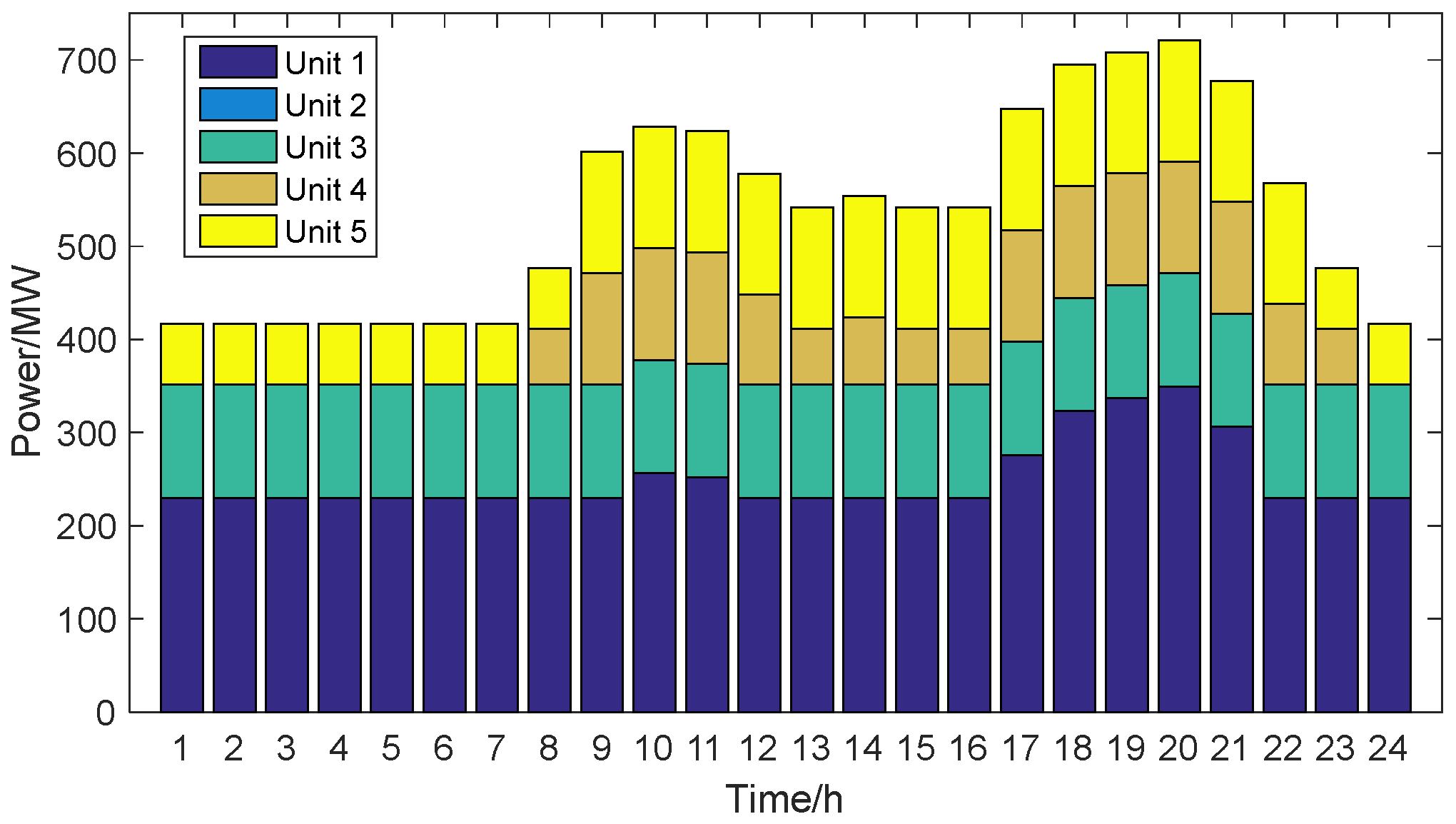
The simulation calculation adopts an improved IEEE 30-node system, including 5 thermal power units connected to nodes 1, 2, 5, 8, and 11 of the system. A 300 MW wind farm and a supporting energy storage power station are connected to node 3 of the system, with an energy storage power of 30 MW and an energy storage capacity of 120 MWh. The energy storage charging and discharging efficiency values are both 0.9. The load curve is shown in Figure 7. In the MATLAB, v. 2015b, software environment, a day-ahead stochastic unit commitment model with wind power forecasting errors was established, and the CPLEX solver was used for solution.

The decision variables for day-ahead stochastic optimization only consider the start-up and stoppage status of thermal power units, and other variables are intermediate variables. The corresponding system operating costs for each scenario are weighted by scenario probabilities and then added up to obtain the total expected system operating costs for day-ahead stochastic unit commitment with wind power forecasting errors. The day-ahead stochastic unit commitment strategies are shown in

Table 1. Day-ahead unit combination.

Time	Unit 1	Unit 2	Unit 3	Unit 4	Unit 5
1	●	○	●	○	●
2	●	○	●	○	●
3	●	○	●	○	●
4	●	○	●	○	●
5	●	○	●	○	●
6	●	○	●	○	●
7	●	○	●	○	●
8	●	○	●	●	●
9	●	○	●	●	●
10	●	○	●	●	●
11	●	○	●	●	●
12	●	○	●	●	●
13	●	○	●	●	●
14	●	○	●	●	●
15	●	○	●	●	●
16	●	○	●	●	●
17	●	○	●	●	●
18	●	○	●	●	●
19	●	○	●	●	●
20	●	○	●	●	●
21	●	○	●	●	●
22	●	○	●	●	●
23	●	○	●	●	●
24	●	○	●	○	●

Notes: “●” indicates that the unit is running, and “○” indicates that the unit is stopped.

.

5.3. Intra-Day Dynamic Optimization Scheduling

On the basis of the unit combination determined in the first stage, in order to verify the effectiveness of the model for intra-day dynamic optimization scheduling, three scheduling modes were set up for comparative analysis in this paper. Modes 1 and 2 optimize the economic efficiency of thermal power and the minimum wind power curtailment, while Mode 3 optimizes the peaking benefits of thermal power units and the wind power benefits. Mode 3 corresponds to the intra-day dynamic optimization mode in this paper. The on-grid benchmark electricity price for thermal power units is 375 RMB/MWh, the on-grid electricity price for wind power is 570 RMB/MWh, the wind power curtailment penalty price is 50 RMB/MWh, the peaking compensation price is 500 RMB/MWh, the average electricity price for the first stage of deep peaking is 200 RMB/MWh, and the average electricity price for the second stage of deep peaking is 500 RMB/MWh. The consistency of intra-day wind power forecast and daily forecast is considered.

Mode 1: thermal power units perform conventional peaking without considering energy storage;

Mode 2: thermal power units perform conventional peaking with consideration of energy storage;

Mode 3: thermal power units perform deep peaking with consideration of energy storage.

5.3.1. Daily Dynamic Optimization Scheduling Result Analysis

By comparing Mode 1 and Mode 2 through

Table 2. Optimization results under different modes. Unit: ten thousand RMB, %.

Mode	Total Cost	Operating Cost of Thermal Power	Cost of Wind Power Curtailment	Wind Curtailment Rate	Peak Regulation Compensation	Profit from Peak Regulation in Thermal Power	Profit from Wind Power
1	52.66	29.48	23.19	10.82%	0.00	0.00	180.10
2	48.56	29.23	19.33	9.02%	0.00	0.00	188.06
3	42.85	32.78	10.06	4.69%	66.77	81.62	205.89

and Figure 8, it can be seen that with the connection of energy storage units under the conventional peak regulation of thermal power units, there is little change in the operating cost of thermal power generation for both modes. However, the total system cost in Mode 2 is reduced by 7.79% compared to Mode 1, and the wind curtailment rate is decreased by 1.8%, which reduces the wind curtailment cost and increases the wind power profit. The operation of energy storage units is beneficial to reducing the overall system operating cost and wind curtailment rate. Despite the minimum technical output limit of thermal power units and the capacity limitation of energy storage units, the wind curtailment situation is still serious for both modes.

By comparing Mode 2 and Mode 3 with the connection of energy storage units, it can be seen that the total system cost in Mode 3 is reduced by 11.76% compared to Mode 2, and the wind curtailment rate is reduced by 4.3%. However, the increase in thermal power generation operating cost due to the deep peak regulation of thermal power units in Mode 3 leads to a 12.16% increase in thermal power generation operating cost compared to Mode 2. The deeper peak regulation of thermal power units further increases the wind power consumption space, reduces the wind curtailment cost, and increases the wind power profit.

Comparing Mode 2 and Mode 3 through Figure 8, Figure 9 and Figure 10, it can be seen that during the severe wind curtailment periods of 1:00–9:00 and 23:00–24:00, Generator 3 was in the second level of deep peak regulation from 1:00–17:00 and 21:00–24:00, while Generator 1 was in the first level of deep peak regulation during 1:00–7:00, 13:00, and 15:00–16:00, and in the second level of deep peak regulation at 8:00 and 23:00. The deep peak regulation period matched the severe wind curtailment period. With the increase in deep peak regulation, the wind farm’s share of peak regulation compensation exceeds the profits gained from participating in deep peak regulation, leading to the wind farm and thermal power units quitting the peak regulation service market transaction.

5.3.2. Optimized Scheduling Results of Energy Storage Systems

By comparing Mode 2 and Mode 3 through Figure 9, Figure 10 and Figure 11, it is apparent that energy storage systems charge during periods of severe wind curtailment and discharge during periods of mild or no wind curtailment to reduce the frequency of charge–discharge cycles as compared to Mode 3. This helps to mitigate wind power curtailment and enhance peak load regulation, providing greater benefits than thermal power generation.

5.3.3. Impact of Different Wind Turbine Capacities on Optimized Scheduling Results

In the electricity market environment, the effectiveness of deep peak shaving and energy storage devices in improving wind power consumption was further verified by gradually increasing the installed capacity of wind farms and analyzing the wind curtailment situation and economic operation of different wind power installed capacities in Mode 3.

As can be seen from

Table 3. Economy under different levels of wind power installed capacity. Unit: RMB, %.

Wind Power Capacity	Total Cost	Cost of Wind Power Curtailment	Profit from Peak Regulation in Thermal Power	Profit from Wind Power
300	428,464	100,622	816,191	2,058,934
350	608,805	305,714	943,887	2,316,773
400	848,603	567,131	1,103,299	2,457,555
450	1,130,392	868,115	1,267,131	2,517,381
500	1,556,436	1,305,584	1,402,545	2,293,938

and Figure 12, as the wind power capacity increases, the wind curtailment rate also increases, with a 22.99% increase in curtailment rate when the installed capacity of wind power increases from 300 MW to 500 MW. The demand for deep peak shaving in thermal power increases, the cost of fuel for deep peak shaving in thermal power increases, and the profit of thermal power peak shaving and the total cost of the system show an increasing trend, while the wind power profit shows a trend of first increasing and then decreasing. Considering all aspects, the installed capacity of wind power in the system should take into account both system aggressiveness and wind curtailment rate, and moderate wind power integration is recommended.

6. Conclusions

In this paper, we have addressed the uncertainty of day-ahead forecasting errors and the auxiliary service constraints of deep peak shaving. We have proposed a two-stage optimized scheduling model for day-ahead and intra-day scheduling and conducted multi-mode case analysis to draw the following conclusions:

Firstly, the scenario-based day-ahead random optimization scheduling approach effectively resolves the trade-off between reserving spare capacity and sacrificing economic efficiency. The optimized unit combination obtained demonstrates universality for various scenarios.

Secondly, the intra-day dynamic economic scheduling, based on the day-ahead random unit combination, includes the auxiliary service constraints of thermal power units participating in deep peak shaving. By enabling both thermal power units and energy storage units to participate in optimized scheduling, the accommodation capacity of wind power is further improved.

Lastly, in the electricity market environment, increasing wind power capacity can enhance the profits of thermal power peak shaving. However, we observed that wind power profits exhibit a trend of initial increase followed by a subsequent decrease as wind power capacity increases. Considering system proactivity and the curtailed wind power rate, it is advisable to moderately install wind power capacity in grid-connected wind farms within the power system.

In conclusion, our study demonstrates the effectiveness of the proposed scheduling model in managing day-ahead uncertainty and enhancing the accommodation of wind power. Future work can focus on further improving the model by considering additional factors, such as demand response and transmission constraints. Additionally, it is important to acknowledge the limitations of our research, such as considering load and renewables uncertainties, which are relevant in reducing costs and avoiding network problems, and will be the focus of further investigation.