Abstract
Research on the power prediction of proton exchange membrane fuel cells (PEMFCs) has garnered considerable attention. Because mainstream computational-fluid-dynamics-based methods are time-consuming, this study aimed to design a data-driven method based on Ridge regression (Ridge) and convolutional neural network (CNN) algorithms that can efficiently predict PEMFC power under uncertain conditions in real-world scenarios and reduce the time consumption. The measured data from a PEMFC test bench (3 kW) were collected as the data source for the model. First, we adopted Ridge to eliminate abnormal samples. Second, we analyzed and selected the variables that have a significant effect on PEMFC power. Moreover, we optimized the model using batch normalization, dropout, Nadam, Swish, and Huber techniques. Finally, the performance of the model was evaluated by combining real datasets and real polarization curves. The experimental results demonstrate that the polarization curves predicted by the CNN-based model agree with the real curves, with a prediction accuracy of approximately 0.96, a prediction time of 1 μs, and an iteration period of less than 1 s per cycle. A comparative analysis shows that the CNN-based model prediction precision was superior to that of other mainstream machine learning algorithms. In real scenarios, the CNN-based model accurately predicts the power of PEMFC.
1. Introduction
Proton exchange membrane fuel cells (PEMFCs) are energy conversion devices that transform chemical energy into electrical energy [1]. Currently, China is vigorously developing hydrogen energy owing to its characteristics of zero pollution, zero noise, high operating efficiency, high power density, and low-temperature operation [1,2,3,4,5], with PEMFCs being an important development direction in fuel cells. PEMFCs use polymer electrolyte membranes (particularly Nafion212) to conduct protons and separate gaseous reactants on both sides of the cathode and anode, making them best suited to replace automotive internal combustion engines. Free from the constraints of the Carnot cycle, the PEMFC, with a power generation efficiency as high as 40–60%, has become one of the main power generation options for distributed generation, portable power sources, and hybrid electric vehicles [6,7,8,9,10]. To improve PEMFC performance, it is essential to develop an accurate model to predict its overall performance and adjust it to improve its operating efficiency.
The performance of a PEMFC is represented by an I–V curve, which is affected by many factors, including operating conditions, material properties, fuel cell dimensions, and physical and electrochemical processes [11,12,13,14,15]. Numerous physical models and techniques have been developed to predict or measure polarization curves [15,16,17,18,19]. PEMFC performance prediction is mainly categorized into two approaches: data- and model-driven [20].
Model-driven approaches include empirical or semi-empirical models that are used to predict PEMFC performance [21,22,23,24,25,26] and include analytical, mechanical, and computational fluid dynamics (CFD) models, which are three-dimensional (3D) physical models. Three-dimensional physical models comprehensively consider the effects of chemical reactions, such as the reaction of kinetics and physical and chemical parameters [27]. To date, numerous approaches based on 3D physical models have been developed to predict PEMFC performance and study the influence of operating conditions [16,17,18,19,28]. Zhang et al. [29] established a 3D non-isothermal dynamic PEMFC model, studied the start-up strategy, and investigated the start-up time and temperature distribution during the start-up process. Xie et al. [30] established a 3D agglomerate PEMFC sub-model of the catalyst layer (CL) by investigating the effect on PEMFC performance through platinum loading and ionophore resistance. An optimal model can render more accurate predictions; however, designing a high-precision physical model for the PEMFC operating environment is a demanding task. This is because, as a problem in conventional CFD modeling, the membrane electrode assembly (MEA) contains complicated transport and electrochemical phases during PEMFC operation [27]. If traditional PEMFC model-driven methods are used, a deep understanding of the process parameters and physicochemical phenomena of the PEMFC is required [8,31], but these vary for different types of fuel cells, making them unsuitable for wide application in other types of fuel cells with different parameters [20]. Researchers should conduct several experiments to improve PEMFC performance and obtain the I–V curve, which is time-consuming and entails significant costs. Despite their capabilities for overall and local PEMFC performance prediction, 3D methods are time-consuming and require massively parallel computing to research microstructural constituents [32,33,34], industrial-scale fuel cells [28,35], and PEMFC stacks [36], as summarized in Table 1.

Table 1.
PEMFC performance prediction based on physical models.
Computational and time costs are typically high in traditional 3D-physical-model-based methods, while predictions using simplified physical models lead to low accuracy [15]. Even for small-scale stacks consisting of 5–10 cells, 3D simulations based on physical models typically require 100–1000 million grid points and days or weeks to predict a steady-state operation [16,17,39]. Wang et al. [40] created a 3D PEMFC model with a CL agglomerate sub-model and constructed a performance database of PEMFCs with various CL compositions. The database was then used to train a data-driven model based on support vector machines (SVMs); the model had a predictive accuracy similar to or higher than that of conventional physical models and was more computationally efficient by several orders of magnitude. Predicting I–V curves takes only a second in a data-driven model but hundreds of hours of processing with a processor in a 3D-physical-model-based approach [15].
In contrast to model-driven approaches, data-driven methods do not require an understanding of the physical–chemical mechanisms and predict the performance based on the measured data obtained during PEMFC operation [20]. Data-driven models, including machine learning (ML) models, do not require prior knowledge and understanding of the complicated transport and electrochemical phases that occur during PEMFC operation, which significantly decreases the difficulty of modeling. Furthermore, ML-based methods excel in computational efficiency, and a data-driven approach can be applied to all aspects of PEMFCs. It has been documented that ML-based methods are effective in predicting aspects of PEMFCs, such as the PEMFC time-series voltage, PEMFC temperature, hydrogen flow, oxygen flow, the lifetime of the PEMFC, the material selection and optimization of membrane electrodes, the degradation of membrane electrodes, the design and optimization of flow channels, PEMFC fault diagnosis, PEMFC system control strategy and optimization, and PEMFC health status management and monitoring. The prediction speed and accuracy of ML-based methods are high, which shows the significant application potential of data-driven methods in PEMFCs. To study PEMFCs, multiple attempts have been made to propose ML-based methods for the replacement of complex 3D physical models. As summarized in Table 2, various ML-based methods have been applied for PEMFC modeling.

Table 2.
ML-based PEMFC modeling.
ML-based models have relatively few parameters and are suitable for small datasets; however, they do not perform well on large datasets, whereas deep learning (DL)-based methods are suitable for large datasets. Although several ML-based models have been proposed to predict the performance of PEMFCs, few DL-based methods have been applied to predict the power of PEMFCs, and the data sources are mostly based on CFD modeling, as summarized in Table 3. It only takes a fraction of a second to predict the power of a PEMFC by applying DL-based methods, and the accuracy is higher. Introducing DL-based methods into PEMFC research can solve complex mechanical problems in traditional physical model methods and significantly improve the efficiency of PEMFC operation, system analysis, and optimization, which reflects their broad research prospects in PEMFCs. Therefore, this study investigated the PEMFC power and optimal model for PEMFC power prediction using DL-based methods.

Table 3.
PEMFC power prediction based on DL methods.
The PEMFC instantaneous power prediction model aims to achieve the best operational performance, optimizing performance on the basis of the power predicted by the model. Transient characteristic variables, such as hydrogen and air flow transients, are input to a model that can predict the transient power of the PEMFC. This research applies to the design and development phase of fuel cells, where the researcher predicts the corresponding power by adjusting the values of any or several different PEMFC characteristic variables. The predicted power is then used to adjust the characteristic variables (i.e., parameters) and eventually adjust the PEMFC parameters within the desired range. This research helps designers to reduce the time cost and iteratively optimize the PEMFC design solution.
This study provides a PEMFC power prediction model based on Ridge and CNN data-driven models, reducing the cost of extensive experiments. The I–V polarization curve was selected as the target for power prediction Further, the influence of 20 characteristic variables on the PEMFC power was analyzed, and 10 characteristic variables with significant influence on the power were selected by using the methods of kernel density estimation (KDE) and heat mapping. Furthermore, DL technologies (including batch normalization and dropout layers) were used to increase the accuracy and generalization capacity of the model, and the model was optimized through the Nadam optimization algorithm, Swish activation function, Huber loss function, etc. There is a lack of actual data on PEMFCs in the previous literature, as most of the data were obtained using methods based on CFD modeling. This study applied measured data from a PEMFC system test bench (3 kW) in the laboratory, which includes 20 PEMFC characteristic variables, such as cell temperature, hydrogen and air flow, and hydrogen and air backpressure, to demonstrate the reliability and applicability of the model in real-world scenarios. In the previous literature, only two or three algorithms were compared for the determination of the optimal model for PEMFC power prediction, and the conclusions were not sufficiently comprehensive. Therefore, we complement the previous literature by comparing and optimizing more than ten mainstream conventional ML, ensemble learning (EL), and DL methods to propose an optimal model for PEMFC power prediction, providing a strong basis for the selection and optimization of the model. It takes days or weeks to predict a point on a polarization curve using mainstream CFD-based methods. Data-driven modeling methods can predict power within 1 μs to reduce the time cost. Trained with real data samples, the model is more suitable for PEMFC power prediction in real scenarios. In this study, the instantaneous power values and performance, represented by the polarization curves of the phenomenon at any point in time and in any spatial state, can be predicted with high speed and accuracy. This study can help designers to reduce the time and cost, and iteratively optimize the PEMFC design solution. The obtained power can also be used for the parameter tuning of fuel cells within the desired range. This study contributes to solving the problem of the difficulty in predicting the instantaneous energy consumption of the fuel and power cell side of PEMFCs.
2. Materials and Methods
2.1. Experimental Data Source
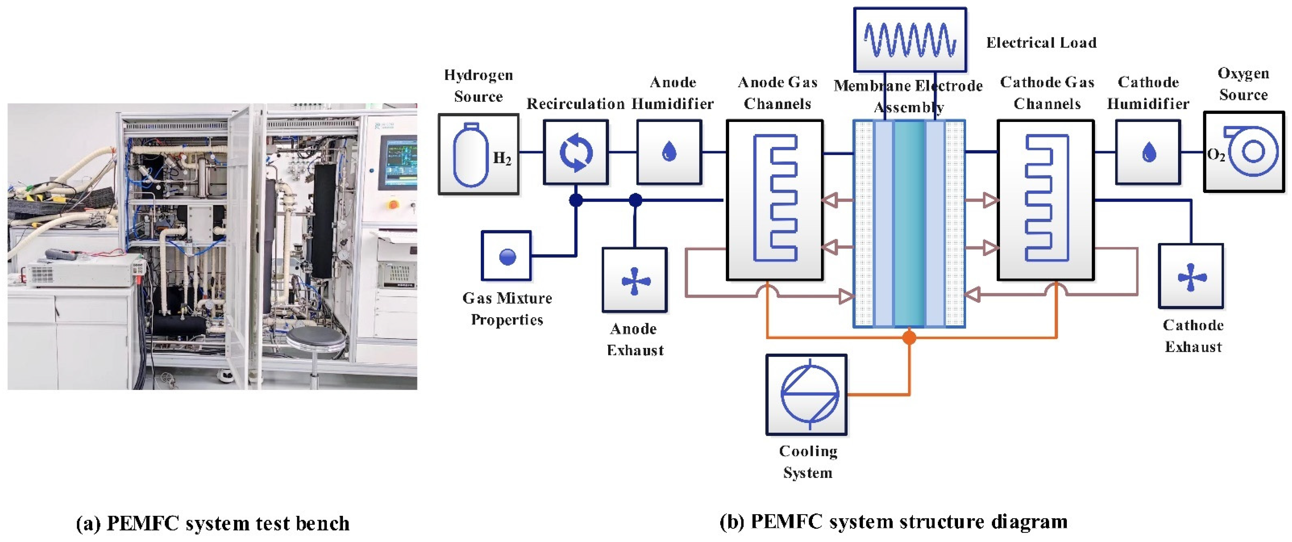
The data in this study are the actual measured data obtained with a PEMFC system test bench (RG220-3 kW, Dalian Rigor New Technology Co., LTD., Dalian, China), as shown in Figure 1a. The power range of the RG220 was 1.5~5 kW. The main purpose of the test bench was performance evaluation, activation, lifetime testing, and quality inspection of PEMFCs. The real-time monitoring interface of the PEMFC system test bench monitors the temperature, gas pressure, and gas flow of the PEMFC in real time. This experiment was conducted on a 3 kW PEMFC system test bench to feed hydrogen and air into the control system of the test bench to adjust the pressure, temperature, backpressure, stoichiometric ratio, flow rates of hydrogen and air, PEMFC temperature, and the real-time stack power obtained from the magnitude of the current. The test bench collected data every second. The operating parameters of the test bench were as follows: the relative humidity was 100%, the operating temperature was room temperature, the time interval of sampling was 1 s, and the stack power was 3 kW. Figure 1b shows the PEMFC test bench system structure. The PEMFC parameters are listed in Table 4.
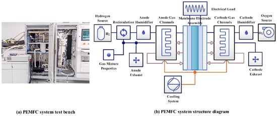
Figure 1.
PEMFC system test bench and corresponding structure diagram.

Table 4.
PEMFC material composition.
The precision and accuracy of the dispensed liquid volume has a vital role in the overall efficiency of industrial processes. Meera et al. [54] proposed an automated accurate liquid transfer system that can replace the traditional unstable flow meters and expensive flow sensors used in the industry. This non-contact system improved the overall efficiency of the liquid transfer process in a remarkably cost-effective manner and has applicability in PEMFC systems.
This study used Python programming language to operate MXNet in the DL framework in the environment configuration of RTX2060. The datasets obtained by the experimental methods of this system test bench include physical and chemical parameters influencing the PEMFC and operational parameters during the test. Because the polarization curves can represent the power of the PEMFC, we employed the polarization curve as the main performance index. All datasets were randomly divided into training and test sets in a ratio of 8:2. Table 5 lists the statistical information of the training dataset, including the number of samples (Count), mean values (Mean), standard deviations (Std), minimum (Min), maximum (Max), lower quartile (25%), median (50%), and upper quartile of the data (75%). The training set had 10,988 samples and 20 characteristic variables (V0–V19) that affect the power of the PEMFC stack, with stack power set as Target, that is, the target variable predicted by the model, where the variable types were all numerical. Table 6 lists the statistical information of the test dataset. Similarly, the test set had 2748 samples with 20 characteristic variables (V0–V19), which were all numerical. None of these characteristic variables required a control variable. There was no need to fix one characteristic variable and adjust the rest. The corresponding power was obtained by randomly adjusting the values of the characteristic variables and inputting them into the model, implying the wide applicability of the model. Only 20 characteristic variables are mentioned here, and details about the analysis of the effects of more characteristic variables on the PEMFC are given in the Feature Transformation section (2).

Table 5.
Statistical information of the training set data.

Table 6.
Statistical information of the test set data.
2.2. Experimental Algorithms
Because each algorithm has its own characteristics, we compared a variety of mainstream ML algorithms to make the optimal model more convincing. We used mainstream algorithms, including traditional ML, EL, and DL. Among them, the ML algorithms include linear regression (LR), K-Nearest Neighbor Regression (KNN), Decision Tree (DT), Elastic Net Regression (Elastic Net), Support Vector Regression (SVR), Lasso regression (Lasso), and Ridge; EL algorithms include Random Forest regression (RF), Extreme Gradient Boosting Regression (XGB), Gradient Boosting Regression (GBR), and AdaBoost regressor (AdaBoost); and DL algorithms include CNN and feedforward neural network (FFN).
In deep learning, ANN is one of the most basic neural networks and other neural networks are improvements of ANN structure. ANN consists of a number of interconnected nodes, each node represents the output function of the activation function and the connection between two nodes represents the weights. The output of the networks depends on the connections, weights and activation functions [55]. ANN inspired by information processing in the human brain are also an advanced technique. Salp Swarm Algorithm (SSA) is a metaheuristic algorithm on nature that solves optimization problems by simulating their behavior in nature. Soleimani, S. et al [56] chose the SSA embedded ANN (ANN-SSA) to obtain the least squares sum of errors and investigated its application in predicting the dissolution rate.
Among the mainstream DL algorithms, improved recurrent neural network (RNN)-based algorithms, such as Gated Recurrent Unit (GRU) and long short-term memory (LSTM), have evident advantages for application in predicting time series; however, the iteration speed per cycle is slow. Conversely, the iteration speed of CNN- and FFN-based algorithms is faster than that of RNN-based algorithms; hence, FFN- and CNN-based algorithms were chosen for comparison among DL algorithms.
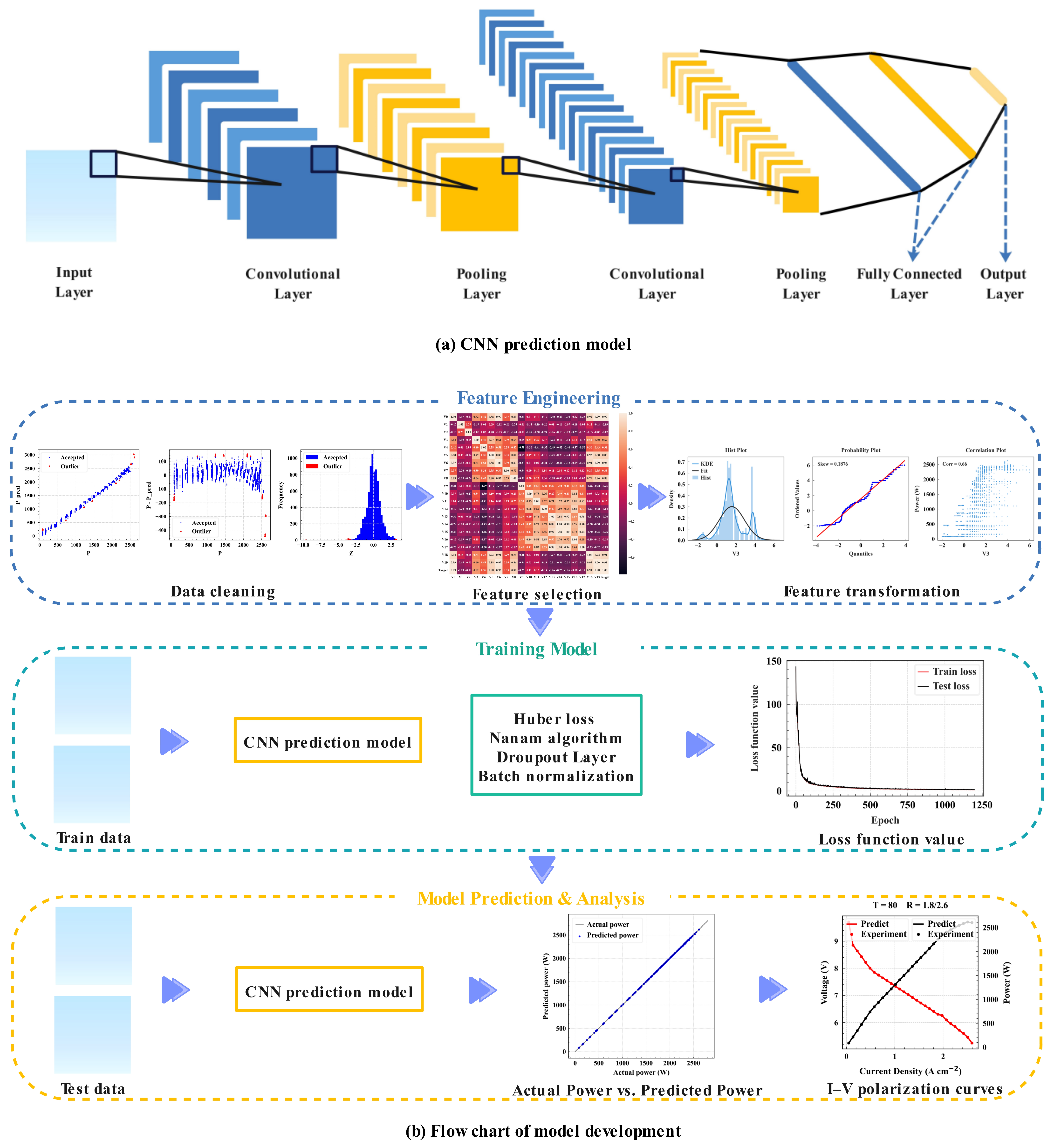
CNN is one of the mainstream DL algorithms with a strong performance in the fields of image recognition and text data prediction. It decreases the complexity of the neural network through three strategies: local receptive field, weight sharing, and down-sampling. Owing to the parameter sharing and sparse connections of the weight-sharing network structure, fewer weight and bias parameters are present in the convolutional layer, reducing the model complexity. The local connection of CNN ensures that the acquired convolution kernel is the most responsive to the local spatial pattern of the input. CNN can learn corresponding features from several input samples, which avoids the complicated feature extraction process. Because FFN is a fully connected layer structure with more parameters, it requires a considerable amount of storage and computational space. The redundancy problem of parameters makes fully connected neural networks less likely to be applied in complex scenarios. Compared with FFN, CNNs are sparsely connected structures, which reduce the complexity of the model and allow it to iterate faster. One-dimensional CNN can also predict time-series data. Compared with one-dimensional CNN, the model structure of 2D CNN accelerates the training speed. Therefore, we adopted a 2D CNN, whose structure is shown in Figure 2a, and the convolution process can be expressed by Formula (1):
where represents the output features of the v-th channel in the convolutional layer l, denotes the weight parameters of the convolutional layer l, and is the bias value. Activation functions were used to implement nonlinear projections of neuron inputs. In this study, the application process of the Swish activation function can be represented as in (2), in which represents the output features of the j-th channel in the convolutional layer l.
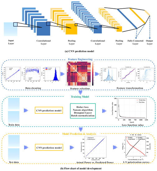
Figure 2.
Development of the prediction model.
2.3. Model Evaluation Index
To validate the reliability of the experimental results, six commonly used indicators were chosen to assess the performance of the prediction model: MSE, RMSE, MAE, MAPE, RAE and R2. In the formulas below, denotes the predicted value, denotes the actual value, and represents the average actual value. The value of R2 ranges from 0 to 1, where 0 indicates no correlation, and 1 indicates a perfect positive correlation. RMSE represents the error between the actual and predicted values. The smaller the values of MSE, RMSE, MAE, MAPE, and RAE, and the closer the value of R2 is to one, the better the performance of the model.
3. Theory and Calculations
3.1. Development of the Prediction Model
This section illustrates the PEMFC power prediction model. The flow chart of the development of the CNN-based prediction model is illustrated in Figure 2b, which contains the following stages: feature engineering, model training, and model prediction. Feature engineering was performed on the sample datasets for higher prediction precision and a faster convergence speed of model training. Feature engineering includes the processing of abnormal samples in data cleaning, feature selection, feature transformation, and the provision of optimized training samples for prediction models. Thereafter, the training process of the model was performed. With the dropout layer and BN techniques, the generalization ability of the model was improved, and the model was optimized with the Huber loss function, Swish activation function, and Nadam optimization algorithm. Finally, the prediction model was assessed on actual datasets with six commonly used evaluation indicators: Mean Absolute Percent Error (MAPE), Determination Coefficient (R2), Mean Absolute Error (MAE), Root Mean Square Error (RMSE), Relative Absolute Error (RAE), and Mean Square Error (MSE).
3.1.1. Feature Engineering
This section analyzes the critical characteristic variables that influence the PEMFC power. Before training the model, feature engineering was performed for the dataset input to the prediction model. This helps to accelerate the training speed of the model and enhance the accuracy and generalization ability of the model.
Data Cleaning
Missing values affect the performance and accuracy of a model. It is observed from Table 5 that there were no missing values in the training set; hence, no missing value processing was required. We applied the measured data from the PEMFC test bench, which collects data once per second. PEMFC power is affected by 20 characteristic variables. Once the current or pressure is adjusted, the PEMFC control system equipment cannot respond quickly, and the unstable power at the beginning will cause the power to generate abnormal samples. The samples required in this study were steady-state power; hence, these abnormal samples did not need to be detected. If these abnormal samples are not removed, most algorithms cannot identify or avoid the influence of these samples on model parameters. All training data samples, including a few abnormal samples, have the same degree of impact on the final model parameters; hence, the impact of abnormal samples on the model cannot be identified during training, leading to the low prediction accuracy of the model (prediction results will be biased toward abnormal samples). Therefore, it is necessary to remove abnormal samples.
Because Ridge is significantly affected by abnormal samples in the datasets, abnormal samples were excluded from the data used for Ridge predictions, and the remaining samples were input into the model, which effectively reduced the time cost in the presence of a large amount of data. Ridge adds a regularization item to the loss function in the model iteration process and reduces the impact of abnormal samples on model parameters by setting the regularization strength. The greater the regularization strength, the stronger the generalization ability, which limits the matching of model parameters to abnormal samples and biases the prediction results toward normal samples, thereby improving the fitting precision of the model for most normal samples. To avoid the impact of outliers on the prediction results, Ridge reduces the weight of abnormal samples in the calculation.
Figure 3 shows the Ridge model on the training set, in which “Outlier” indicates an abnormal value of power, and “Accepted” represents normal power. The parameter of the Ridge model was set to sigma = 3. Figure 3a is the scatterplot representing the actual power (P) and predicted power (P_pred). Figure 3b shows the residual of the actual power (P) versus the predicted and actual power (P-P_pred). Figure 3c presents the residuals of the predicted and actual power of the model and the frequency (vertical axis: Frequency) falling in the intervals on the Z axis (Z = (resid-mean_resid)/(std_resid). On the horizontal axis Z, resid represents the residual of the predicted power and actual power, mean_resid is the mean value of the residuals of the predicted power and actual power, and std_resid denotes the variance of the residuals of the predicted and actual power. Setting the Ridge model parameter sigma = 3 indicates that samples with absolute values of residuals of predicted and actual power exceeding 3 (absolute value of Z exceeding 3) are considered abnormal samples.

Figure 3.
Ridge model on the training set. (a) The actual power and predicted power. (b) The residual of the actual power versus the predicted and actual power. (c) The residuals of the predicted and actual power of the model and the frequency.
R2, MSE, RMSE, MAE, MAPE, and RAE of the Ridge model on the training set were 0.9968, 2076.3202, 45.5666, 33.4631, 0.0617, and 0.0461, respectively. Seventy-three groups of abnormal samples were removed, and the remaining samples were input into the model for training. Similarly, for the Ridge model on the test set, R2, RMSE, MSE, MAE, MAPE, and RAE were 0.9963, 49.3830, 2438.6881, 37.9738, 0.0670, and 0.0514, respectively. Twelve groups of abnormal samples were removed.
Feature Selection
This section analyzes the impact of important characteristic variables on the PEMFC and the reasons for selecting the characteristic variables. The objective of this analysis is to choose the features that are necessary for the prediction model to attain high performance (accuracy).
- (1)
- KDE Distribution
Based on the distributions of all characteristic variables in the training and test sets in the KDE distribution graph, those with inconsistent distributions between the two datasets were removed to improve the prediction accuracy of the model. Figure S1 (in Supplementary Material) shows that because there was a large quantity of data samples in the two sets and their distributions in the two datasets were relatively consistent, it was unnecessary to exclude any characteristic variables.
- (2)
- PEMFC Characteristic Variable Analysis
The main influencing factors of the PEMFC are categorized into two types: operating and physicochemical parameters. In this study, the physicochemical parameters were kept constant, as summarized in Table 4. Among them, the backpressure of oxygen is an important operating parameter, which, together with the oxygen flow rate, is related to the stack power density, voltage–current characteristic, and voltage [57]. Raising the backpressure facilitates a rise in the partial pressure of the reactant gases and the electrical potential of the PEMFC, which is conducive to improving the performance of the PEMFC. The cell temperature is another important operating parameter that significantly impacts PEMFC performance. As the temperature rises, the cell performance improves within a certain range. The ohmic resistance of the electrolyte drops as the temperature rises, resulting in a lower internal resistance of the cell and a higher mass transfer rate. However, the PEMFC’s working temperature is limited by the water vapor pressure in the proton exchange membrane. If the temperature is high, the dehydration of the membrane leads to compromised ion conductivity.
The method in this study predicts the transient power of the PEMFC and polarization curves instead of the dynamically varying power. Therefore, transient data of the characteristic variables should be collected when the test bench reaches a steady state. Because the reactants are consumed along the length of the gas flow channels, which results in a change in the potential from the inlet to the outlet, the current density is not uniform. However, it does not influence the results predicted by the model. Because the test bench collects data once per second, when it is adjusted to a steady state, the data of the current density are also steady and remain almost unchanged. The inlet flow rate is variable and should not be controlled to match the consumption of the reactants because no matter how much the inlet flow rate changes or how much of a reactant is consumed, the data of these variables are input to the model, which predicts the results based on these available data. These are the advantages of AI-based models. In this study, the influence of critical characteristics on the PEMFC was adequately analyzed, for example, liquid condensation and critical limits for liquid water slug formation and movement, the variation in membrane resistance with local water activity and temperature, and the effect of gravity on liquid slug formation in the fuel cell flow channels. However, these characteristics have significantly little influence on the PEMFC power, and their performance influences certain critical characteristic variables (V0–V19). We selected the critical characteristic variables connected with the PEMFC stack: these variables have a significant influence on the stack. We simply considered the precision and training speed of the model in a real situation. Inputting too many characteristic variables into the model is not conducive to the training of the model; hence, they have minimal influence on the prediction results, and therefore, only the more significant characteristic variables (V0–V19) were analyzed.
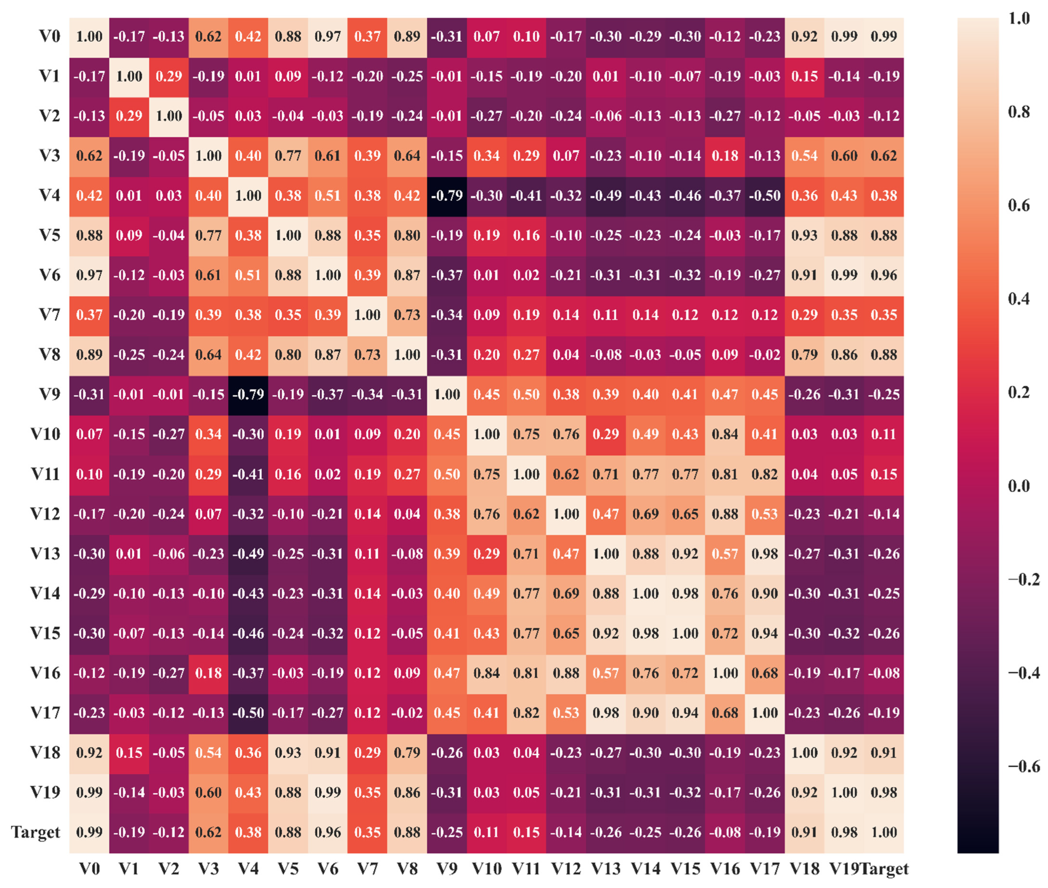
We investigated the impact of the 20 operating parameters in Table 5 on the target variable. If too many characteristic variables are input, the model will become complicated, and its performance will decrease. Therefore, the heat map method was adopted to analyze the correlations between characteristic variables V0–V19 and the correlations between these variables and the target variable. The characteristic variables that significantly impact the power of the PEMFC were screened out based on their correlation coefficients. It is observed in Figure 4 that the characteristic variables with a correlation coefficient greater than 0.3 with the target variable were V0, V3, V4, V5, V6, V8, V18, and V19. V8 indicates the cell temperature.
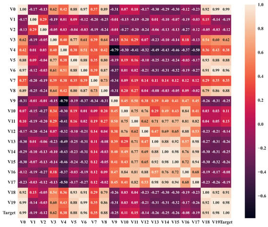
Figure 4.
PEMFC correlation matrix.
The current was adjusted from small to large for each run on the test bench to enable the PEMFC to reach its maximum power when it was stable. Therefore, most of the data samples were concentrated below 75 °C, that is, in the range where the current density was low, leading to small correlation coefficients of V1 and V2 with the Target. This is because there are three types of polarization in the PEMFC: concentration, ohmic, and activation polarization. Activation polarization plays a major role, while the stoichiometric ratio has a limited influence on the stack performance at low current densities [58]. Concentration polarization plays a central role, and the stoichiometric ratio has a greater impact on the stack performance at high current densities. The larger the stoichiometric ratio, the higher the voltage. In actual reactions, it is necessary to add excess air to overcome the limitation of mass transport on the cathode side. The stoichiometric ratio is an important PEMFC parameter. A larger stoichiometric ratio increases the reaction rate of air and hydrogen within a certain range. Large amounts of unreacted air and hydrogen in the flow channel have a satisfactory purging effect on liquid water, and the speed of the reaction to generate water is fast, thereby making the PEMFC’s performance preferable. The stacks should work at a higher stoichiometric ratio at high currents. In consideration of the future applicability of the model, the characteristic variables V1 and V2 were added. Finally, 10 characteristic variables related to the Target were selected, namely, V0, V1, V2, V3, V4, V5, V6, V8, V18, and V19, while the other characteristic variables that were less relevant to the Target were excluded.
Feature Transformation
The objective of the process described in this section is to transform necessary features, reduce the complexity of the model, and increase the performance of the prediction model.
- (1)
- Z-Score Standardization
The data need to be normalized before being fed into the model to scale the data to the specified interval. As the model presumes a corresponding data distribution, it eliminates the influence of dimensions or values on the calculation results. Additionally, it can accelerate the gradient descent to obtain the optimal solution during model training, which improves the precision of the prediction results. Because the current range in the datasets in this study was 0–500 A, the backpressure range was 0–1 MPa, the maximum difference between the current and back pressure was vast, and the dataset was complicated by plenty of outliers and noise in the data, Z-score standardization was preferable to avoid the indirect influence of outliers and extreme values through centralization. The formula is as follows:
where represents the sample, denotes the standard deviation of the sample, denotes the mean of the sample, and denotes the sample after normalization.
- (2)
- Yeo–Johnson Transformation
Owing to the influence of the uneven distribution of variable values on the model’s performance, there were samples with zero or negative values in the data after normalization. Therefore, the Yeo–Johnson transformation was used to convert the value range of variables, reduce the heteroskedasticity of random variables, and amplify their normality, which mitigates the correlation between unobservable errors and predictive variables to a certain extent, such that the shape of the probability density function is approximated to a normal distribution. Consequently, the model satisfies linearity, normality, independence, and homogeneity of variance, which facilitates the fitting of linear models and feature correlation analysis, increasing the training speed of the model.
Histograms of the characteristic variable V3 are given in Figure S2a,b to evaluate the conformity of the original and transformed data to a normal distribution. Figure S2(a1–a3) show the histograms before the Yeo–Johnson transformation. Figure S2(a1) shows the probability density distribution of the original data of V3, which is used to evaluate the conformity of the variable to a normal distribution. It can be observed in the figure that the original data of V3 did not follow a normal distribution. Figure S2(a2) is a Q-Q diagram, that is, a graph comparing the quantiles of the original data and those of a normal distribution. If the original data fit a normal distribution, all the points would fall on a straight diagonal line. If the data distribution did not follow a diagonal line, the data were subsequently converted using the Yeo–Johnson transformation. The closer the blue points are to the red line, the better the fit. The skew represents the asymmetry of the data distribution, and the closer the skew is to zero, the better the fit. The skew of V3 was −1.7805. Figure S2(a3) shows the correlation coefficient diagram, where Corr is the correlation coefficient used to describe the degree of correlation between the two-dimensional random variable V3 and the two components of the Target. The correlation coefficient is within [−1, 1], and the closer Corr is to ±1, the stronger the correlation; the closer it is to zero, the weaker the correlation. Among them, the initial Corr of V3 was 0.62.
Figure S2(b1–b3) illustrate the probability density distribution diagram, Q-Q diagram, and correlation coefficient diagram of the characteristic variable V3 after the Yeo–Johnson transformation, respectively. The probability density of the original feature data approximated a normal distribution after the Yeo–Johnson transformation. The asymmetry was reduced from −1.7805 to 0.1876, and the correlation coefficient increased from 0.62 to 0.66. Similarly, Table 7 lists the coefficients of all characteristic variables before and after the Yeo–Johnson transformation. After the Yeo–Johnson transformation, the asymmetry of all characteristic variables was lower, whereas the correlation coefficients were higher.

Table 7.
Yeo–Johnson transformation of all variables.
- (3)
- Feature Dimension Reduction
In the training dataset, because of the large correlation coefficients between each characteristic variable and other characteristic variables, the possible severe effects of collinearity may lead to inaccurate prediction results from the model. The variance inflation factor (VIF), a measurement of the severity of multicollinearity in multiple linear regression models, expresses the ratio of the variance of the regression coefficients to that when the independent variables are assumed to be nonlinearly correlated. Multicollinearity analysis was performed on 10 characteristic variables in the VIF matrix. Table S1 (in Supplementary Material) indicates that the correlation coefficients between V0, V6, V19, and other variables were relatively large. Principal component analysis (PCA) was conducted to eliminate multicollinearity and reduce dimensionality.
Feature dimension reduction can reduce errors caused by redundant information, thereby enhancing the precision of model recognition. PCA maps high-dimensional data to a low-dimensional space through a linear projection and expects the largest variance of data in the projected dimension to retain more original data point features with fewer data dimensions. After PCA dimension reduction, the number of principal components remained 10. The VIF of each characteristic variable was within one after dimensionality reduction.
3.1.2. Prediction Model
Structure of the Prediction Model
Figure 5b depicts the structure of the 2D-CNN model used in this study, which incorporated DL techniques, including dropout and BN. Additionally, the model was optimized with the Huber loss function, Nadam optimization algorithm, and Swish activation function, which improved the computing performance.
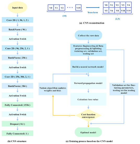
Figure 5.
CNN model.
In this study, data reconstruction was conducted to convert the training dataset into a standard input format for a CNN-based prediction model. As shown in Figure 5a, the data of 10 characteristic variables were input into the model to convert these sequence data into an image format.
- (1)
- Activation Function
The activation function is an important part of the DL model because it has a significant effect on the precision of the prediction results and the computational efficiency of the training process. Different activation functions and initialization methods significantly influence the convergence speed of model training. In the previous literature, the ReLU function was used as the CNN activation function, but it has some shortcomings. For instance, when the input is negative, the gradient of the ReLU function is zero, whereby the neuron output can only be zero. To overcome such shortcomings, the Swish function was used as the activation function. In this study, FFN and CNN employed the He initialization method and Swish activation function.
- (2)
- Loss Functions
The presence of power outliers in the training set has a significant effect on the prediction results of the model in this study. The more the outliers, the lower the accuracy of the model. Hence, the Huber loss function was adopted to impose smaller penalty terms on the outliers.
The MSE function is highly sensitive to outliers. Models significantly affected by outliers are more inclined to accept bigger penalty terms and give them greater weights while ignoring the role of smaller terms. The problem of a possible gradient explosion caused by outliers is unavoidable owing to the predictive effect of other normal data, leading to the compromised overall performance of the model. Compared to MSE, the MAE function is not sensitive to outliers, and its robustness is better. The gradient in MAE training is often large and equal in most cases. Furthermore, it is continuous at point zero but not derivable. Basically, the gradient is large even for small loss values, reducing the learning rate of the model. Meanwhile, it also causes a missed global minimum value at the end of the gradient descent, which is not beneficial to the convergence of the function and model learning.
The Huber function combines the advantages of the MSE and MAE functions. The function is smooth in [−1, 1], which solves the problem of the roughness of the MAE function, realizes constant derivation, and has a faster convergence speed than that of MAE. In the [−∞, 1) (1, +∞] interval, the problem of the gradient explosion of outliers that may arise in the MSE function is solved, the oversensitivity to outliers is weakened, and the gradient variation is relatively small. When || > , the gradient is always approximated to , ensuring that the model updates parameters at a faster speed. When || ≤ , the gradient gradually declines, which also guarantees that the model can obtain the global optimal value more accurately. When = 5, the power fluctuates with the influence of various control system parameters and operating parameters within the range of 5 W. Here, is the real value, and is the predicted value.
Optimization Model
- (1)
- Optimization Algorithms
Nesterov-accelerated adaptive moment estimation (Nadam) is an improvement based on adaptive moment estimation (Adam). With stronger constraints on the learning rate, it can improve the performance of the optimization algorithm. The formula for Nadam is as follows:
where and are the first- and second-order moment estimations of the gradient, respectively, which can be regarded as the estimation of the expectations . and are corrections of and , respectively, which can be approximated as an unbiased estimation of the expectations. represents the exponential decay average of historical squared gradients, and history denotes the exponential decay average of gradients.
- (2)
- Dropout layer
The purpose of the dropout layer is to prevent the model from overfitting. It was only applied in the training process of the model. During the training process of the model, some neurons’ activation values were randomly allowed to be zero; that is, these neurons were dropped. During the testing phase of the model, all neurons were kept in a working state, while the dropout layer was no longer applied in this process. The value of dropout can be determined from the validation set.
- (3)
- Batch Normalization
Batch normalization (BN) is conducive to accelerating the training process of DL prediction models [59]. Following the BN of the input samples, the output data of each layer were transformed into a normal distribution, such that the subsequent network layers could adapt to the data characteristics with different distributions without learning the data distribution of the previous layer. The process after BN is equivalent to the application of the linear part of the S-type activation function, which can alleviate the problem of the vanishing gradient in the backpropagation of the S-type activation function. BN accelerates the convergence of the model with a high learning rate for initialization and a fast learning rate decay to enhance the training speed of the model and the generalization ability of the network. BN can be expressed as follows:
In this case, y represents the output features, m represents the number of samples in the batch, and is a small constant. and denote the mean value and the standard deviation of all samples in this batch, respectively. and denote shift and scale parameters, respectively, which are obtained by model learning.
- (4)
- Computing Performance Improvement
MXNet integrates the advantages of both imperative and symbolic programming in hybrid programming. In this study, the neural network model constructed in the HybridSequential class was used to call the hybridize function to convert the imperative program into a symbolic program to maximize efficiency and performance. MXNet improved the computing performance of the model through asynchronous computing and automatic parallel computing on the CPU and GPU.
3.1.3. Model Training Process
Figure 5c shows the training flow chart based on the CNN model. The weight parameters of this model were optimized using Nadam (see the Optimization Model section for details). The weight parameters on the training dataset were continuously updated in gradient descent. The loss function values of the error between the actual target value and the predicted output of the model were calculated with the minimum error using the Huber loss function (see the Structure of the Prediction Model section for details). According to the values of the loss function, the Nadam optimizer constantly updated the weight parameters of the model. The purpose of this research is to accurately predict data with CNN-based models. To evaluate the generality of the model, the data were categorized into training and validation sets. During the training process, the training errors were measured based on the training dataset. The model performance was evaluated based on the validation errors computed on the validation dataset, where the dropout method was chosen to avoid model overfitting.
4. Results and Discussion
4.1. Model Parameters
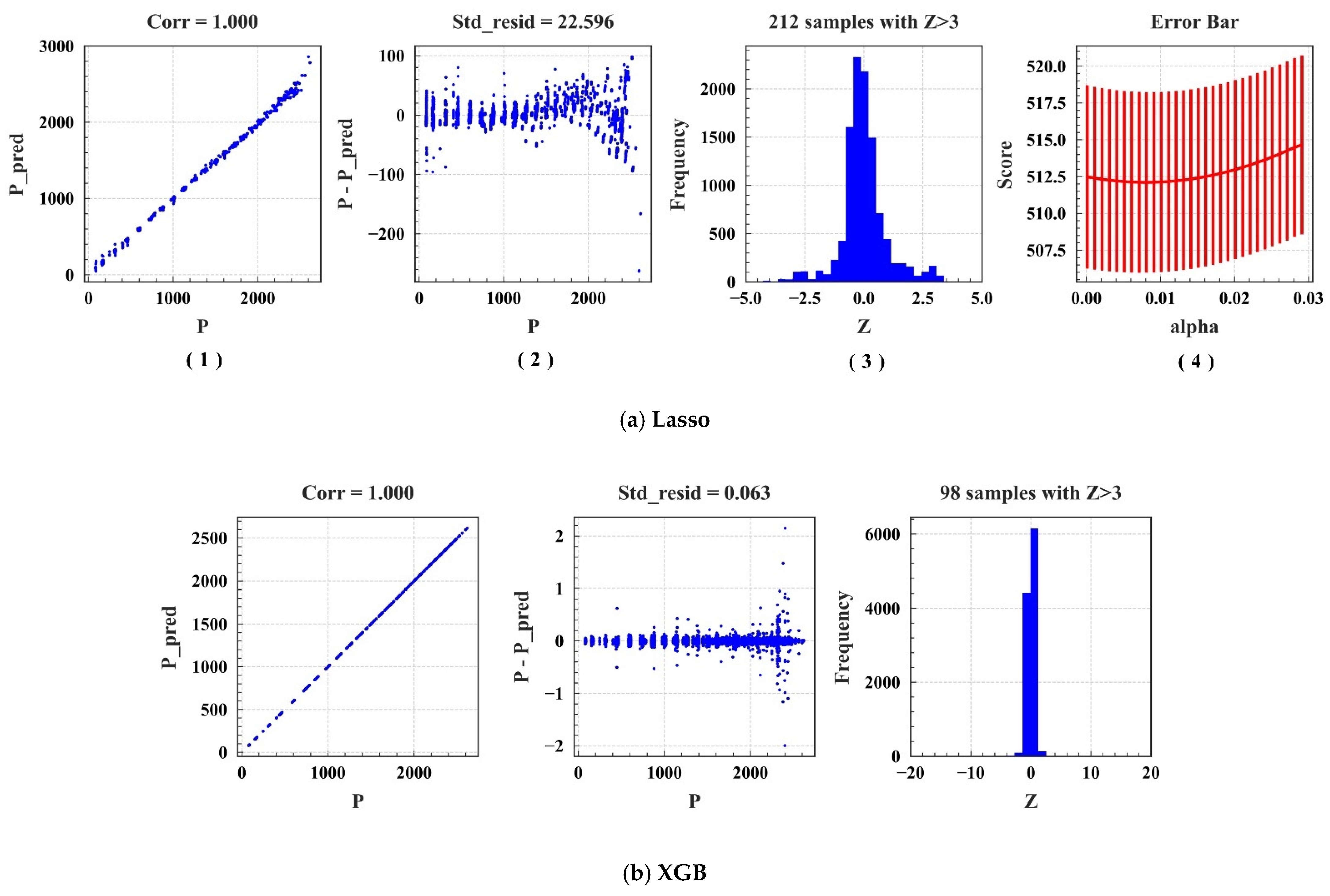
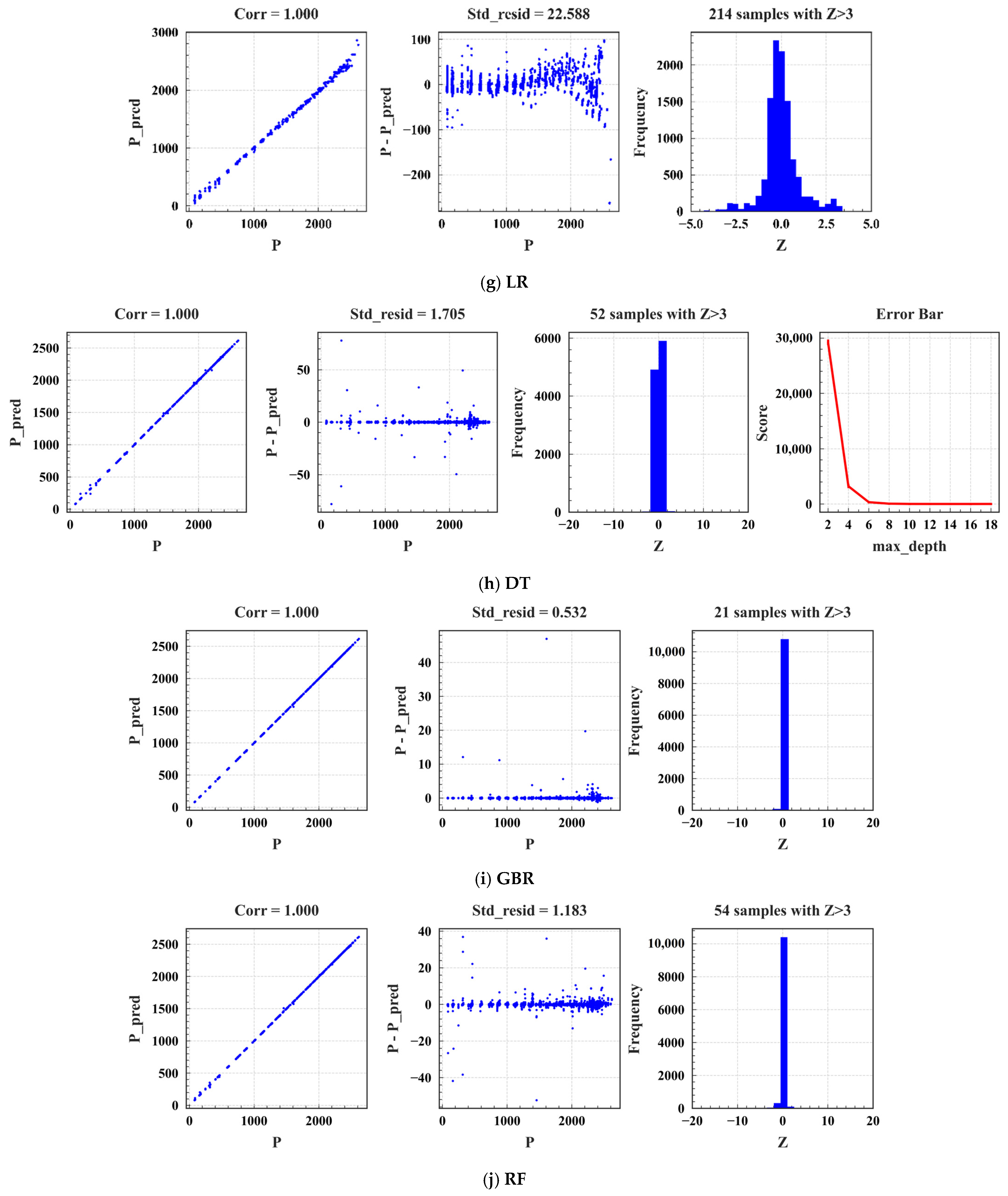
Taking a part of the data in the training set as the cross-validation set, the optimal parameters of each model were found with 5-fold cross-validation and a grid search algorithm. Figure 6 represents the process of tuning parameters for traditional ML and EL. The prediction results of traditional ML models (Lasso) are shown in Figure 6a. As shown in Figure 6(a1), Lasso is the scatter plot of actual power (P) and predicted power (P_pred), where Corr is the correlation, and the closer it is to one, the better. The Corr of the model in this study was one, indicating a strong correlation. Figure 6(a2) shows the scatter plot of the residuals of the actual power, the predicted power (P- P_pred), and the real value (P), in which Std_resid represents the variance; the smaller it is, the more stable the model. There was a big deviation from the predicted value around P = 2500. In addition, the variance was 22.596, indicating that the model was unstable. Figure 6(a3) shows the residuals of the predicted and actual power of the model and the frequency falling in the intervals on the axis Z (Z = (Resid-Mean_Resid)/Std_Resid). On the horizontal axis Z, Resid represents the residual of predicted and actual power, Mean_Resid denotes the average residual of predicted and actual power, and Std_Resid denotes their variance. A total of 212 samples with Z > 3 indicate that the residual error between P_pred and P is greater than three times the standard deviation. The smaller the value, the better, whereas a larger value indicates that some samples in the prediction have a large deviation. Z = 212 means that this model does not have a good tolerance for data with severe deviations. Figure 6(a4) is the error bar diagram of the Lasso model parameters (alpha) and the evaluation indicator MSE (vertical axis: Score). With the increase in alpha, the value of the evaluation indicator score initially decreased and subsequently increased, and the variance of the model gradually increased. Similarly, the prediction results of EL models (XGB) are shown in Figure 6b. Because the EL models have multiple parameters, the error bar graph is not displayed. Tables S2 and S3 summarize the prediction results of traditional ML and EL models, respectively. “Score” represents the model score, where the model scoring standard is the evaluation indicator MSE, with CV_Mean representing the MSE average error of the 5-fold cross-validation set and CV_Std denoting the average variance of the 5-fold cross-validation set. Tables S2 and S3 show that models based on traditional ML have poor stability, while the stability and inclusiveness of EL models are generally better than those of traditional ML. The model stability of XGB and AdaBoost is better. Thus, Tables S4 and S5 are provided to represent the main parameters of the traditional ML and EL models in the cross-validation model, respectively. Similarly, Table S6 shows the optimal parameters of DL models.
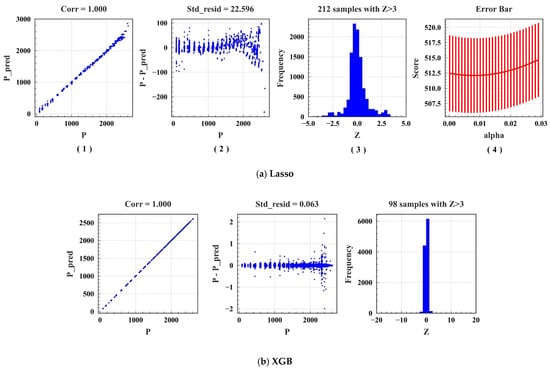
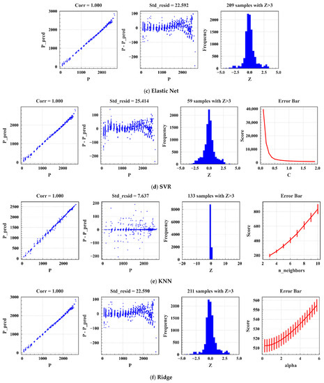
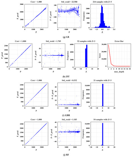

Figure 6.
Prediction effect of the model.
4.2. Model Evaluation
After being adjusted to the optimal parameters, the model was tested for its generalization ability on the test set. Table 8 summarizes the prediction results of traditional ML methods. The large values of the six evaluation indicators do not mean that the performance of the model is unsatisfactory, as it should be analyzed in the actual situation. Because we applied the measured data from the PEMFC system test bench in the laboratory, as shown in Figure 1a, the power fluctuates with the influence of various control systems and operating parameters within the range of 5 W. Therefore, the error between the predicted and actual power is normal in this range. Clearly, traditional ML models have low prediction accuracy and are unsuitable for PEMFC power prediction. This is because traditional ML models are simple and have few parameters, which are unsuitable for predicting large sample sizes and thus not suitable for predicting PEMFC power in this study. Table 9 summarizes the prediction results of EL models, among which the performance of XGB, an improved GBDT-based algorithm, is better. Table 10 also summarizes the prediction results of DL models. Among them, the CNN model has the highest accuracy, where the six evaluation indicators are optimal, with the shortest training time being only 0.7 s for one iteration. Therefore, the CNN model better predicts the power of the PEMFC.

Table 8.
Prediction results of traditional ML models.

Table 9.
Prediction results of EL models.

Table 10.
Prediction results of DL models.
Figure 7a–c show the error curve predicted based on the CNN model, where “Epoch” represents the iteration cycle, “Loss function value” denotes the prediction error of the Huber loss function, “Test” is the test set error, and “Train” denotes the training set error. Applying the parameters in Tables S4–S6, the error curve of the model prediction is divided into three stages. In the first stage, if a small learning rate is used, the gradient decreases slowly and requires many iterations, which is significantly time-consuming. Therefore, we first set a larger learning rate for iteration such that the model gradient decreases rapidly. In the second stage, the error of the model was reduced to a certain range, using a slightly smaller learning rate than in the first stage to prevent the model from skipping the global optimal solution and falling into a local optimal solution. In the third stage, if a larger learning rate is used, the error curve fluctuates a lot. The prediction results are likely to fluctuate around the global optimum, resulting in inaccurate prediction results. Therefore, a smaller learning rate should be used to obtain more accurate results. Figure 7a shows the error curve of the first stage. The model parameters for this stage were set to learning_rate1 = 0.001, epochs1 = 1200, and weight_decay1 = 0.000000001. Figure 7b shows the error curve of the second stage. The model parameters for this stage were set to learning_rate2 = 0.0006, epochs2 = 1200, and weight_decay2 = 0.0000000001. Figure 7c shows the error curve of the third stage. The model parameters for this stage were set to learning_rate3 = 0.00006, epochs3 = 1500, and weight_decay3 = 0.0000000001. It is observed in the figure that the error of the Huber loss function was minimized at approximately 3900 cycles with the increase in the iteration cycle of the model, reaching final errors of Train = 0.31 and Test = 0.56.
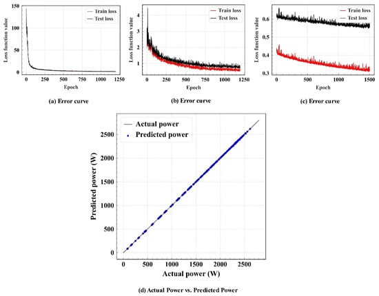
Figure 7.
Model evaluation.
Figure 7d shows the error between the power predicted by the CNN model and the actual power in the test set after the CNN training of the model was completed. It shows that the error between the power predicted by the CNN model and the actual power is low, indicating high fitting accuracy.
4.3. Model Results Discussion
This section presents discussions of the parameters, prediction results, and the applicability of models. Figure 6a–k show the tuning parameter process for ML and EL. The effects of the tuning process correspond to Tables S2 and S3 (in Supplementary Material). Figure 7a–c show the CNN-based parameter-tuning process. The final optimal parameters of all algorithms are presented in Tables S4–S6. From the model evaluation index in Section 2.3, the smaller the values of MSE, RMSE, RAE, MAE, and MAPE, and the closer the value of R2 to one, the better the performance of the model.
- (1)
- ML-based model discussion
Ridge uses L2 regularization and Lasso uses L1 regularization to mitigate overfitting. Elastic Net is a weighted average of Ridge and Lasso regression. LR, Ridge, and Lasso are essentially linear regression methods and are only applicable to linear relationships between data. This study used nonlinear data, so these algorithms were not effective in separating signals from noise and had low prediction precision for the data; therefore, they were not suitable for modeling.
SVR does not overfit on high-dimensional datasets and is suitable for the case of the multiple characteristic variables in this study. It is suitable for small datasets and not for large datasets. Owing to more noise in the dataset in this study, SVR did not perform well in this case. Moreover, it is not easy to update the model when new data are added. Therefore, it was not suitable for modeling in this study.
KNN is computationally intensive, performs well on small datasets, and is not suitable for large datasets. It was not suitable for handling the high-dimensional data in this study. Moreover, the amount of data in this study was quite large, and KNN was not ideal for separating signals from noise.
DT is fast in training and predicting, good at obtaining nonlinear relationships, and also good at handling abnormal samples in our dataset. It is not suitable for small datasets, and when new data are added, it is not easy to update the model, which may be overfitted. DT could not separate signals from noise in this study, and the prediction accuracy was average.
- (2)
- EL-based model discussion
The structure of AdaBoost is simple, and we used the DT model to construct a weak learner. It is fast to train, has higher accuracy, and is not prone to overfitting. It is sensitive to abnormal samples. In this study, there were abnormal samples, which may be given higher weights in the iterations and affect the prediction accuracy of the final strong learner.
RF is the integration of multiple DT trees. The model is random, noise-resistant, and fast to train in parallel. There were 10 features in this study, and the features that took more value divisions tended to have a significant impact on the decisions of RF. There was a relatively noisy dataset; RF cannot correctly handle data samples that are extremely difficult, and its performance was average.
GBR is computationally fast in the prediction phase and can be computed in parallel from tree to tree. We used DT as a weak learner to make GBR more robust and automatically discover higher-order relationships between features. This model uses a robust Huber loss function, which is robust to outliers, and GBR generalizes relatively well to the densely distributed dataset. Owing to the dependency between the weak learner of GBR, it is difficult to train data in parallel, and the model does not perform as well as neural networks on high-dimensional sparse datasets (when handling numerical features).
XGB is an improved algorithm based on GBR. Improvements are made in the following three aspects: optimization of the algorithm, optimization of the algorithm operation efficiency, and optimization of the algorithm robustness. Clearly, from Table 9 and Table S5, XGB outperformed GBR, and it is the best algorithm for the prediction in EL.
- (3)
- DL-based model discussion
The greater the number of layers and parameters in the neural network, the longer the training time. FFN is a fully connected neural network with more weight parameters. Compared with FFN, the sparse connection and weight-sharing strategy of the CNN network can reduce the complexity of the model and make the training and prediction speed fast. The final prediction accuracy was 0.96, and the correlation coefficient was 0.999999, which are both higher than those obtained by FFN, and the prediction accuracy is the highest among all algorithms.
- (4)
- Performance comparison with previous methods
Table 11 shows a performance comparison of the algorithm in this paper with state-of-the-art methods. There has been less literature related to the prediction of PEMFC power using DL-based methods in recent years, and Table 11 compares the use of DL-based methods to predict PEMFC power with the method developed in this study.

Table 11.
Performance comparison with previous methods.
In terms of the source of the data, there was a lack of actual data on PEMFC in most of the literature, as most of the data were obtained using methods based on 3D modeling. This study applied the measured data from the PEMFC system test bench (3 kW) in the laboratory, which included 20 PEMFC characteristic variables, such as cell temperature, hydrogen and air flow, and hydrogen and air backpressure, to demonstrate the model’s reliability and applicability in real-world scenarios.
According to the comparison of algorithms, in most of the literature, only two or three algorithms were compared for the determination of the optimal model for PEMFC power prediction, and the conclusions were not comprehensive enough. Given these circumstances, this paper complements previous work by comparing and optimizing more than ten mainstream conventional ML, EL, and DL methods to propose an optimal model for PEMFC power prediction, providing a strong basis for the selection and optimization of the model.
Comparing the optimization of algorithms, most of the literature did not use techniques to prevent overfitting. In this study, a dropout layer was used to prevent overfitting. This study used the Nadam optimization algorithm. As mentioned in the Optimization Model section, Nadam is an improvement based on Adam. Stronger constraints on the learning rate can improve the performance of the optimization algorithm.
Most of the literature used the MSE loss function. This work used the Huber loss function. From the Structure of the Prediction Model section, it can be seen that Huber is very robust to abnormal samples and solves the problem of MSE’s sensitivity to abnormal samples. In this work, the Swish activation function was chosen. As can be seen from the Optimization Model section, the Swish function solves the drawback that the negative gradient of the ReLU function is 0. Most of the literature used the Tanh or Sigmoid activation function, which lead to premature gradient disappearance in regions with large values, resulting in the slow convergence of the model. The Swish function solves these drawbacks.
The CNN-based model in this paper has an R2 of 0.9999 and a MAPE of 0.0004, which makes it the best-performing model in the current literature.
4.4. I–V Polarization Curves
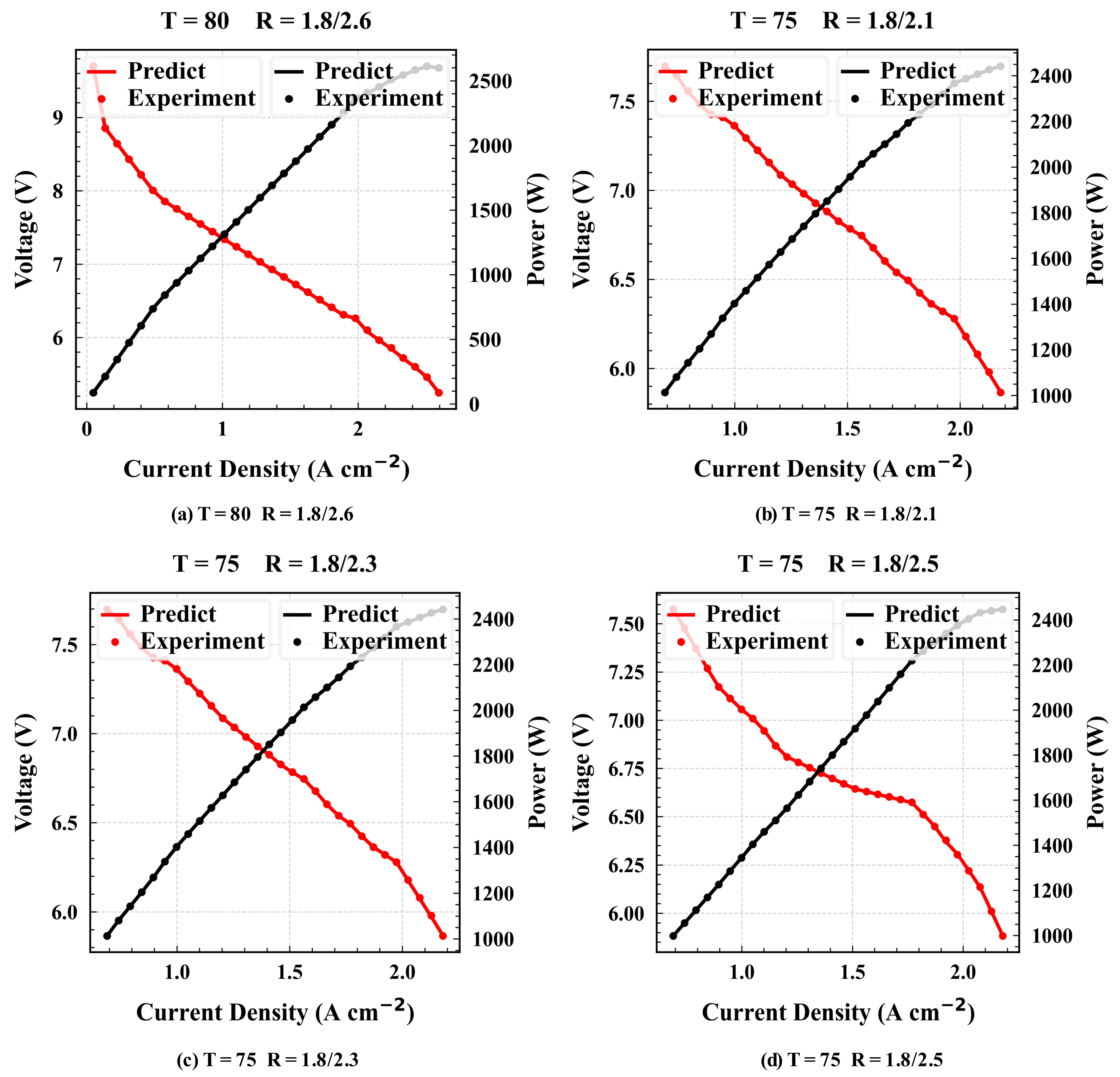
To further demonstrate the authenticity of the CNN-based model, the I–V polarization curves of the measured data from the PEMFC system test bench were fitted with the curves predicted by the model. The polarization curves can represent the performance of the PEMFC, including power. As mentioned in the Feature Selection section (2), the cell temperature (V8) and stoichiometric ratio are important features affecting PEMFC power. Therefore, the polarization curves of PEMFC were predicted with the CNN model based on different cell temperatures and stoichiometric ratios. The polarization curves of the cell temperatures T = 70–T = 80 are shown in Figure 8, where “Predict” represents the results predicted by the model. “Experiment” denotes the actual power, T = 80 denotes the polarization curves of the cell at a temperature of 75 to 80 °C, and R is the stoichiometric ratio (hydrogen stoichiometric ratio (V1)/air stoichiometric ratio (V2)). Similarly, T = 75 represents the data when the cell temperature is between 70 and 75 °C. It is observed in the figure that the predicted results of the model exhibit a satisfactory fitting ability with the actual polarization curves, and the prediction accuracy is high, indicating that the model can predict PEMFC power in the real world. The remaining polarization curves are shown in Figure S3.
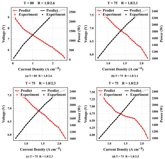
Figure 8.
Polarization curves.
5. Conclusions
This study shifted from traditional CFD-based PEMFC power prediction methods to the development of DL-based methods to efficiently and accurately predict the power of PEMFCs in real-world scenarios. It proposed a prediction method based on Ridge and CNN. The Ridge regression algorithm was used to eliminate abnormal samples of stack power. By comparing mainstream, traditional ML, EL, and DL algorithms, this study designed an optimal model based on CNN to predict PEMFC power in real scenarios, achieving high accuracy and fast prediction speed. Moreover, BN and dropout techniques were adopted to enhance the generalization capability of the model, and the model was optimized with the Swish activation function, Huber function, and Nadam optimization algorithm. The performance of the CNN-based prediction model was verified on actual datasets. The experimental results demonstrate that the I–V polarization curves predicted by the model fit well with the actual I–V polarization curves, and its prediction accuracy was 0.96, which is higher than those of other algorithms.
Compared with traditional CFD-based prediction methods, which consume a lot of time, the CNN-based prediction model can predict PEMFC power within a mere 1 μs, and the iteration speed when training the model is less than 1 s per cycle to reduce the time cost. Trained with real data samples, the model is more suitable than other methods for PEMFC power prediction in real scenarios. These results have proven that the CNN-based model accurately and efficiently predicts the PEMFC power, which can help improve prediction accuracy and speed, and may facilitate further applications of DL-based methods in PEMFC systems.
In this study, the instantaneous power values and performance represented by the polarization curves of the phenomenon at any point in time and in any spatial state can be predicted with high speed and accuracy. This research helps designers to reduce time and cost by iteratively optimizing the PEMFC design solution. The obtained power can also be used for fuel cell parameter tuning, and the fuel cell parameters can be tuned within the desired range. This study contributes to solving the problem of the difficulty in predicting the instantaneous energy consumption of the fuel cell and power cell side of the PEMFC, and it can provide a useful reference for the engineering application of PEMFC power parameter prediction.
After the ideal power is obtained through the predictions of the model, the best combination of characteristics for the maximum power of the fuel cell can also be obtained using a meta-heuristic algorithm. The evaluation of hydrogen-fuel-cell-driven vehicles, also energy-consuming vehicles, such as a comparison of their cost, is significantly influenced by energy consumption data; that is, the level of energy consumption directly affects the operating cost of the tool. This model can be applied to hydrogen fuel cell vehicles in the future with instrument storage to achieve the function of an intelligent power consumption display, providing customers with real-time vehicle power consumption reminders and increasing the power perception dimension of customers. Similarly, it can be applied to predict the instantaneous hydrogen consumption of vehicles. This model applied the data of 10 single cells to predict their power. Migration learning can be applied later to extend the model to predict the PEMFC power of N (N = 5, 20, 25…) single cells or other important characteristic variables, such as the cell temperature and current. In the future, it will be possible to Perform a techno-economic analysis of the hydrogen fuel cell system by the techno-economic analysis method proposed by Roushan Kumar et al [60], i.e., propose a minimum cost prediction based on data processing and analysis. The economic cost of the fuel cell system is reduced and the system efficiency is improved by neural network optimization.
Supplementary Materials
The following supporting information can be downloaded at: https://www.mdpi.com/article/10.3390/su151411010/s1, Figure S1: KDE distribution map; Figure S2: Yeo-Johnson transformation; Figure S3: Polarization curves; Table S1: VIF; Table S2: Prediction results; Table S3: Prediction results; Table S4: Main parameters of the ML model; Table S5: Main parameters of the EL model; Table S6: Main parameters of the DL model.
Author Contributions
Formal analysis, X.L.; writing—original draft preparation, J.Y.; writing—review and editing, Y.W. All authors have read and agreed to the published version of the manuscript.
Funding
This research was funded by the Science and Technology Project of Fujian Province, grant number 2022H0004.
Institutional Review Board Statement
Not applicable.
Informed Consent Statement
Not applicable.
Data Availability Statement
The data presented in this study are available on request from the corresponding author. The data are not publicly available due to the sensitive nature of the questions asked in this study, survey respondents were assured raw data would remain confidential and would not be shared.
Acknowledgments
This work was supported by the Science and Technology Project of Fujian Province (No. 2022H0004). The authors thank the Jia Geng Laboratory of Xiamen University for providing the actual measurement data for the PEMFC experiment in this study.
Conflicts of Interest
The authors declare no conflict of interest.
Nomenclature
| V0 | Current (A) | CFD | Computational fluid dynamics |
| V1 | Hydrogen stoichiometric ratio | 3D | Three-dimensional |
| V2 | Air stoichiometric ratio | 2D | Two-dimensional |
| V3 | Hydrogen backpressure (MPa) | Eq | Equation |
| V4 | Air backpressure (MPa) | AI | Artificial intelligence |
| V5 | Hydrogen inlet pressure (MPa) | ML | Machine learning |
| V6 | Air inlet pressure (MPa) | EL | Ensemble learning |
| V7 | Circulating water inlet temperature (°C) | DL | Deep learning |
| V8 | Circulating water outlet temperature (°C) | MSE | Mean Square Error |
| V9 | Circulating water conductivity (us cm−1) | MAPE | Mean Absolute Percentage Error |
| V10 | Hydrogen inlet temperature (°C) | R2 | Determination Coefficient |
| V11 | Air inlet temperature (°C) | RMSE | Root Mean Square Error |
| V12 | Hydrogen humidification tank temperature (°C) | RAE | Relative Absolute Error |
| V13 | Air humidification tank temperature (°C) | RF | Random Forest |
| V14 | Hydrogen inlet insulation temperature (°C) | GBR | Gradient Boosting Regression |
| V15 | Air inlet insulation temperature (°C) | XGB | Extreme Gradient Boosting |
| V16 | Hydrogen inlet dew point (°C) | CNN | Convolutional neural network |
| V17 | Air inlet dew point (°C) | FFN | Feedforward neural network |
| V18 | Hydrogen flow rate (L min−1) | AdaBoost | AdaBoost regressor |
| V19 | Air flow rate (L min−1) | LR | Linear regression |
| Target | Power (W cm−2) | DT | Decision Tree |
| PEMFC | Proton exchange membrane fuel cell | KNN | K-Nearest Neighbor Regression |
| PEM | Proton exchange membrane | Elastic Net | Elastic Net Regression |
| GDL | Gas diffusion layer | SVR | Support Vector Regression |
| BP | Bipolar plate | Lasso | Lasso regression |
| CL | Catalyst layer | Ridge | Ridge regression |
| MPL | Microporous Layer | BN | Batch normalization |
| MEA | Membrane electrode assembly | Nadam | Nesterov-accelerated adaptive moment estimation |
References
- Benmouna, A.; Becherif, M.; Depernet, D.; Gustin, F.; Ramadan, H.S.; Fukuhara, S. Fault diagnosis methods for Proton Exchange Membrane Fuel Cell system. Int. J. Hydrogen Energy 2017, 42, 1534–1543. [Google Scholar] [CrossRef]
- Barreto, L.; Makihira, A.; Riahi, K. The hydrogen economy in the 21st century: A sustainable development scenario. Int. J. Hydrogen Energy 2003, 28, 267–284. [Google Scholar] [CrossRef]
- Dincer, I. Technical, environmental and exergetic aspects of hydrogen energy systems. Int. J. Hydrogen Energy 2002, 27, 265–285. [Google Scholar] [CrossRef]
- Song, W.J.; Chen, H.; Guo, H.; Ye, F.; Li, J.R. Research progress of proton exchange membrane fuel cells utilizing in high altitude environments. Int. J. Hydrogen Energy 2022, 47, 24945–24962. [Google Scholar] [CrossRef]
- Camacho, M.D.L.N.; Jurburg, D.; Tanco, M. Hydrogen fuel cell heavy-duty trucks: Review of main research topics. Int. J. Hydrogen Energy 2022, 47, 29505–29525. [Google Scholar] [CrossRef]
- Chang, K.Y. The optimal design for PEMFC modeling based on Taguchi method and genetic algorithm neural networks. Int. J. Hydrogen Energy 2011, 36, 13683–13694. [Google Scholar] [CrossRef]
- Gabbasa, M.; Sopian, K.; Fudholi, A.; Asim, N. A review of unitized regenerative fuel cell stack: Material, design and research achievements. Int. J. Hydrogen Energy 2014, 39, 17765–17778. [Google Scholar] [CrossRef]
- Li, H.; Xu, B.; Du, C.; Yang, Y. Performance prediction and power density maximization of a proton exchange membrane fuel cell based on deep belief network. J. Power Sources 2020, 461, 228154. [Google Scholar] [CrossRef]
- Hu, B.; Chang, F.L.; Xiang, L.Y.; He, G.J.; Cao, X.W.; Yin, X.C. High performance polyvinylidene fluoride/graphite/multi-walled carbon nanotubes composite bipolar plate for PEMFC with segregated conductive networks. Int. J. Hydrogen Energy 2021, 46, 25666–25676. [Google Scholar] [CrossRef]
- Jyotheeswara Reddy, K.; Natarajan, S. Energy sources and multi-input DC-DC converters used in hybrid electric vehicle applications—A review. Int. J. Hydrogen Energy 2018, 43, 17387–17408. [Google Scholar] [CrossRef]
- Mehrpooya, M.; Ghorbani, B.; Jafari, B.; Aghbashlo, M.; Pouriman, M. Modeling of a single cell micro proton exchange membrane fuel cell by a new hybrid neural network method. Therm. Sci. Eng. Prog. 2018, 7, 8–19. [Google Scholar] [CrossRef]
- Han, I.S.; Chung, C.B. Performance prediction and analysis of a PEM fuel cell operating on pure oxygen using data-driven models: A comparison of artificial neural network and support vector machine. Int. J. Hydrogen Energy 2016, 41, 10202–10211. [Google Scholar] [CrossRef]
- Kheirandish, A.; Motlagh, F.; Shafiabady, N. ScienceDirect Dynamic modelling of PEM fuel cell of power electric bicycle system. Int. J. Hydrogen Energy 2016, 41, 9585–9594. [Google Scholar] [CrossRef]
- Kheirandish, A.; Shafiabady, N.; Dahari, M. ScienceDirect Modeling of commercial proton exchange membrane fuel cell using support vector machine. Int. J. Hydrogen Energy 2016, 41, 11351–11358. [Google Scholar] [CrossRef]
- Wang, Y.; Seo, B.; Wang, B.; Zamel, N.; Jiao, K.; Adroher, X.C. Fundamentals, materials, and machine learning of polymer electrolyte membrane fuel cell technology. Energy AI 2020, 1, 100014. [Google Scholar] [CrossRef]
- Song, G.-H.; Meng, H. Numerical modeling and simulation of PEM fuel cells: Progress and perspective. Acta Mech. Sin. 2013, 29, 318–334. [Google Scholar] [CrossRef]
- Demuren, A.; Edwards, R.L. Modeling Proton Exchange Membrane Fuel Cells—A Review. In 50 Years of CFD in Engineering Sciences; Runchal, A., Ed.; Springer: Singapore, 2020. [Google Scholar] [CrossRef]
- Macauley, N.; Lujan, R.W.; Spernjak, D.; Hussey, D.S.; Jacobson, D.L.; More, K.; Borup, R.L.; Mukundan, R. Durability of Polymer Electrolyte Membrane Fuel Cells Operated at Subfreezing Temperatures. J. Electrochem. Soc. 2016, 163, F1317–F1329. [Google Scholar] [CrossRef]
- Wu, H.W. A review of recent development: Transport and performance modeling of PEM fuel cells. Appl. Energy 2016, 165, 81–106. [Google Scholar] [CrossRef]
- Zheng, L.; Hou, Y.; Zhang, T.; Pan, X. Performance prediction of fuel cells using long short-term memory recurrent neural network. Int. J. Energy Res. 2021, 45, 9141–9161. [Google Scholar] [CrossRef]
- Lu, L.; Ouyang, M.; Huang, H.; Pei, P.; Yang, F. A semi-empirical voltage degradation model for a low-pressure proton exchange membrane fuel cell stack under bus city driving cycles. J. Power Sources 2007, 164, 306–314. [Google Scholar] [CrossRef]
- Moreira, M.V.; da Silva, G.E. A practical model for evaluating the performance of proton exchange membrane fuel cells. Renew. Energy 2009, 34, 1734–1741. [Google Scholar] [CrossRef]
- Hu, Z. A reconstructed fuel cell life-prediction model for a fuel cell hybrid city bus. Energy Convers. Manag. 2018, 156, 723–732. [Google Scholar] [CrossRef]
- Saleem, S.; Hussain, K. Membrane-hydration-state detection in proton exchange membrane fuel cells using improved ambient-condition-based dynamic model. Int. J. Energy Res. 2020, 44, 869–889. [Google Scholar] [CrossRef]
- Fraser, S.D.; Hacker, V. An empirical fuel cell polarization curve fitting equation for small current densities and no-load operation. J. Appl. Electrochem. 2008, 38, 451–456. [Google Scholar] [CrossRef]
- Ou, M.; Zhang, R.; Shao, Z.; Li, B.; Yang, D.; Ming, P.; Zhang, C. A novel approach based on semi-empirical model for degradation prediction of fuel cells. J. Power Sources 2021, 488, 229435. [Google Scholar] [CrossRef]
- Huo, W.; Li, W.; Zhang, Z.; Sun, C.; Zhou, F.; Gong, G. Performance prediction of proton-exchange membrane fuel cell based on convolutional neural network and random forest feature selection. Energy Convers. Manag. 2021, 243, 114367. [Google Scholar] [CrossRef]
- Sun, P.; Zhou, S.; Hu, Q.; Liang, G. Numerical Study of a 3D Two-Phase PEM Fuel Cell Model Via a Novel Automated Finite Element/Finite Volume Program Generator. Commun. Comput. Phys. 2012, 11, 65–98. [Google Scholar] [CrossRef]
- Zhang, J.; Zhang, C.; Hao, D.; Ni, M.; Huang, S.; Liu, D.; Zheng, Y. 3D non-isothermal dynamic simulation of high temperature proton exchange membrane fuel cell in the start-up process. Int. J. Hydrogen Energy 2021, 46, 2577–2593. [Google Scholar] [CrossRef]
- Xie, B.; Zhang, G.; Xuan, J.; Jiao, K. Three-dimensional multi-phase model of PEM fuel cell coupled with improved agglomerate sub-model of catalyst layer. Energy Convers. Manag. 2019, 199, 112051. [Google Scholar] [CrossRef]
- Chávez-Ramírez, A.U.; Muñoz-Guerrero, R.; Durón-Torres, S.M.; Ferraro, M.; Brunaccini, G.; Sergi, F.; Antonucci, V.; Arriaga, L.G. High power fuel cell simulator based on artificial neural network. Int. J. Hydrogen Energy 2010, 35, 12125–12133. [Google Scholar] [CrossRef]
- Fadzillah, D.M.; Rosli, M.I.; Talib, M.Z.M.; Kamarudin, S.K.; Daud, W.R.W. Review on microstructure modelling of a gas diffusion layer for proton exchange membrane fuel cells. Renew. Sustain. Energy Rev. 2017, 77, 1001–1009. [Google Scholar] [CrossRef]
- Niu, Z.; Wang, Y.; Luo, K.; Li, H.; Wang, Y. Two-Phase Flow Dynamics in the Gas Diffusion Layer of Proton Exchange Membrane Fuel Cells: Volume of Fluid Modeling and Comparison with Experiment. J. Electrochem. Soc. 2018, 165, 613–620. [Google Scholar] [CrossRef]
- Benner, J.; Mortazavi, M.; Santamaria, A.D. Numerical Simulation of Droplet Emergence and Growth From Gas Diffusion Layers (GDLs) in Proton Exchange Membrane (PEM) Fuel Cell Flow Channels. In Proceedings of the ASME 2018 International Mechanical Engineering Congress and Exposition, Pittsburgh, PA, USA, 9–15 November 2018. [Google Scholar] [CrossRef]
- Wang, Y.; Wang, C.Y. Ultra large-scale simulation of polymer electrolyte fuel cells. J. Power Sources 2006, 153, 130–135. [Google Scholar] [CrossRef]
- Zhang, G.; Bao, Z.; Xie, B.; Wang, Y.; Jiao, K. Three-dimensional multi-phase simulation of PEM fuel cell considering the full morphology of metal foam flow field. Int. J. Hydrogen Energy 2021, 46, 2978–2989. [Google Scholar] [CrossRef]
- Tian, P.; Liu, X.; Luo, K.; Li, H.; Wang, Y. Deep learning from three-dimensional multiphysics simulation in operational optimization and control of polymer electrolyte membrane fuel cell for maximum power. Appl. Energy 2021, 288, 116632. [Google Scholar] [CrossRef]
- Bao, Z.; Wang, Y.; Jiao, K. Liquid droplet detachment and dispersion in metal foam flow field of polymer electrolyte membrane fuel cell. J. Power Sources 2020, 480, 229150. [Google Scholar] [CrossRef]
- Zhang, G.; Yuan, H.; Wang, Y.; Jiao, K. Three-dimensional simulation of a new cooling strategy for proton exchange membrane fuel cell stack using a non-isothermal multiphase model. Appl. Energy 2019, 255, 113865. [Google Scholar] [CrossRef]
- Wang, B.; Xie, B.; Xuan, J.; Jiao, K. AI-based optimization of PEM fuel cell catalyst layers for maximum power density via data-driven surrogate modeling. Energy Convers. Manag. 2020, 205, 112460. [Google Scholar] [CrossRef]
- Wang, F.K.; Mamo, T.; Cheng, X.B. Bi-directional long short-term memory recurrent neural network with attention for stack voltage degradation from proton exchange membrane fuel cells. J. Power Sources 2020, 461, 228170. [Google Scholar] [CrossRef]
- Khajeh-Hosseini-Dalasm, N.; Ahadian, S.; Fushinobu, K.; Okazaki, K.; Kawazoe, Y. Prediction and analysis of the cathode catalyst layer performance of proton exchange membrane fuel cells using artificial neural network and statistical methods. J. Power Sources 2011, 196, 3750–3756. [Google Scholar] [CrossRef]
- Zhang, G.; Wu, L.; Jiao, K.; Tian, P.; Wang, B.; Wang, Y.; Liu, Z. Optimization of porous media flow field for proton exchange membrane fuel cell using a data-driven surrogate model. Energy Convers. Manag. 2020, 226, 113513. [Google Scholar] [CrossRef]
- Park, J.Y.; Lee, Y.H.; Lim, I.S.; Kim, Y.S.; Kim, M.S. Prediction of local current distribution in polymer electrolyte membrane fuel cell with artificial neural network. Int. J. Hydrogen Energy 2021, 46, 20678–20692. [Google Scholar] [CrossRef]
- Özçelep, Y.; Sevgen, S.; Samli, R. A study on the hydrogen consumption calculation of proton exchange membrane fuel cells for linearly increasing loads: Artificial Neural Networks vs Multiple Linear Regression. Renew. Energy 2020, 156, 570–578. [Google Scholar] [CrossRef]
- Hua, Z.; Zheng, Z.; Péra, M.C.; Gao, F. Remaining useful life prediction of PEMFC systems based on the multi-input echo state network. Appl. Energy 2020, 265, 114791. [Google Scholar] [CrossRef]
- Chen, K.; Laghrouche, S.; Djerdir, A. Degradation prediction of proton exchange membrane fuel cell based on grey neural network model and particle swarm optimization. Energy Convers. Manag. 2019, 195, 810–818. [Google Scholar] [CrossRef]
- Saengrung, A.; Abtahi, A.; Zilouchian, A. Neural network model for a commercial PEM fuel cell system. J. Power Sources 2007, 172, 749–759. [Google Scholar] [CrossRef]
- Javed, K.; Gouriveau, R.; Zerhouni, N.; Hissel, D. Prognostics of Proton Exchange Membrane Fuel Cells stack using an ensemble of constraints based connectionist networks. J. Power Sources 2016, 324, 745–757. [Google Scholar] [CrossRef]
- Hua, Z. Lifespan Prediction of Proton Exchange Membrane Fuel Cell System. Other. Université Bourgogne Franche-Comté. 2021. Available online: https://theses.hal.science/tel-03793342/document (accessed on 1 July 2022).
- Wilberforce, T.; Olabi, A.G. Proton exchange membrane fuel cell performance prediction using artificial neural network. Int. J. Hydrogen Energy 2021, 46, 6037–6050. [Google Scholar] [CrossRef]
- Nanadegani, F.S.; Lay, E.N.; Iranzo, A.; Salva, J.A.; Sunden, B. On neural network modeling to maximize the power output of PEMFCs. Electrochim. Acta 2020, 348, 136345. [Google Scholar] [CrossRef]
- Li, H.; Xu, B.; Lu, G.; Du, C.; Huang, N. Multi-objective optimization of PEM fuel cell by coupled significant variables recognition, surrogate models and a multi-objective genetic algorithm. Energy Convers. Manag. 2021, 236, 114063. [Google Scholar] [CrossRef]
- Meera, C.S.; Sunny, S.; Singh, R.; Sairam, P.S.; Kumar, R.; Emannuel, J. Automated precise liquid transferring system. In Proceedings of the 2014 IEEE 6th India International Conference on Power Electronics (IICPE), Kurukshetra, India, 8–10 December 2014; pp. 1–6. [Google Scholar] [CrossRef]
- Ding, R.; Zhang, S.; Chen, Y.; Rui, Z.; Hua, K.; Wu, Y.; Li, X.; Duan, X.; Wang, X.; Li, J.; et al. Application of Machine Learning in Optimizing Proton Exchange Membrane Fuel Cells: A Review. Energy AI 2022, 9, 100170. [Google Scholar] [CrossRef]
- Soleimani, S.; Heydari, A.; Fattahi, M. Swelling prediction of calcium alginate/cellulose nanocrystal hydrogels using response surface methodology and artificial neural network. Ind. Crops Prod. 2023, 192, 116094. [Google Scholar] [CrossRef]
- Feng, Z.; Huang, J.; Jin, S.; Wang, G.; Chen, Y. Artificial intelligence-based multi-objective optimisation for proton exchange membrane fuel cell: A literature review. J. Power Sources 2022, 520, 230808. [Google Scholar] [CrossRef]
- Cheddie, D.; Munroe, N. Review and comparison of approaches to proton exchange membrane fuel cell modeling. J. Power Sources 2005, 147, 72–84. [Google Scholar] [CrossRef]
- Wang, J.; Li, S.; An, Z.; Jiang, X.; Qian, W.; Ji, S. Batch-normalized deep neural networks for achieving fast intelligent fault diagnosis of machines. Neurocomputing 2019, 329, 53–65. [Google Scholar] [CrossRef]
- Kumar, R.; Kumar, A.; Gupta, M.K.; Yadav, J.; Jain, A. Solar tree-based water pumping for assured irrigation in sustainable Indian agriculture environment. Sustain. Prod. Consum. 2022, 33, 15–27. [Google Scholar] [CrossRef]
Disclaimer/Publisher’s Note: The statements, opinions and data contained in all publications are solely those of the individual author(s) and contributor(s) and not of MDPI and/or the editor(s). MDPI and/or the editor(s) disclaim responsibility for any injury to people or property resulting from any ideas, methods, instructions or products referred to in the content. |
© 2023 by the authors. Licensee MDPI, Basel, Switzerland. This article is an open access article distributed under the terms and conditions of the Creative Commons Attribution (CC BY) license (https://creativecommons.org/licenses/by/4.0/).

