A New Combined Prediction Model for Ultra-Short-Term Wind Power Based on Variational Mode Decomposition and Gradient Boosting Regression Tree

Abstract

Wind power is an essential component of renewable energy. It enables the conservation of conventional energy sources such as coal and oil while reducing greenhouse gas emissions. To address the stochastic and intermittent nature of ultra-short-term wind power, a combined prediction model based on variational mode decomposition (VMD) and gradient boosting regression tree (GBRT) is proposed. Firstly, VMD is utilized to decompose the original wind power signal into three meaningful components: the long-term component, the short-term component, and the randomness component. Secondly, based on the characteristics of these three components, a support vector machine (SVM) is selected to predict the long-term and short-term components, while gated recurrent unit-long short-term memory (GRU-LSTM) is employed to predict the randomness component. Particle swarm optimization (PSO) is utilized to optimize the structural parameters of the SVM and GRU-LSTM combination for enhanced prediction accuracy. Additionally, a GBRT model is employed to predict the residuals. Finally, the rolling predicted values of the three components and residuals are aggregated. A deep learning framework using TensorFlow 2.0 has been built on the Python platform, and a dataset measured from a wind farm has been utilized for learning and prediction. The comparative analysis reveals that the proposed model exhibits superior short-term wind power prediction performance, with a mean squared error, mean absolute error, and coefficient of determination of 0.0244, 0.1185, and 0.9821, respectively.

1. Introduction

With the introduction of the dual carbon goals in the new power system, the proportion of renewable energy such as wind power in electricity supplies has been increasing year by year [1]. Due to inherent characteristics such as volatility, randomness, and non-linearity, wind power generation is difficult to predict [2]. Additionally, wind energy is characterized by its fluctuating and intermittent nature [3], which is unfavorable for the safe [4] and stable operation [5] and economic dispatch [6] of the power system. Improving the accuracy of ultra-short-term wind power prediction can mitigate the impact of wind power grid integration. Wind power forecasting provides important guidance for grid operations [7].

Currently, wind power forecasting methods primarily utilize artificial intelligence algorithms, which learn models based on historical data such as wind direction, wind speed, and power. Wind power prediction using intelligent algorithms can be further categorized into single-algorithm prediction methods and combination prediction methods employing multiple algorithms. Single prediction methods include grey prediction [8], locally recurrent neural networks [9], support vector machines [10], and others. Due to the limitations of single algorithms, the accuracy of single prediction methods is often poor. To improve the prediction accuracy, it is common to compensate for the deficiencies of a single algorithm by employing other algorithms, which can further enhance the prediction accuracy. In reference [11], for short-term wind power prediction in wind farms, a prediction model was constructed using Bayesian dynamic clustering (BCD) and support vector regression (SVR). In reference [12], to further improve the prediction accuracy of the least squares support vector machine for wind power, an autoregressive integrated moving average model (ARIMA) was used to model the linear component of wind power. In reference [13], improved simplified swarm optimization was employed to optimize the parameters of the multi-layer perceptron (MLP) artificial neural network model. In reference [14], the convolutional neural network (CNN) was first used to extract multiple features from wind power and its influencing factors, and then these features were input into the long and short-term memory (LSTM) network for prediction, ultimately achieving time series forecasting of wind power. In reference [15], a new technique for investigating wind power prediction error in the multi-objective domain has been proposed. It presented an enhanced multi-objective exchange market algorithm (EMEMA) for solving multi-objective problems. The simulation results demonstrated the algorithm’s superior performance.

To further enhance their ability to extract temporal information and improve their resistance to interference and generalization, combined algorithms of machine learning and load decomposition are often employed [16,17]. In order to fully utilize the effective information in historical data and further improve the prediction accuracy of wind power generation, reference [18] proposed an ensemble empirical mode decomposition (EMD) and LSTM neural network. Reference [19] combined EMD with deep long-term memory (DLSTM) to construct the EMD-DLSTM prediction model. Due to the mode mixing and over-decomposition issues in EMD, Dragomiretskiy et al. [20] proposed a novel signal decomposition method called variational mode decomposition (VMD) based on Fourier decomposition to effectively address these problems. VMD utilizes Wiener filtering for denoising and exhibits excellent noise robustness. It can variably and non-recursively extract a specified number of modal components from non-stationary and non-linear time series signals. It is an adaptive signal decomposition method, and each analytical signal has a physical meaning. By using VMD, historical wind power can be decomposed into several components with different central frequencies, which can then be combined with selected meteorological features. VMD can effectively avoid mode mixing and the endpoint effects generated by EMD. However, the convergence and anti-interference properties of its intrinsic mode components are dependent on the choice of penalty coefficients. In reference [21], a new hybrid model based on VMD and LSTM was proposed, which has the functions of eliminating seasonal factors and error correction. The experimental results demonstrate that the prediction accuracy of this model is significantly higher than that of the comparative models. In reference [22], VMD was utilized to decompose the data, resulting in wind speed subsequences with different frequencies but strong regularity. Based on this, a radial basis function neural network was used to model and predict each subsequence. The important references are summarized in

Table 1. Summary of references.

Literature	Methods	Application
[11]	BCD, SVR	Forecasting wind generation
[12]	ARFIMA, LSSVM	Wind power prediction
[13]	ISSO, MLP	Forecasting wind power
[14]	CNN, LSTM	Wind power prediction
[15]	EMEMA	Wind power prediction error in the multi-objective environmental economics problem
[16]	VMD, SG, LSTM	Short-term power load prediction
[17]	VMD, NN	Wind speed prediction
[18]	EMD, LSTM	Short-term wind power prediction
[19]	EMD, DLSTM	Ultra-short-term prediction of wind power
[21]	VMD, LSTM	Load forecasting
[22]	VMD, RBF	Wind power prediction

.

Ultra-short-term power sequences are characterized by the complexity and difficulty in accurate prediction due to the influence of multiple external factors. Therefore, in this paper, a new combined model is proposed for ultra-short-term wind power prediction based on VMD and gradient boosting regression tree (GBRT). The model takes advantage of SVM for high predictive performance on long- and short-term components, as well as the strong predictive performance of GRU-LSTM for random components. To enhance the optimization efficiency of SVM and GRU-LSTM, a PSO algorithm is also combined so that their optimization efficiency and convergence speed can be improved. On this basis, GBRT is employed to predict the overall residuals, further enhancing the prediction accuracy of the model. The high prediction accuracy is beneficial to reduce the impact of the wind power grid connection and improve the stability of the power operation, and to provide the basis for the dispatching operation of the power grid dispatching department.

The organization of the paper is as follows. In Section 2, the overall framework of the prediction model is presented, and the VMD model, PSO combined with SVM model, PSO combined with GRU and LSTM model, and the GBRT model are established separately. In Section 3, the models are trained and tested using an actual wind power generation dataset. The prediction results are analyzed using the mean squared error (MSE), mean absolute error (MAE), and the coefficient of determination R², demonstrating the effectiveness of the proposed model. Section 4 provides a brief summary.

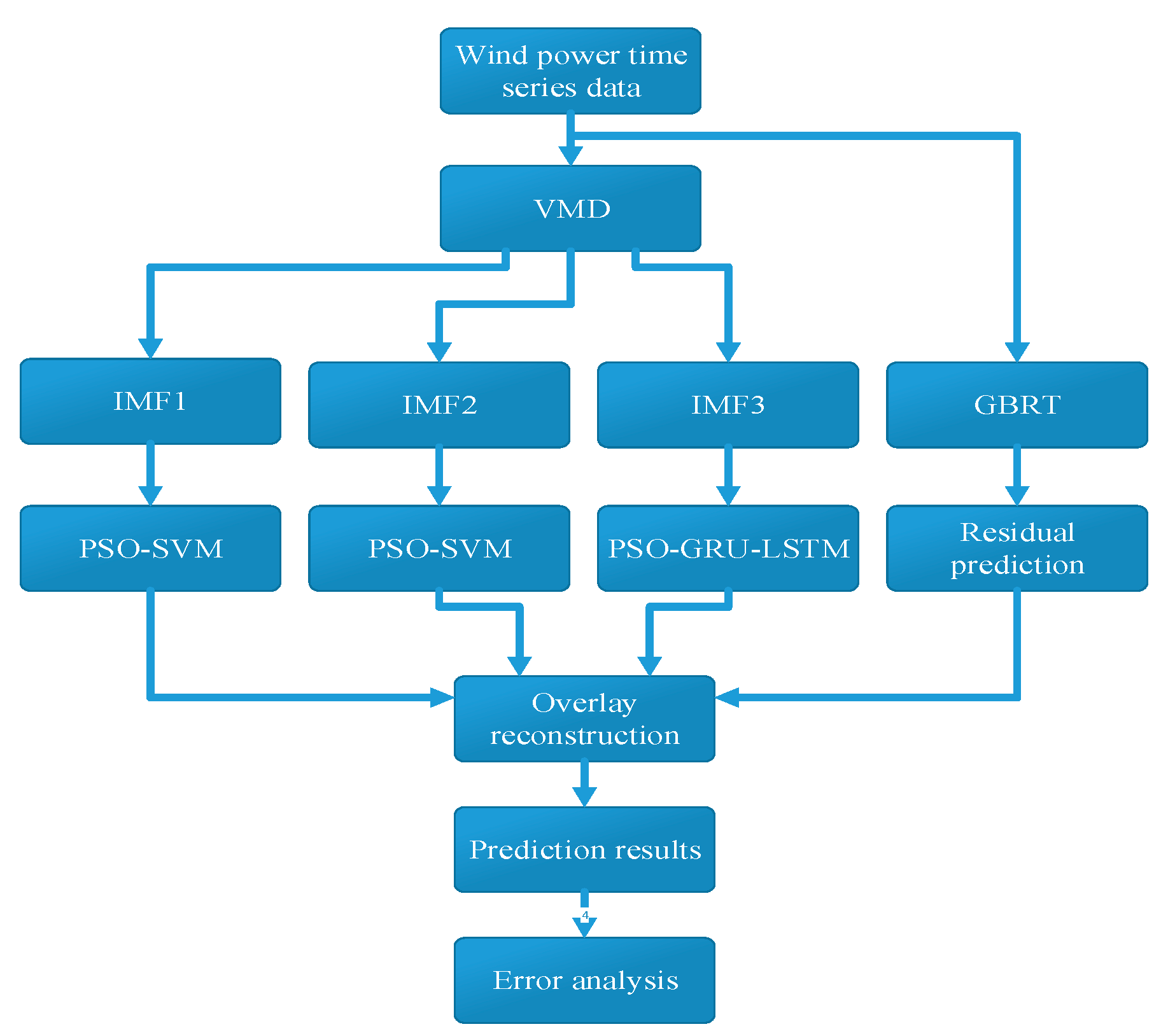
2. Overall Framework of the Prediction Model

The wind power prediction model framework is shown in Figure 1, where each module is trained separately to obtain the trained model. The prediction process of the model is as follows: firstly, the wind power time series data are decomposed into three components, IMF1, IMF2, and IMF3, through VMD. Secondly, based on the characteristics of IMF1, IMF2, and IMF3, PSO-SVM is selected to predict the long-term and short-term components (IMF1 and IMF2), while PSO-GRU-LSTM is used to predict the stochastic component (IMF3). Next, the original wind power sequence is inputted into the GBRT for the residual prediction. Finally, the rolling predicted values of the reconstructed four components are combined to obtain the final prediction results, which are then analyzed for errors.

VMD can effectively avoid mode mixing and the endpoint effects generated by EMD. In Figure 1, VMD is used to decompose the original wind power signal into three components that align with the actual characteristics of the power grid data: the long-term component IMF1, the short-term component IMF2, and the randomness component IMF3. This decomposition aims to improve the prediction accuracy by separately forecasting each component. The inclusion of GBRT in the proposed approach is to utilize the boosting method to integrate multiple weak learners into a strong learner and predict the overall residuals, further enhancing the prediction accuracy. Compared to conventional regression tree algorithms, GBRT has advantages such as strong generalization and prediction capabilities. However, it lacks the ability for parallel processing.

2.1. Variational Mode Decomposition

VMD achieves a stable decomposition of signals and extracts hierarchical information by solving a variational problem. VMD essentially decomposes the original signal into several distinct intrinsic mode functions (IMFs), where each function represents a single-component amplitude-modulated and frequency-modulated signal with a different center frequency. By iteratively searching for the optimal solution of the variational mode functions model, the center frequency of each function is determined. The mathematical theory of the variational problem can be represented as [23]:

$$\{\begin{array}{l}\underset{\left\{y_k\right\},\left\{{\omega }_k\right\}}{\min }\left\{{\displaystyle \sum _{k=1}^K{\displaystyle {\Vert {\partial }_t\left[\left(\delta \left(t\right)+\frac{j}{\pi t}\right)\ast y_k\left(t\right)\right]e^{-j{\omega }_{k}t}\Vert }_2^2}}\right\}\hfill \\ \mathrm{s}.\mathrm{t}.{\displaystyle {\sum }_k{y}_k=z\left(t\right)}\hfill \end{array}$$

(1)

where {y_k} = {y₁, …, y_K} and {ω_k} = {ω₁, …, ω_K} represent the sets of all modes and their respective center frequencies.

To transform the constrained variational problem into an unconstrained optimization problem, quadratic penalties α and Lagrange multipliers λ are introduced to enhance reconstruction fidelity and enforce constraints more strictly, as expressed in the following equation.

$$L\left\{\left\{y_k\right\},\left\{{\omega }_k\right\},\lambda \right\}=\alpha \left\{{\displaystyle \sum _{k=1}^K{\displaystyle {\Vert {\partial }_t\left[\left(\delta \left(t\right)+\frac{j}{\pi t}\right)y_k\left(t\right)\right]e^{-j{\omega }_{k}t}\Vert }_2^2}+{\displaystyle {\Vert z\left(t\right)-{\displaystyle \sum _{k=1}^K{y}_k}\Vert }_2^2}\langle \lambda \left(t\right),z\left(t\right)-{\displaystyle \sum _{k=1}^K{y}_k}\left(t\right)\rangle }\right\}$$

(2)

The minimization problem can be solved using an iterative counting optimization method, and the solution to Equation (2) can be obtained using the alternate direction method of multipliers (ADMM) [24,25]. The updates for y_k, ω_k, and λ can be obtained through ADMM as follows:

$${\displaystyle {\widehat{y}}_k^{n+1}}\left(\omega \right)=\frac{\widehat{z}\left(\omega \right)-{\displaystyle {\sum }_{i\ne k}{\widehat{y}}_i\left(\omega \right)+\frac{\widehat{\lambda }\left(\omega \right)}{2}}}{1+2\alpha {\left(\omega -{\omega }_k\right)}^2}$$

(3)

$${\displaystyle {\widehat{\omega }}_k^{n+1}}=\frac{{\displaystyle {\displaystyle {\int }_0^{\infty }}\omega {\left|{\widehat{y}}_k\left(\omega \right)\right|}^{2}d\omega }}{{\displaystyle {\displaystyle {\int }_0^{\infty }}{\left|{\widehat{y}}_k\left(\omega \right)\right|}^{2}d\omega }}$$

(4)

$${\widehat{\lambda }}^{n+1}\left(\omega \right)={\widehat{\lambda }}^n\left(\omega \right)+\tau \left(\widehat{z}\left(\omega \right)-{\displaystyle \sum _k{\displaystyle {\widehat{y}}_k^{n+1}}\left(\omega \right)}\right)$$

(5)

where $\widehat{z}\left(\omega \right)$, ${\widehat{y}}_i\left(\omega \right)$, and $\widehat{\lambda }\left(\omega \right)$ represent the Fourier transforms of each variable, and n is the number of iterations.

In this study, the wind power time series data are decomposed into three components, IMF1, IMF2, and IMF3, using VMD. The decomposition process is as follows:

• Initialize the Lagrange multipliers, sets of modal functions, and instantaneous frequencies as ${\widehat{\lambda }}^1$, $\left\{{\displaystyle {\widehat{y}}_k^1}\right\}$ and $\left\{{\displaystyle {\omega }_k^1}\right\}$, where n = 0.
• Let n = n + 1 and enter the iterative loop.
• Update the y_k, ω_k and λ according to Equations (3)–(5).
• Set a threshold ε and evaluate the condition given by Equation (6). If the computed result is smaller than ε, satisfying the condition in Equation (6), stop the iteration. Otherwise, continue the iteration.

  $${\displaystyle {\sum }_k\frac{{\displaystyle {\Vert {\displaystyle {\widehat{y}}_k^{n+1}}-{\displaystyle {\widehat{y}}_k^n}\Vert }_2^2}}{{\displaystyle {\Vert {\displaystyle {\widehat{y}}_k^n}\Vert }_2^2}}}<\epsilon$$

  (6)

Although VMD has advantages in preventing mode mixing and endpoint effects, it requires a manual determination of the number of modes. If the number of modes is too small, the decomposition features may not be clearly visible, while an excessive number of modes may lead to over-decomposition. Therefore, the choice of the number of modes greatly affects the decomposition results. Currently, the commonly used method for selecting the number of modes is the center frequency method. However, it has limitations in practical applications. When the center frequencies of the decomposed modes are close to each other, it may result in multi-mode decomposition, which affects the decomposition results. To overcome this limitation, in this study, we propose a method to decompose the wind power signal into three components: long-term component IMF1, short-term component IMF2, and stochastic component IMF3.

2.2. PSO Module

The PSO algorithm initializes a swarm of random particles in the D-dimensional search space to track the current best particle and search for the optimal value. By adjusting and experimenting with its parameters iteratively, PSO can partially avoid the issue of being trapped in local optima and instead find the global optimum. The PSO algorithm has gained attention and been widely applied in various fields [26,27] due to its simplicity, ease of implementation, robust performance, fast convergence speed, and reduced tendency to become stuck in local optima.

The core of this algorithm lies in comparing the fitness value of each particle with its individual best and global best values, determining whether to update the individual best value and global best value accordingly. If updates are made to both values, the particle will update its velocity and position based on Equations (7) and (8) [28]:

$${\displaystyle v_{id}^{k+1}}=u{\displaystyle v_{id}^k}+c_1{r}_1\left({\displaystyle p_{id}^k}-{\displaystyle x_{id}^k}\right)+c_2{r}_2\left({\displaystyle p_{gd}^k}-{\displaystyle x_{id}^k}\right)$$

(7)

$${\displaystyle x_{id}^{k+1}}={\displaystyle x_{id}^k}+{\displaystyle v_{id}^{k+1}}$$

(8)

where v_id represents the particle velocity, x_id represents the particle position, d = [1, 2, …, D] denotes the spatial dimension, and i = [1, 2, …, M] represents the population size. c₁ and c₂ are the acceleration factors that enable the particles to have self-awareness and learn from other individuals, typically set to 2. r₁ and r₂ are random numbers between 0 and 1. ${\displaystyle p_{id}^k}$ and ${\displaystyle p_{gd}^k}$ represent the individual and global best values, respectively. u is the inertia weight.

2.3. PSO-SVM Module

SVM exhibits strong adaptability and outstanding learning ability when dealing with small-sample non-linear and other types of data. However, a single SVM may struggle to meet the required prediction accuracy. Therefore, PSO is employed to optimize the kernel function parameter γ and penalty coefficient C, aiming to enhance the prediction accuracy.

The training dataset is as follows:

$$S=\left\{s_i|s_i=\left(x_i,y_i\right)x_i,y_i\in R^n,i=1,2,\cdots ,l\right\}$$

(9)

The optimal classification hyperplane can be represented as [29]:

$$w\cdot \phi \left(x\right)+b=0$$

(10)

where w is the weight vector, ϕ(x) is the non-linear function, b is the bias.

Then the function needs to be solved:

$$\begin{array}{l}\min \left[\frac{1}{2}{\Vert w\Vert }^2+C{\displaystyle \sum _{i=1}^N\left({\xi }_i+{\displaystyle {\xi }_i^{\ast }}\right)}\right]\\ s.t\{\begin{array}{c}{y}_i-w\phi \left(x\right)-b\le \epsilon +{\xi }_i\left({\xi }_i\ge 0\right)\\ w\phi \left(x\right)-y_i+b\le \epsilon +{\xi }_i\left({\displaystyle {\xi }_i^{\ast }}\ge 0\right)\end{array}\end{array}$$

(11)

where ξ_i, ${\displaystyle {\xi }_i^{*}}$ are slack variables that are used to measure the degree of sample deviation error, and C is the penalty factor.

The kernel function chosen in this paper for SVM is the radial basis function (RBF), expressed as [30]:

$$K\left(x_i,x_j\right)=\exp \left(-\frac{{\Vert x_i-x_j\Vert }^2}{2{\sigma }^2}\right)$$

(12)

$$\gamma =\frac{1}{2{\sigma }^2}$$

(13)

where σ is the width factor of the kernel function, and γ is a tunable parameter in the Gaussian kernel function, which significantly affects the prediction accuracy of the support vector machine.

Its regression function is as follows:

$$f\left(x\right)={\displaystyle \sum _{i=1}^N{L}_{i}K\left(x_i,x_j\right)}+b$$

(14)

where N is the sample size, and L_i represents the Lagrange multiplier of the i-th sample.

SVM performs well in solving relatively simple problems with non-complex internal mechanisms and in regression fitting for non-outlier data. Therefore, in this study, SVM is used to fit and regress the long-term and short-term components with small volatility and good smoothness. To address the limited learning capacity and low initial accuracy of SVM, the PSO algorithm is employed for optimization. The core idea of PSO-SVM is to use randomly generated penalty factor C and kernel function parameter γ as the initial positions of the population, and to search for the global optimum using the PSO algorithm, i.e., the optimal C and γ. This method effectively enhances the global optimization capability of SVM and improves the accuracy of wind power generation prediction. The specific process is shown in Figure 2.

The kernel function chosen in this paper for SVM is RBF. The specific optimization process is as follows. First, initialize the population within the given range of values for C and γ. Next, calculate the fitness of each particle, determine whether there are particles with fitness values better than the individual best and global best, and if so, update the particle velocity and position using Equations (7) and (8). Finally, check if the stopping criteria are met. If not, compute the fitness of each particle again. If the stopping criteria are met, the optimal values of C and γ are obtained. With the optimal C and γ, the SVM training can be performed in the SVM section to achieve the rolling prediction of the IMF1 or IMF2 component.

2.4. PSO-GRU-LSTM Module

The GRU structure is simpler with fewer parameters, while the LSTM structure is more complex with more model parameters. As a result, each has its own advantages, with GRU having a faster training speed and LSTM having a higher prediction accuracy. To combine the advantages of both, the GRU-LSTM hybrid model is constructed and its effectiveness is demonstrated [31,32].

The random component IMF3 exhibits complex non-linear characteristics, high volatility, and contains a significant amount of noise in the wind power data. Therefore, in this study, the GRU-LSTM neural network combination is chosen for its prediction.

In this paper, PSO is used to optimize the GRU-LSTM model, combining the advantages of both. It retains the fast training speed and high prediction accuracy of the GRU-LSTM, while adaptively optimizing the key parameters of its network structure. The structure of the GRU-LSTM model is shown in Figure 3, which consists of four layers. The first layer adopts the GRU structure, which is simple and has fewer parameters, making it easier to converge. Thus, the training speed of GRU is faster and reduces training time. To improve the prediction accuracy, the second, third, and fourth layers use the LSTM structure, as multi-layer LSTMs have higher prediction accuracy than single-layer LSTMs. The specific optimized parameters and other parameter settings for GRU-LSTM are shown in

Table 2. Optimized parameters and other parameter settings.

Training Parameters	Parameter Settings
Number of GRU layers	Adaptive optimization
Dropout ratio	Adaptive optimization
Batch size	Adaptive optimization
Number of LSTM neurons in the first layer	256
Number of LSTM neurons in the second layer	128
Number of LSTM neurons in the third layer	32
Activation function solver	Relu
Solver	Adam

.

The optimization process of the three adaptive parameters in Table 2 is illustrated in Figure 4. First, based on the given structure of GRU-LSTM, a three-dimensional particle space is constructed for the number of GRU neurons, dropout rate, and batch size. The population is initialized within the given space range. Then, the fitness of each particle is calculated sequentially, and whether any particle has a fitness value better than the individual best and global best is checked. If so, the particle velocity and position are updated using Equations (7) and (8). Next, the stopping condition is evaluated. If it is not met, the fitness of each particle is computed again. If the stopping condition is met, the optimal values of the number of GRU neurons, dropout rate, and batch size are obtained. Finally, GRU-LSTM can be trained to achieve the rolling prediction of the IMF3 component.

2.5. GBRT Module

The GBRT algorithm is to select the appropriate gradient boosting decision tree functions based on the current model situation and fitting function in order to minimize the loss function. GBRT is a type of ensemble learning method in the field of machine learning, where each tree at the current stage is learned from the residuals of all previous trees. It learns from the residuals of the previous model’s predictions and the true values to establish a new model in the direction of the gradient of the residual reduction. This process is iterated to produce a combination of base regression trees [33,34]. In other words, by fitting the residuals of the previous weak learner a finite number of times, the entire ensemble model continues to improve.

Assuming the data samples are ${\displaystyle {\left\{(x_i,y_i)\right\}}_{i=1}^N}$, where x_i is the input samples, y_i is the expected value, N is the sample size, and the loss function is $L(y,f(x\left)\right)$. The specific implementation steps of this algorithm are as follows:

• Initialization of regression trees:

  $$f_0\left(x\right)=\arg {\min }_c{\displaystyle \sum _{i=1}^{N}L\left(y_i,c\right)}$$

  (15)
• Calculating the negative gradient of the loss function:

$$r_{mi}=-{\left[\frac{\partial L\left(y_i,f(x_i)\right)}{\partial f(x_i)}\right]}_{f=f_{m-1}}$$

(16)

where m is the number of trees, m = 1, 2, ···, M, and f_m−1 (x) is the model after (m − 1) iterations.

3

Calculating the step size for the gradient descent:

$$c_{mi}=\arg {\min }_c{\displaystyle \sum _{x_i\in R_{mj}}^{}L\left(y_i,f_{m-1}\left(x_i\right)+c\right)}$$

(17)

4

Updating the regression tree:

$$f_m\left(x\right)=f_{m-1}\left(x\right)+{\displaystyle \sum _{j=1}^J{c}_{mj}I\left(x\in R_{mj}\right)}$$

(18)

where $h\left(x\right)={\displaystyle \sum _{j=1}^J{c}_{mj}I\left(x\in R_{mj}\right)}$ represents the output value of the m-th tree at the leaf node corresponding to input vector x.

The final model is given by:

$$f_M\left(x\right)={\displaystyle \sum _{m=1}^M}{\displaystyle \sum _{j=1}^J{c}_{mj}I}\left(x_i\in R_{mj}\right)$$

(19)

3. Experimental Results Analysis

3.1. Basic Data

To verify the predictive performance of the proposed model, a publicly available dataset from a 16 MW wind power plant was used as the data source [35]. The data were sampled at a time interval of 5 min, and a total of 8928 historical wind power data points from January (31 days) were used to train the model, numbered from 0 to 8927. The historical data used in this study exhibit minimal instantaneous mutations. For a small number of missing data points, the Newton interpolation method is employed to supplement the data. The wind power time series for January is shown in Figure 5. The rolling prediction data consists of 24 data points from 0:00 to 1:55 on February 1st.

3.2. VMD Result Analysis

The wind power VMD results are shown in Figure 6, and the decomposition results are consistent with expectations. IMF1 and IMF2 exhibit lower volatility compared to IMF3. The IMF1 component reflects the main trend of the wind power data. The IMF1 and IMF2 components are trained using the PSO-SVM model, while the IMF3 component is trained using the PSO-GRU-LSTM model.

In the PSO model, the following settings are applied: the learning factors c₁ and c₂ are set to 2, the inertia weight is set to 0.4, the population size is set to 50, and the maximum number of iterations is set to 30. Using mean squared error as the fitness function, a PSO algorithm is used to optimize the specified parameters of the three component predictors. The convergence curves of the evolutionary process are shown in Figure 7.

From Figure 7, it can be observed that the fitness value of the IMF2 component is higher than that of the IMF1 component, and the fitness value of the IMF3 component is the highest. This is because the randomness component IMF3 exhibits complex non-linear characteristics, high volatility, and contains a substantial amount of noise in the wind power data. As a result, even with neural network fitting, its predictive performance is inferior to that of IMF1 and IMF2. The presence of horizontal segments in the convergence curve indicates that the PSO algorithm may have encountered local optima.

3.3. Comparative Analysis of Various Models Based on VMD

To demonstrate the superiority of PSO-SVM and PSO-GRU-LSTM in predicting the long-term and short-term components as well as the random component, five models, namely back propagation (BP), LSTM, PSO-SVM, PSO-LSTM, and PSO-GRU-LSTM, were used in this study to compare the predictions on the test set.

The prediction results for the long-term component are shown in Figure 8, where it can be observed that the blue curve of the PSO-SVM model closely matches the red curve of the true values. Among the five models, the PSO-SVM model exhibits the highest prediction accuracy for the long-term component.

The prediction results for the short-term component are shown in Figure 9, where the blue curve represents the prediction curve of the PSO-SVM model. It can be observed from Figure 9 that all five models exhibit a good fitting performance for the short-term component, but the PSO-SVM model performs better at some turning points.

The prediction results for the random component are shown in Figure 10, where the red curve represents the actual values and the green curve represents the prediction by the PSO-GRU-LSTM model. From Figure 10, it can be observed that the green and blue curves exhibit good prediction performance when the power fluctuations are small. When the power fluctuations are large, the pink curve demonstrates the best prediction performance, followed closely by the green curve. Overall, the PSO-GRU-LSTM model shows higher accuracy in predicting the random component compared to other models across the entire prediction range.

3.4. Experimental Results and Analysis

To accurately validate the effectiveness of the proposed models, this study ensures the consistency in the neural network structure parameters, the PSO algorithm optimization for SVM, and neural network parameters, as well as the VMD method. The experimental comparison includes eight models, where four models do not employ VMD, as shown in Figure 11. Additionally, the comparative analysis includes four models based on VMD, where the data are decomposed into long-term components, short-term components, and random components across three layers. The prediction results of these models are depicted in Figure 12.

In Figure 12 Model I utilizes three PSO-SVM models to predict the three components obtained from VMD. Model II uses three PSO-GRU-LSTM models to predict the three components obtained from VMD. Model III employs two PSO-SVM models to predict the long-term and short-term components after VMD, and one PSO-GRU-LSTM model to predict the random component after VMD. Model IV incorporates GBRT to further predict the residuals based on Model III. From Figure 11 and Figure 12, it can be observed that the models in Figure 12 exhibit a better prediction accuracy compared to those in Figure 11. Among the models in Figure 12, the proposed model (Model IV) demonstrates the highest prediction accuracy.

To accurately compare the prediction accuracy of different models, this study employs MSE, MAE, and the coefficient of determination R² for the error analysis of the prediction results. MSE is one of the evaluation metrics used in machine learning. The advantage of MSE is that it squares the differences, which helps to capture prediction errors more sensitively. MAE is a balanced error metric. In MAE, the absolute deviations of individual data points are averaged, reducing the impact of outliers on the result. This is particularly useful in wind power prediction where outliers may occur. The benefit of R² is that it normalizes the results, making it easier to compare the differences between models.

MSE is computed as [3,36]:

$$\mathrm{MSE}=\frac{1}{N}{\displaystyle \sum _{i=1}^N{\left(Y_i-\widehat{Y}\right)}^2}$$

(20)

where Y_i represents the actual values, Ŷ_i represents the predicted values, and n is the number of test samples.

MAE is computed as:

$$\mathrm{MAE}=\frac{1}{N}{\displaystyle \sum _{i=1}^N\left|Y_i-{\widehat{Y}}_i\right|}$$

(21)

The coefficient of determination, R², is used to evaluate the performance of regression models. It represents the proportion of the variation in the observed values that can be explained by the predicted values. A higher value of R² indicates a stronger learning ability and a better simulation effect. The formula for calculating the coefficient of determination, R², is as follows [37]:

$$R^2=1-\frac{{\displaystyle \sum _{i=1}^n{\left(Y_i-\widehat{Y}\right)}^2}}{{\displaystyle \sum _{i=1}^n{\left(Y_i-{\overline{Y}}_i\right)}^2}}$$

(22)

where ${\overline{Y}}_i$ represents the mean of the observed values.

An analysis of the eight prediction models presented in Figure 11 and Figure 12 was conducted using three evaluation metrics as defined in Equations (20)–(22). The results of these three metrics for each model are summarized in

Table 3. Evaluation and analysis of each prediction model.

Model	MSE	MAE	R2
BP	0.2041	0.4287	0.8509
LSTM	0.1218	0.2929	0.9110
PSO-LSTM	0.0839	0.2411	0.9387
PSO-GRU-LSTM	0.0746	0.2160	0.9455
Model I	0.0324	0.1557	0.9763
Model II	0.0631	0.2131	0.9539
Model III	0.0286	0.1405	0.9791
Model IV	0.0244	0.1185	0.9821

. From Table 3, it can be observed that the proposed model (Model IV) performs the best across all three evaluation metrics. Comparing Model IV to Model III, the MSE is reduced by 0.0042, the MAE is reduced by 0.022, and R² is improved by 0.003, demonstrating that GBRT improves the prediction performance by fitting the residuals. Comparing Model III to Model II, the MSE is reduced by 0.0345, the MAE is reduced by 0.0726, and the R² is improved by 0.0252, indicating that using SVM to predict the less volatile long-term and short-term components improves the prediction accuracy. Comparing Model III to Model I, the MSE is reduced by 0.0038, the MAE is reduced by 0.0152, and the R² is improved by 0.0028, demonstrating that using GRU-LSTM neural networks to predict the less smooth stochastic component enhances the prediction performance. Comparing PSO-GRU-LSTM to PSO-LSTM, the MSE is reduced by 0.0093, the MAE is reduced by 0.0251, and the R² is improved by 0.0068, indicating that using the GRU-LSTM combined model with the same structural parameters as LSTM reduces the prediction error. Comparing PSO-LSTM to LSTM, and LSTM to BP, there are varying degrees of improvement in MSE, MAE, and R², demonstrating the effectiveness of PSO optimization and the suitability of LSTM for time series problems compared to BP. Additionally, the models using VMD consistently outperform the models without VMD, highlighting the improvement in prediction performance achieved through VMD.

During the analysis process, multiple models were compared, and the optimization between the models was performed gradually. From Table 3, it can be observed that the proposed model outperforms the BP neural network and LSTM model in terms of performance. For example, compared to the BP neural network, the proposed model reduces MSE by 0.1797, MAE by 0.3102, and increases R² by 0.1312. However, as other models continue to improve, this performance advantage may diminish. Based on the comparative analysis, the proposed ultra-short-term wind power prediction model demonstrates the highest prediction accuracy.

To further validate the predictive performance of the proposed model, a publicly available dataset from a wind farm with a total installed capacity of 2254.4 MW is used as the data source [38]. The data are sampled at a time interval of 15 min, and a total of 2976 historical wind power data points from 31 days in March are used to train the model. The model is then used to perform rolling predictions of power for the time period from 0:00 to 4:00 on April 1st. As the previous analysis has shown that VMD improves the prediction accuracy, simulation results are provided only for Model I to IV, and the error analysis results are shown in Figure 13. From Figure 13, it can be observed that the proposed model outperforms the other comparison models in terms of prediction accuracy to varying degrees, consistent with the results obtained from the 16 MW dataset. Additionally, when comparing and analyzing the training and testing data, there are: (1) variations in the installed capacity; (2) variations in the sampling time interval. These changes in the data lead to variations in the R² metric, but the proposed model still exhibits the best performance.

4. Conclusions

To address the issue of low prediction accuracy in ultra-short-term wind power forecasting, this paper proposes a combined model for ultra-short-term wind power prediction based on VMD, PSO-LSTM, PSO-GRU-LSTM, and GBRT. By conducting a comparative analysis of the metrics, the proposed model in this study demonstrates good predictive performance. In practical applications, higher accuracy in ultra-short-term wind power prediction is beneficial for mitigating the impact of wind power integration on the grid, providing a reference for grid dispatch departments to formulate reasonable scheduling plans, and serving as a basis for real-time dispatch and electricity pricing. Based on this study, the following conclusions can be drawn:

• The models utilizing VMD consistently outperform the models without it. For example, Model 2 exhibits a lower MSE by 0.0115, a lower MAE by 0.0029, and a higher R² by 0.0084 compared to PSO-GRU-LSTM. This demonstrates that VMD improves the predictive performance of the models.
• PSO-GRU-LSTM outperforms PSO-LSTM, with a lower MSE by 0.0093, a lower MAE by 0.0251, and a higher R² by 0.0068. This indicates that the combination of GRU-LSTM performs better in prediction accuracy than LSTM alone.
• The combination in Model 3 outperforms the combination in Model 2, with a lower MSE by 0.0345, a lower MAE by 0.0726, and a higher R² by 0.0252. Compared to Model 1, Model 3 exhibits a lower MSE by 0.0038, a lower MAE by 0.0152, and a higher R² by 0.0028. This is because SVM exhibits a good fitting capability for the long-term and short-term components, while the GRU-LSTM combination effectively captures the stochastic component.
• Model 4 shows an improvement over Model 3, with a lower MSE by 0.0042, a lower MAE by 0.022, and a higher R² by 0.003. This demonstrates that predicting the overall residuals using GBRT further enhances the prediction accuracy.
• Although the proposed ultra-short-term wind power prediction model in this study improves the accuracy of wind power forecasting, there are still areas for further improvement. For example, the occasional occurrence of PSO algorithm being trapped in local optima and the slightly lower prediction accuracy of a large-scale wind power plant compared to that of a small-scale wind power plant.

References

1. Ajagekar, A.; You, F.Q. Deep reinforcement learning based unit commitment scheduling under load and wind power uncertainty. IEEE Trans. Sustain. Energy 2023, 14, 803–812. [Google Scholar] [CrossRef]
2. Xu, T.; Du, Y.; Li, Y.; Zhu, M.; He, Z. Interval prediction method for wind power based on VMD-ELM/ARIMA-ADKDE. IEEE Access 2022, 10, 72590–72602. [Google Scholar] [CrossRef]
3. An, J.Q.; Yin, F.; Wu, M.; She, J.H.; Chen, X. Multisource wind speed fusion method for short-term wind power prediction. IEEE Trans. Ind. Inform. 2021, 17, 5927–5937. [Google Scholar] [CrossRef]
4. Wang, H.Z.; Wang, G.B.; Li, G.Q.; Peng, J.C.; Liu, Y.T. Deep belief network based deterministic and probabilistic wind speed forecasting approach. Appl. Energy 2016, 182, 80–93. [Google Scholar] [CrossRef]
5. Blachnik, M.; Walkowiak, S.; Kula, A. Large scale, mid term wind farms power generation prediction. Energies 2023, 16, 2359. [Google Scholar] [CrossRef]
6. Zhang, F.M.; Que, L.Y.; Zhang, X.X.; Wang, F.M.; Wang, B. Rolling-horizon robust economic dispatch under high penetration wind power. In Proceedings of the 2022 4th International Conference on Power and Energy Technology (ICPET), Beijing, China, 28–31 July 2022; pp. 665–670. [Google Scholar]
7. Zhang, H.F.; Yue, D.; Dou, C.X.; Li, K.; Hancke, G.P. Two-step wind power prediction approach with improved complementary ensemble empirical mode decomposition and reinforcement learning. IEEE Syst. J. 2022, 16, 2545–2555. [Google Scholar] [CrossRef]
8. El-Fouly, T.H.M.; El-Saadany, E.F.; Salama, M.M.A. Grey predictor for wind energy conversion systems output power prediction. IEEE Trans. Power Syst. 2006, 21, 1450–1452. [Google Scholar] [CrossRef]
9. Barbounis, T.G.; Theocharis, J.B. Locally recurrent neural networks for wind speed prediction using spatial correlation. Inform. Sci. 2007, 177, 5775–5797. [Google Scholar] [CrossRef]
10. Mohandes, M.A.; Halawani, T.O.; Rehman, S.; Hussain, A.A. Support vector machines for wind speed prediction. Renew. Energy 2004, 29, 939–947. [Google Scholar] [CrossRef]
11. Fan, S.; Liao, J.R.; Yokoyama, R.; Chen, L.; Lee, W.J. Forecasting the wind generation using a two-Stage network based on meteorological information. IEEE Trans. Energy Convers. 2009, 24, 474–482. [Google Scholar] [CrossRef]
12. Yuan, X.H.; Tan, Q.X.; Lei, X.H.; Yuan, Y.B.; Wu, X.T. Wind power prediction using hybrid autoregressive fractionally integrated moving average and least square support vector machine. Energy 2017, 129, 122–137. [Google Scholar] [CrossRef]
13. Yeh, W.C.; Yeh, Y.M.; Chang, P.C.; Ke, Y.C.; Chung, V. Forecasting wind power in the Mai Liao wind farm based on the multilayer perceptron artificial neural network model with improved simplified swarm optimization. Int. J. Electr. Power Syst. 2014, 55, 741–748. [Google Scholar] [CrossRef]
14. Zhang, H.T.; Zhao, L.X.; Du, Z.P. Wind power prediction based on CNN-LSTM. In Proceedings of the 2021 IEEE 5th Conference on Energy Internet and Energy System Integration (EI2), Taiyuan, China, 22–25 October 2021; pp. 3097–3102. [Google Scholar]
15. Nourianfar, H.; Abdi, H. A new technique for investigating wind power prediction error in the multi-objective environmental economics problem. IEEE Trans. Power Syst. 2023, 38, 1379–1387. [Google Scholar] [CrossRef]
16. Sun, Q.; Cai, H.F. Short-Term Power Load Prediction Based on VMD-SG-LSTM. IEEE Access 2022, 10, 102396–102405. [Google Scholar] [CrossRef]
17. Zhang, Y.G.; Zhao, Y.; Gao, S. A novel hybrid model for wind speed prediction based on VMD and neural network considering atmospheric uncertainties. IEEE Access 2019, 7, 60322–60332. [Google Scholar] [CrossRef]
18. Zhou, Z.Y.; Sun, S.W.; Gao, Y. Short-term wind power prediction based on EMD-LSTM. In Proceedings of the 2023 IEEE 3rd International Conference on Power, Electronics and Computer Applications (ICPECA), Shenyang, China, 29–31 January 2023; pp. 802–807. [Google Scholar]
19. Zhou, B.B.; Sun, B.; Gong, X.; Liu, C. Ultra-short-term prediction of wind power based on EMD and DLSTM. In Proceedings of the 2019 14th IEEE Conference on Industrial Electronics and Applications (ICIEA), Xi’an, China, 19–21 June 2019; pp. 1909–1913. [Google Scholar]
20. Dragomiretskiy, K.; Zosso, D. Variational mode decomposition. IEEE Trans. Signal Process. 2014, 62, 531–544. [Google Scholar] [CrossRef]
21. Lv, L.L.; Wu, Z.Y.; Zhang, J.H.; Zhang, L.; Tan, Z.Y.; Tian, Z.H. A VMD and LSTM based hybrid model of load forecasting for power grid security. IEEE Trans. Ind. Inform. 2022, 18, 6474–6482. [Google Scholar] [CrossRef]
22. Gu, D.H.; Chen, Z. Wind power prediction based on VMD-neural network. In Proceedings of the 2019 12th International Conference on Intelligent Computation Technology and Automation (ICICTA), Xiangtan, China, 26–27 October 2019; pp. 162–165. [Google Scholar]
23. Sun, Z.X.; Zhao, M. Short-term wind power forecasting based on VMD decomposition, convLSTM networks and error analysis. IEEE Access 2020, 8, 134422–134434. [Google Scholar] [CrossRef]
24. Huang, S.L.; Sun, H.Y.; Wang, S.; Qu, K.F.; Zhao, W.; Peng, L.S. SSWT and VMD linked mode identification and time-of-flight extraction of denoised SH guided waves. IEEE Sens. J. 2021, 21, 14709–14717. [Google Scholar] [CrossRef]
25. Li, Y.Z.; Wang, S.Y.; Wei, Y.J.; Zhu, Q. A new hybrid VMD-ICSS-BiGRU approach for gold futures price forecasting and algorithmic trading. IEEE Trans. Comput. Soc. Syst. 2021, 8, 1357–1368. [Google Scholar] [CrossRef]
26. Qiu, Z.B.; Wang, X.Z. A feature set for structural characterization of sphere gaps and the breakdown voltage prediction by PSO-optimized support vector classifier. IEEE Access 2019, 7, 90964–90972. [Google Scholar] [CrossRef]
27. Ren, Z.G.; Zhang, A.M.; Wen, C.Y.; Feng, Z.R. A scatter learning particle swarm optimization algorithm for multimodal problems. IEEE Trans. Cybern. 2014, 44, 1127–1140. [Google Scholar] [CrossRef] [PubMed]
28. Song, Y.; Chen, Z.Q.; Yuan, Z.Z. New chaotic PSO-based neural network predictive control for nonlinear process. IEEE Trans. Neural Netw. 2007, 18, 595–600. [Google Scholar] [CrossRef] [PubMed]
29. Wang, Z.H.; Liu, L.; Xing, Z.Y.; Cong, G.T. The forecasting model of wheelset size based on PSO-SVM. In Proceedings of the 2019 Chinese Control And Decision Conference (CCDC), Nanchang, China, 3–5 June 2019; pp. 2609–2613. [Google Scholar]
30. Sun, X.C.; Li, Y.Q.; Wang, N.; Li, Z.G.; Liu, M.; Gui, G. Toward self-adaptive selection of kernel functions for support vector regression in IoT-based marine data prediction. IEEE Internet Things J. 2020, 7, 9943–9952. [Google Scholar] [CrossRef]
31. Zeng, C.; Ma, C.X.; Wang, K.; Cui, Z.H. Parking occupancy prediction method based on multi factors and stacked GRU-LSTM. IEEE Access 2022, 10, 47361–47370. [Google Scholar] [CrossRef]
32. Sulistio, B.; Warnars, H.L.H.S.; Gaol, F.L.; Soewito, B. Energy sector stock price prediction using the CNN, GRU & LSTM hybrid algorithm. In Proceedings of the 2023 International Conference on Computer Science, Information Technology and Engineering (ICCoSITE), Jakarta, Indonesia, 16 February 2023; pp. 178–182. [Google Scholar]
33. Li, D.; Cohen, J.B.; Qin, K.; Xue, Y.; Rao, L. Absorbing aerosol optical depth from OMI/TROPOMI based on the GBRT algorithm and AERONET data in Asia. IEEE Trans. Geosci. Remote Sens. 2023, 61, 4100210. [Google Scholar] [CrossRef]
34. Sheng, T.; Shi, S.Z.; Zhu, Y.Y.; Chen, D.B.; Liu, S. Analysis of protein and fat in milk using multiwavelength gradient-boosted regression tree. IEEE Trans. Instrum. Meas. 2022, 71, 2507810. [Google Scholar] [CrossRef]
35. 16 MW Wind Power Data. Available online: https://download.csdn.net/download/glpghz/11998604?ops_request_misc=&request_id=5543c7511a6046fd99579a4685888159&biz_id=&utm_medium=distribute.pc_search_result.none-task-download-2~all~koosearch_insert~default-2-11998604-null-null.142^v88^insert_down28v1,239^v2^insert_chatgpt&utm_term=%E9%A3%8E%E5%8A%9F%E7%8E%87%E6%95%B0%E6%8D%AE&spm=1018.2226.3001.4187.3 (accessed on 23 January 2023).
36. Hu, Q.H.; Su, P.Y.; Yu, D.R.; Liu, J.F. Pattern-based wind speed prediction based on generalized principal component analysis. IEEE Trans. Sustain. Energy 2014, 5, 866–874. [Google Scholar] [CrossRef]
37. Mogos, A.S.; Salauddin, M.; Liang, X.D.; Chung, C.Y. An effective very short-term wind speed prediction approach using multiple regression models. IEEE Can. J. Electr. Comput. Eng. 2022, 45, 242–253. [Google Scholar] [CrossRef]
38. 4 MW Wind Power Data. Available online: https://www.elia.be/en/grid-data/power-generation/wind-power-generation (accessed on 1 July 2023).
Figure 1. Wind power prediction model diagram.
Sustainability 15 11026 g001
Figure 2. PSO-SVM flow chart.
Sustainability 15 11026 g002
Figure 3. GRU-LSTM network structure diagram.
Sustainability 15 11026 g003
Figure 4. PSO-GRU-LSTM flow chart.
Sustainability 15 11026 g004
Figure 5. Wind power variation curve with respect to the sampling sequence.
Sustainability 15 11026 g005
Figure 6. VMD output results.
Sustainability 15 11026 g006
Figure 7. Graph of fitness value variation during iterations.
Sustainability 15 11026 g007
Figure 8. Long-term component prediction results.
Sustainability 15 11026 g008
Figure 9. Short-term component prediction results.
Sustainability 15 11026 g009
Figure 10. Prediction results of random components.
Sustainability 15 11026 g010
Figure 11. Prediction models without VMD.
Sustainability 15 11026 g011
Figure 12. Prediction results based on VMD models.
Sustainability 15 11026 g012
Figure 13. Predictive index analysis bar chart.
Sustainability 15 11026 g013