Article

A Combined Clustering and Trends Analysis Approach for Characterizing Reference Evapotranspiration in Veneto

Department of Civil and Mechanical Engineering (DICEM), University of Cassino and Southern Lazio, Via Di Biasio, 43, 03043 Cassino, Frosinone, Italy
*
Author to whom correspondence should be addressed.
Sustainability 2023, 15(14), 11091; https://doi.org/10.3390/su151411091
Submission received: 30 May 2023 / Revised: 7 July 2023 / Accepted: 14 July 2023 / Published: 16 July 2023

Abstract

:
Climate change is having an increasing effect on the water cycle, hindering the proper management of water resources for different purposes. Veneto, Northern Italy, is a region characterized by various climatic conditions, ranging from the coastal area to the inland, which exhibits significant agricultural productivity with high irrigation demand, up to the mountainous area to the north. This study assesses a key aspect of climate change in Veneto by focusing on a crucial hydrological parameter, the reference evapotranspiration (ETo), which is calculated using the Penman–Monteith equation. The K-means algorithm was employed to divide Veneto into nine homogeneous regions, each characterized by specific evapotranspiration and climatic features. Furthermore, the seasonal Mann–Kendall (MK) test and the innovative trends analysis (ITA) method were used to investigate the trends related to monthly precipitation, ETo, and climate variables. The seasonal MK test revealed negative trends in precipitation for all clusters. In contrast, ETo trends appear to be decreasing for some clusters, both on the coast and inland, and increasing for others. The ITA method indicated more pronounced trends for higher values of ETo and precipitation, highlighting significant variations that primarily impact extreme values. Overall, this study’s approach, which incorporates clustering and trends analysis methods, provides a detailed depiction of ETo in Veneto, enabling the identification of distinct homogeneous areas and the assessment of evolutionary trends concerning evapotranspiration and precipitation, from the coastal to the mountainous regions.

1. Introduction

Evapotranspiration plays an essential role in water resources planning and management, as it is one of the primary processes in the water cycle. However, directly measuring evapotranspiration is a challenging task. Therefore, estimation methods rely on the analysis of meteorological variables that are easier to measure over time [1]. The United Nations Food and Agriculture Organization (FAO) recommends the use of the Penman–Monteith (PM) equation, which incorporates both radiometric and aerodynamic variables to evaluate ETo [2].
It is important to note that climate change is impacting the hydrological cycle, leading to consequences that primarily affect precipitation and temperature patterns. These changes subsequently have a direct impact on water resources and their utilization for various purposes. The extent of these impacts can vary across different regions, depending on their specific climates and geomorphology, such as altitude and proximity to the sea. Therefore, conducting a spatio-temporal analysis of evapotranspiration trends becomes critical in identifying potential imbalances in water resource management at the regional level.
A spatial characterization of ETo should begin with the identification of homogeneous regions by means of clustering algorithms. Xing et al. [3] applied the rotated empirical orthogonal function (REOF) clustering method to identify eight homogenous ETo regions in China. Masanta and Vemavarapu [4] detected eighteen homogeneous ETo regions in India using a fuzzy dynamic clustering approach. They showed a significant decreasing trend in annual ETo for nine clusters in the north of India and significant increasing trends for three clusters in the south. A further clustering algorithm, the K-means, was used by Chen et al. [5] to investigate the ETo in the northeast plain, China. The authors used temperature, relative humidity, extraterrestrial radiation, and solar radiation time series to compute ETo based on the Penman–Monteith equation, grouping weather stations in different clusters according to their mean climatic characteristics.
Different methods, such as the Mann–Kendall (MK) test [6,7] and Sen’s slope [8], are also commonly employed in literature to identify trends in hydrometeorological time series. However, due to the considerable diversity of climates worldwide, ETo trends can vary significantly depending on local climate characteristics [9].
For the Mediterranean climate, Chaouche et al. [10] investigated the spatio-temporal evolution of precipitation (P) and ETo in southern France using the MK test. The study revealed more pronounced increasing ETo trends near the coast, while no significant trends were observed for annual precipitation. Aschale et al. [11] investigated ETo trends in Sicily. They employed a modified version of the MK test that incorporated Trend-free pre-whitening (TFPW) to remove serial autocorrelation, as well as Sen’s slope. The study found no significant ETo trends on seasonal and annual time scales, while precipitation exhibited a downward trend in autumn. Additionally, other variables, such as temperature, showed an upward trend at monthly and seasonal scales. Di Nunno and Granata [12] also explored ETo trends in Sicily, considering historical data and two climate scenarios based on different representative concentration pathways (RCP 4.5 and RCP 8.5). They employed a combined clustering-forecasting approach and detected three distinct clusters, all displaying increasing trends in ETo.
For the tropical climate, Pandey and Khare [13] investigated the precipitation and ETo in the Narmada River basin, a region with a humid tropical climate in India, utilizing the MK test and the Spearman Rho (SR) test. They found an overall positive trend for the annual ETo while a considerable number of stations exhibited negative trends for mean annual precipitation. Jerin et al. [14] investigated the ETo trends in Bangladesh, a tropical area, using a modified MK test. In this case, the authors identified an overall decreasing trend for annual ETo.
Literature studies also demonstrated decreasing ETo trends in both semi-arid [15] and arid areas of China [16]. However, Fu et al. [17], who investigated evapotranspiration trends across China, reported significant positive ETo trends. In evaluating monthly pan evaporation in a semi-arid region of Turkey, Kişi [18] proposed the innovative trend analysis (ITA) method, comparing it with the MK test. The study showed discordant results across stations, with some indicating increasing trends while others showed no trends or decreasing trends. Notably, the ITA method is not reliant on assumptions such as serial correlation, non-normality, or sample size, making it more flexible than the MK test. Consequently, the ITA plots enable the easy observation of low, medium, and high data trends.
Prăvălie et al. [19] examined the spatio-temporal changes in the climatic water balance (CWB), defined as the difference between P and ETo, in the temperate continental climate of Romania. The study utilized the MK test and Sen’s slope methods. The authors observed an overall increase in drier conditions with a decrease in CWB. This change was attributed to a partial decrease in precipitation (statistically insignificant) and a significant increase in ETo.
The aim of the present study was the implementation of a combined approach for the analysis of ETo, based on clustering, used to identify homogeneous areas in the Veneto region, and on trend analysis, based on the seasonal MK test used to identify trends in the precipitation and ETo time series. The ITA method was employed to assess the variability of both variables across low, medium, and high values. Moreover, both the seasonal MK and ITA method were also employed to assess trends related to the climate variables affecting ETo. The analysis incorporated data from 49 stations across the entire territory of the Veneto Region, considering precipitation and computing ETo using the Penman–Monteith equation.
To the best of the authors’ knowledge, no previous studies have proposed a combined approach utilizing clustering, the MK test, and the ITA method to investigate precipitation and evapotranspiration. This approach is particularly interesting due to the significant climate variability characterizing the Veneto region, which encompasses Mediterranean, moderately continental, and Alpine climates along the coast, inland, and in the mountainous areas to the north. The results of the MK test and ITA method were critically analyzed and compared, aiming to provide valuable insights into the current and future management of water resources for various purposes. In particular, understanding rainfall and ETo trends can enhance decision making for the implementation of water storage and distribution infrastructure, as well as provide a clearer picture of the spatiotemporal variability of the water resource, with consequent implications in the agriculture and water supply sectors.

2. Materials and Methods

2.1. Study Area

Veneto is situated in the northeastern part of Italy, encompassing a total area of approximately 18,400 km2. It shares borders with Emilia-Romagna to the south, Lombardy to the west, Friuli Venezia Giulia to the east, and Trentino Alto Adige to the north. In its northernmost extremity, it also shares a border with Austria (Figure 1). About 29% of Veneto’s surface is mountainous, including the Venetian Prealps and the Eastern Dolomites. However, 57% of the Veneto territory consists of flat terrain comprising the Po Valley, which stretches from the Adriatic Sea to the mountains. The valley is divided into an upper, drier part that is less suitable for agriculture, and a lower part that is rich in water sources and highly fertile. Additionally, the flat area features some hilly regions, covering the remaining 14% of the territory [20]. The coastal areas along the Adriatic Sea are characterized by the Po Delta in the south, encompassing recently reclaimed arable lands, the Venetian Lagoon in the center, consisting mainly of mud flats, tidal shallows, and salt marshes, and the mouths of the Brenta and Tagliamento rivers in the north. Veneto experiences a sub-continental climate, moderated by the sea and protected from northern winds by the chain of the Alps. However, there are two primary climatic zones: alpine, characterized by cool summers and cold winters with frequent snowfall, and hilly and lowland areas, where the climate is mostly continental. The coastal regions, including the Adriatic Sea and Lake Garda, exhibit a greater degree of mildness. Annual precipitation ranges from approximately 750 mm near the Po River to 3200 mm in the Asiago Plateau within the Prealps area [21].

2.2. Reference Evapotranspiration and Its Computation for the Monitored Stations

In order to calculate the daily ETo, the PM equation was utilized, The PM Equation provides the rate of evapotranspiration from a hypothetical reference crop with a crop height of 0.12 m, a fixed surface resistance of 70 s/m and an albedo (i.e., portion of light reflected by the leaf surface) of 0.23 [2]. Therefore, ETo can be expressed as a function of the only climate variables as:
E T o = 0.408 Δ R n G + γ 900 T m e a n + 273 u 2 e s e a Δ + γ 1 + 0.34 u 2
where ETo is the reference evapotranspiration rate (mm/day), Δ is the slope of vapor pressure curve (kPa/°C), Rn is the net solar radiation (MJ/m2day), G is the sensible heat flux into the soil (MJ/m2day), γ is the psychrometric constant (kPa/°C), Tmean is the mean air temperature at 2 m height (°C), u2 is the wind speed at 2 m height (m/s) above the ground, and esea is the vapor pressure deficit (kPa), computed as the difference between saturation vapor pressure (es, kPa) and actual vapor pressure (ea, kPa).
For the computation of ETo based on Equation (1), data from 2010 to 2022 for 49 stations spanning the entire territory of the Veneto Region were utilized. The dataset includes the following variables: daily minimum, mean, and maximum temperature at the height of 2 m (Tmin, Tmean and Tmax, respectively), minimum and maximum relative humidity (RHmin and RHmax, respectively), mean wind speed at 5 m (u5), and solar radiation (Rs). Further details regarding the methodology employed for calculating ETo can be found in Zotarelli et al. [22]. Additionally, the dataset encompasses precipitation (P) measurements for each monitoring station.

2.3. Clustering

Clustering is a classification process that divides a large set of data into a smaller number of groups. As a result, data within the same cluster share common features, while data in different clusters exhibit some heterogeneity [23,24].
In this study, the K-means algorithm was used to partition the Veneto region into homogeneous areas. The software used for the clustering was Orange [25]. Several statistical parameters were initially considered as inputs for the clustering procedure, including the mean and maximum values of the ETo (ETomean, ETomax, respectively), as well as the minimum, mean, and maximum of: temperatures (Tmin, Tmean and Tmax, respectively), solar radiation (Rs,min, Rs,mean, Rs,max, respectively), and wind speed (Vmin, Vmean and Vmax, respectively). The clustering process begins by treating each observation as a separate cluster. It then proceeds iteratively, involving two steps: identifying the pair of closest clusters and merging them based on a specified linking criterion. The process continues until all clusters are merged. The distance between two clusters was assessed through the Manhattan distance, expressed as:
J ( X ; V ) = i = 1 c k ϵ i x k ( i ) v i
where V = {vi | i = 1, …, c} are the centers of the c clusters, x k ( i ) is the k th data point belonging to the i th cluster, and x k ( i ) v i is the distance between each data point and its cluster center v i . Each cluster center was computed as:
v i = k = 1 N i x k N i , x k A i
where A i represents the set of N i points related to the i th cluster. Hence, the Manhattan distance measures the distance between two points by summing up the absolute differences of each variable pair [26]. In contrast, alternative distance formulations, like the Euclidean distance, sum up the squared differences of each variable. As a result, when two data points exhibit similarity across most variables but differ significantly in one, the Euclidean distance evaluation will be excessively influenced by that single difference. On the contrary, the Manhattan distance will be more influenced by the similarity of the other variables, being more robust and less susceptible to the impact of outliers.
Moreover, it should be noted that the optimal number of clusters is not known a priori. Therefore, a preliminary analysis based on the Silhouette technique was performed to assess the optimal set of input parameters for proper clustering. In particular, the Silhouette score ranges from −1, indicating an incorrect cluster assignment, to 1, indicating that the clusters are well defined and distinct from each other. Values of Silhouette scores close to 0 indicate a non-significant distance between the clusters.

2.4. Trends Analysis Methods

In the present study, the methodologies considered for trends analysis were the seasonal MK test [6,7] and the ITA method [8]. However, it should be noted that the applicability of methodologies like the MK test relies on verifying the presence of potential linear or non-linear trends in the time series, as well as monotonic or non-monotonic trends [27]. From this perspective, the one-way analysis of variance (ANOVA) test [28] was preliminarily employed, allowing to detect the linearity of the trends in the investigated time series. In particular, the test for the linear trend verifies the null hypothesis that there is or is not a linear trend between the population means and the group order. Therefore, if the p-value is small, it can be concluded that there is a statistically significant linear trend. The reliability of this statistical tool relies on three fundamental assumptions: normality, homogeneity, and independence [29].
MK is a non-parametric test widely applied in hydrology to detect statistically significant trends in time series. ETo and precipitation time series could show different seasonal patterns. Therefore, the seasonal MK test can be used to compute the S statistic for each considered season. Since this study is focused on the ETo and precipitation trends on a monthly scale, the statistic S was estimated for each of the m months (Sm), with the overall statistic SS defined as:
S s = m = 1 p = 12 S m
As long as the timeseries is, as better the SS distribution can be approximated to a normal distribution and therefore it can be standardized as [30]:
Z = S S 1 σ S ;     S S > 0 0 ;     S S = 0 S S + 1 σ S ;     S S < 0
where σS is the standard deviation of SS, computed as:
σ S = m = 1 p n p 18 n p 1 2 n p + 5
with np is the number of values in season m and p is the number of seasons, equal to 12 months for the present study. The Z value is used to detect a statistically significant trend. Based on a confidence level α, which has been settled in the present study equal to the 5%, in agreement with previous literature studies [31], the standardized test statistic Z is compared with the quantiles Zα/2 and Z1 − α/2 of the standard Gaussian distribution (for two-tailed tests), with α/2 and 1 − α/2 that are the corresponding non-exceedance probabilities. If Zα/2 < Z < Z1 − α/2, the evidence against the null hypothesis H0 is insufficient and the time series is interpreted as the realization of a stationary process. Otherwise, if Z ≥ Z1 − α/2 or Z ≤ Zα/2, the null hypothesis H0 can be rejected and the existence of a trend in the time series is assumed. Sen’s slope [5] was also applied to evaluate the linear trend slope. In particular, the slope is the median of βm computed for each month m:
β m = m e d i a n Y j m Y k m j k   f o r   k < j   a n d   f o r   m = 1 , , 12
Overall, the positive and negative Sen’s slope β values may indicate the potential presence of increasing and decreasing trends, respectively. In this context, Sen’s slope provides the average increase or decrease for both P and ETo on a monthly scale.
The ITA method [8] was also used in recent literature studies to investigate the hydrological variables’ trends due to its advantages over the rest of the non-parametric methods [31]. The ITA method requires the following steps:
  • Time series are ordered from the start to the end date of observation.
  • Then, time series are divided into two subseries, with the same number of samples, and each one is reordered from the lower to the higher value.
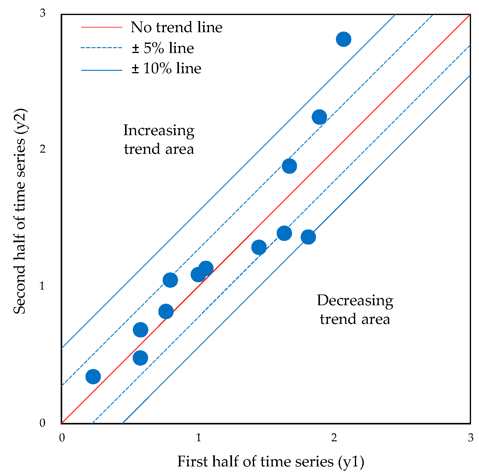
  • Finally, the first part of the data (y1) is located on the x axis and the second part on the y axis (y2) of a Cartesian coordinate system.
Thus, if points are closer to the bisector line (1:1), it can be said that the hydrological time series showed no relevant trend. However, if data points are located above or below the 1:1 line, then increasing or decreasing trends were detected, respectively. It is necessary to define a threshold below or above which a decreasing or increasing trend condition can be defined. In agreement with previous literature studies [32], it is assumed that, if data points are in the ±5–10% range, there was a strong trend, and if data points exceeded ±10%, there was a very strong trend (see Figure 2). Moreover, in order to evaluate the ITA trend’s magnitude, the following equation can be used [33]:
D = 1 n i = 1 n 10 y 2 i y 1 i y 1 ¯
where D is the trend indicator, with positive and negative values indicating increasing or decreasing trends, respectively,   n indicates the number of samples in each subseries, y 1 i and y 2 i are the ith data in the first and second subseries, respectively, and y 1 ¯ is the mean value of the first subseries.

2.5. Modeling Procedure

Overall, the clustering and trends analysis procedure (Figure 3) consists of the following steps:
  • Starting from the time series of the climate variables Tmin, Tmean, Tmax, RHmin, RHmax, Rs, and u5, the PM equation (Equation (1)) was used to calculate the daily ETo for each of the 49 stations located in the Veneto region;
  • The statistical parameters related to both ETo and climate variables were computed for each station;
  • The K-means clustering was employed to identify homogenous regions based on the statistical parameters obtained in step 2;
  • The mean time series of ETo, P and climate variables were computed for each cluster;
  • The seasonal MK test and ITA method were applied to the ETo, P and climate variables’ time series computed for each cluster (step 4) to assess the trends on a monthly scale.
Figure 3. Flowchart of the modeling procedure.
Sustainability 15 11091 g003
Overall, this developed approach, which combines clustering and trend analysis, provides a spatio-temporal characterization of ETo. Additionally, it enables the identification of homogeneous regions and the evaluation of the evolutionary trends of ETo, P, and climate variables.

3. Results

3.1. Clustering

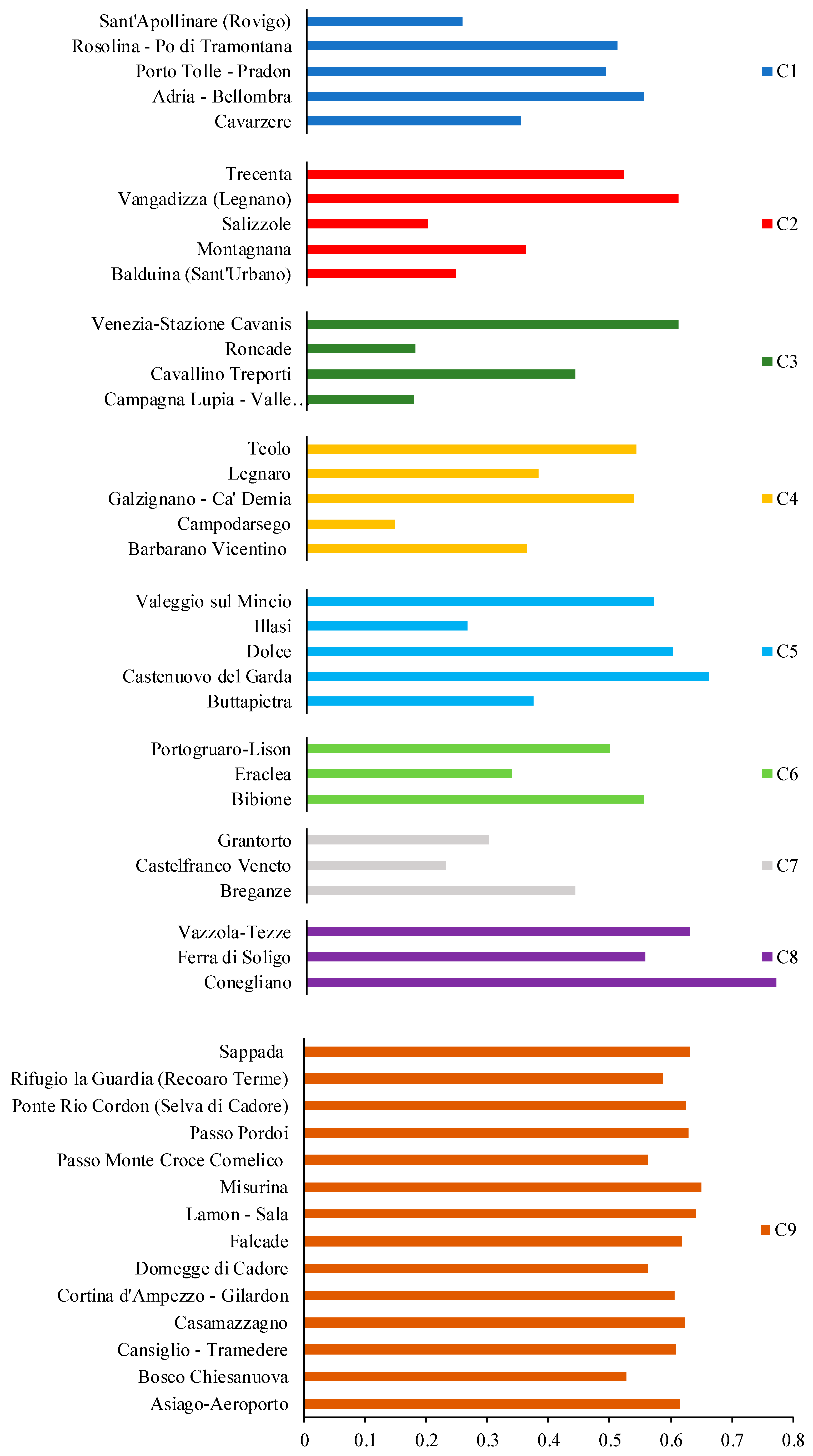
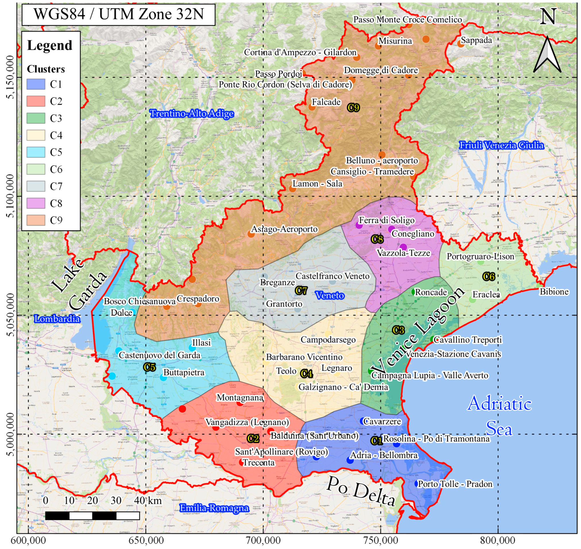
The optimal number of clusters was assessed based on the Silhouette technique described in Section 2.4. As shown in Table 1, the best mean Silhouette score of 0.478, was obtained for nine clusters, including all the statistical parameters in the procedure: ETomean, ETomax, Tmin, Tmean, Tmax, Rs,min, Rs,mean, Rs,max, Vmin, Vmean, and Vmax. The statistics related to each parameter, as well as the mean and maximum daily precipitation (Pmean and Pmax, respectively), and clusters were reported in Table 2. Furthermore, Figure 4 provides the Silhouette scores for all monitoring stations included in the nine clusters, while Figure 5 depicts the clustering of ETo in Veneto. A brief description of the different clusters is provided below:
  • Cluster C1 covers the southern area of the Veneto, including the delta of the Po River, on the border with the Emilia-Romagna region. The area is below the mean sea level (mean altitude equal to −1.20 m.a.s.l.), and is characterized by wetlands, forest, dunes, salt pans, and high biodiversity [34];
  • Cluster C2 is located to the west of cluster C1, and encompasses a portion of the Po Valley characterized by intensive agricultural activity. The main differences between clusters C1 and C2 can be attributed to their distance from the sea. Cluster C1 exhibits higher wind speed, lower maximum temperature, and slightly higher and lower values of the ETomean and of the ETomax, respectively. Cluster C2 had the highest value of maximum temperature among all clusters, reaching Tmax = 39.06 °C;
  • Cluster C3 mainly includes the Venetian Lagoon which consists of mud flats, tidal shallows, and salt marshes, with only a small percentage represented by land [35,36]. Due to its proximity to the Adriatic Sea, cluster C3 is affected by the mitigating effect of the sea, resulting in lower values of Tmax and ETo compared to Cluster C1.
  • Cluster C4 is located to the west of cluster C3 and characterized by a moderately continental climate. It covers a low-plain area subject to intensive agricultural activity, exhibiting similar characteristics to Cluster C2 but with greater windiness due to the Bora winds from the north-east. Cluster C4 has the highest ETomean among all clusters, equal to 2.36 mm/day.
  • Cluster C5 is situated at the western border of Veneto with the Lombardy and Trentino-Alto Adige regions, including a partially mountainous area mitigated by the presence of Lake Garda. This led to the highest mean and maximum Tmean values among all clusters, as well as to the highest value of ETomax;
  • Cluster C6 is located at the border with the Friuli-Venezia Giulia region, to the north-east of the Venice Lagoon, close to the Adriatic Sea. It is an area characterized by a a very low average altitude, equal to 0.33 m, with even stronger winds compared to the Venetian Lagoon (C3), as it is more exposed to the Bora wind from the north-east. Furthermore, compared to cluster C3, both the mean and maximum values of ETo were higher;
  • Cluster C7 is located to the north of cluster C4, in a transition area between the low and flat plains and the mountainous area to the north. However, the mean altitude is still relatively low and equal to 92.33 m above sea level. However, the values of temperature and ETo were slightly lower than those observed in the coastal clusters. Additionally, C7 exhibited the lowest value of the maximum Rs;
  • Cluster C8 is located to the east with respect to cluster C7, at the border with the Friuli-Venezia Giulia region. Although it has similar characteristics to C7, it showed higher Rs and ETo values;
  • Cluster C9 encompasses a large portion of the Northern Veneto, bordering on the west, north, and east with the Trentino-Alto Adige, Austria and Friuli-Venezia Giulia, respectively. It represents the mountainous region of Veneto, including the Venetian Prealps and the Eastern Dolomites, with an average altitude of 1281.93 m above sea level. Consequently, the minimum, mean, and maximum temperatures were significantly lower compared the rest of Veneto, resulting in lower values of ETo as well.
Table 1. Mean Silhouette scores for different numbers of clusters and subsets of input variables (in bold, the best value). Colorbar ranges from red (low values) to green (high values).
Input VariablesNumber of Clusters
23456789101112
ETomean, ETomax, Tmin, Tmean, Tmax, Rs,min, Rs,mean, Rs,max, Vmin, Vmean, Vmax0.4530.4410.4390.4270.430.4650.4720.4780.4760.4530.451
ETomean, ETomax, Tmin, Tmean, Tmax, Rs,min, Rs,mean, Rs,max0.450.4350.4320.4140.4120.4390.450.4610.4630.4580.444
ETomean, ETomax0.4570.4480.4380.4240.4260.4450.4580.4700.4680.4610.448
Table 2. Statistics related to temperature T, altitude, Rs, ETo, V, and P for the different clusters. Colorbar related to T, Rs, V, and P ranges from blue (low values) to red (high values). Altitude colorbar ranges from red (low values) to green (high values). ETo colorbar ranges from light green (low values) to dark green (high values).
C Tmin (°C) Tmean (°C) Tmax (°C) Altitude
MinMeanMaxMinMeanMaxMinMeanMax(m.a.s.l.)
C1−11.669.3924.52−4.9414.0330.26−2.0218.9437.86−1.2
C2−12.388.9124.76−6.213.8630.72−2.419.339.0612.2
C3−8.6510.0326.28−3.8814.1530.68−1.4518.4536.756.5
C4−10.328.8825.44−4.913.8730.96−2.1419.2438.739.4
C5−10.189.1325.48−5.5613.9531.14−2.0219.3438.22105.6
C6−11.139.0824−4.3713.7629.97−1.6318.7337.70.33
C7−10.439.0324.57−4.913.7730.43−2.119.053892.33
C8−9.879.225.47−4.713.8330.8−1.518.8637.8399.67
C9−18.452.417.31−13.76.5623.77−9.9411.6830.851281.93
CRs,minRs,meanRs,maxETomeanETomaxVminVmeanVmaxPmeanPmax
(MJ/m2day)(MJ/m2day)(MJ/m2day)(mm/day)(mm/day)(m/s)(m/s)(m/s)(mm)(mm)
C10.414.1131.782.316.610.262.1914.421.9267.08
C20.1914.0431.42.36.340.041.187.222.0865.72
C30.1714.0631.92.176.070.131.57.92.4767.45
C40.1513.9731.552.366.480.11.578.422.5177.65
C50.0913.5631.122.326.6701.055.162.684.16
C60.0814.0731.662.266.520.231.879.572.8899.13
C70.1313.3730.52.176.060.031.015.33.35104.53
C80.0613.2930.92.196.210.131.084.933.74143.27
C90.0212.2531.71.886.010.041.396.114.05114.67
Moreover, the mean daily precipitation increased from cluster C1 (Pmean = 1.92 mm) to cluster C9 (Pmean = 4.05 mm). The maximum precipitation, on the other hand, exhibited values below 70 mm for clusters C1–C3, ranging between 75 mm and 100 mm for clusters C4–C6, and exceeding 100 mm for clusters C7–C9, with the highest Pmax recorded as 143.27 mm for cluster C8. Overall, the trends in Veneto indicate a climate that becomes progressively wetter, moving from south to north, with higher rainfall observed in the northeastern part of the region.
Figure 4. Silhouette scores for the nine clusters.
Sustainability 15 11091 g004
Figure 5. ETo clustering of Veneto.
Sustainability 15 11091 g005

3.2. ETo and Precipitation Trends Analysis
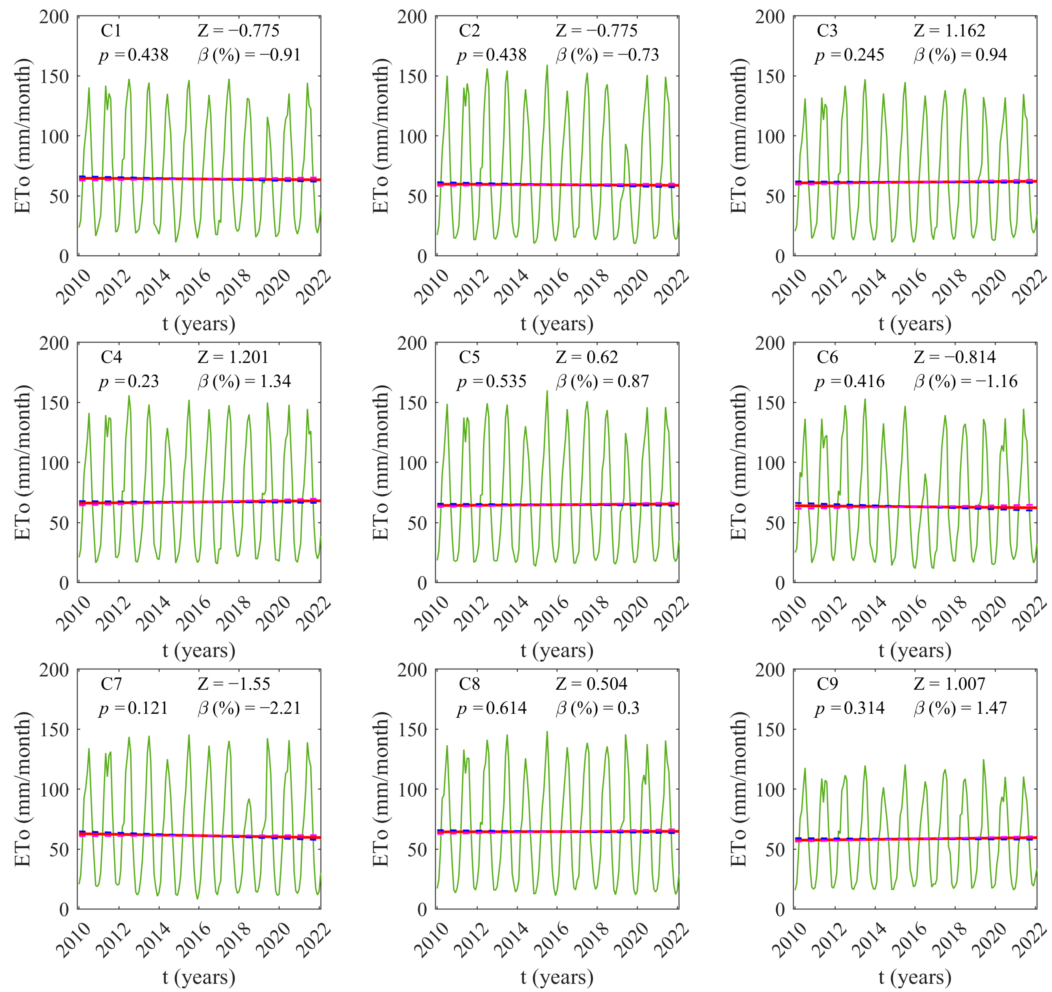
The monthly distribution of Z and β for ETo and P is presented in Figure 6 and Figure 7, respectively. Additionally, the p-values computed using the seasonal MK test are indicated in each plot. These p-values can be used to assess which clusters exhibit significant trends or not. Previous studies on hydrological trends typically consider a threshold value of p (below which trends are considered significant) of 0.05 (e.g., [37]).
Regarding ETo (Figure 6), negative values of both Z and β were calculated for clusters C1, C2, C6, and C7. Specifically, significant decreasing trends were observed in clusters near the Po Delta (C1: Z = −0.755, β = −0.91%; C2: Z = −0. 755, β = −0.73%), as well as for the eastern coastal cluster C6 (Z = −0.814, β = −1.16%). However, the minimum values of Z and β were found in the foothill cluster C7, with Z = −1.550 and β = −2.21%. These distinctive characteristics of C7 can be attributed to its lower temperatures, ETo values and especially to the lowest values of maximum solar radiation compared to all other clusters. Positive values of both Z and β were instead computed for clusters C3, C4, C5, C8, and C9. In particular, the most significant increasing trends were observed for clusters C3 (Z = 1.162, β = 0.94%) and C4 (Z = 1.201, β = 1.34%), which correspond to the Venetian lagoon and to the flat area bordering the lagoon to the northwest. However, the higher value of β was computed for the mountain cluster C9 (Z = 1.007, β = 1.47%), located in the northernmost part of Veneto. Cluster C9, as stated previously, is characterized by the lowest temperature and ETo values among all clusters. Therefore, it appears to be affected by the increase in ETo over the past decade. It must be pointed out that, although significant differences were observed among the nine clusters, no p-values below 0.05 were found, with p ranging from 0.121 (C7) to 0.614 (C8). This means that there are no statistically significant trends.
Figure 6. Distribution of Z and β for ETo on a monthly scale. The red line indicates the median slope while the blue and magenta dashed lines indicate the confidence intervals. Output obtained by the software MATLAB version: 9.13.0 (R2022b) [38].
Sustainability 15 11091 g006
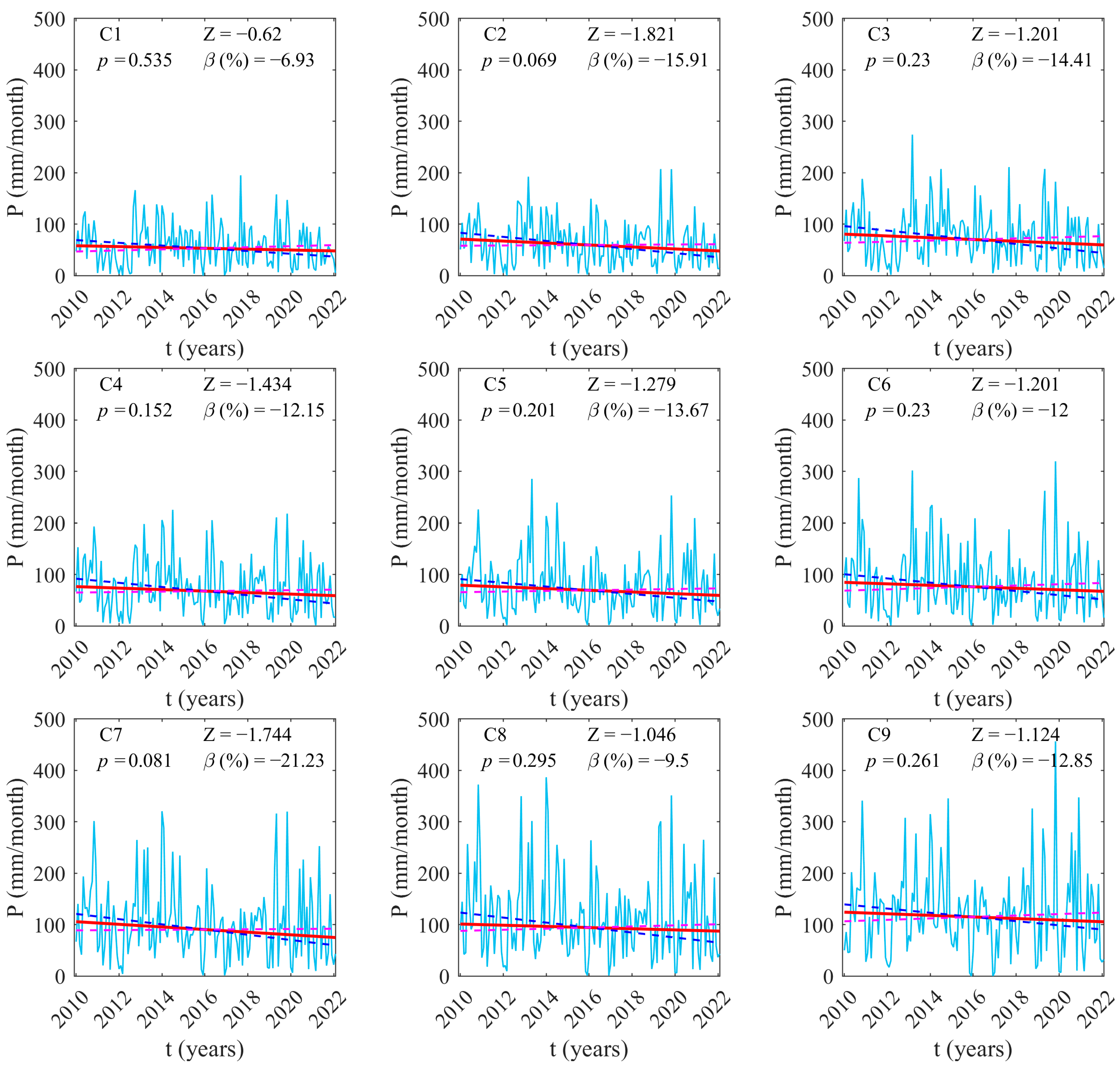
The seasonal MK test for precipitation (Figure 7) revealed negative values of both Z and β for all clusters. Particularly notable decreasing trends were observed in clusters C2 (Z = −0.620, β = −15.91%) and C7 (Z = −1.744, β = −21.23%). This outcome aligns with the ETo analysis, which also indicated lower values of Z and β for clusters C2 and C7. However, discrepancies can be observed for C1, where the values of Z and β computed for P are relatively high compared to the other clusters (Z = −0.620, β = −6.93%). In addition, for clusters C3, C4, C5, C8 and C9, that showed increasing ETo trends, negative Z and β values were computed, with Z ranging between −1.434 (C4) and −1.046 (C8) and β between −14.41% (C3) and −9.50% (C8). Otherwise, C6 showed decreasing trends for P (Z = −1.201, β = −12.00%), in agreement with what was observed for ETo. Moreover, p-values close to 0.05 were computed for cluster C2 and C7 (p equal to 0.069 and 0.081, respectively). For the other cluster, the p-value ranged between 0.152 (C4) and 0.535 (C1).
Figure 7. Distribution of Z and β for P on a monthly scale. The red line indicates the median slope while the blue- and magenta-dashed lines indicate the confidence intervals. Output obtained by the software MATLAB version: 9.13.0 (R2022b) [38].
Sustainability 15 11091 g007
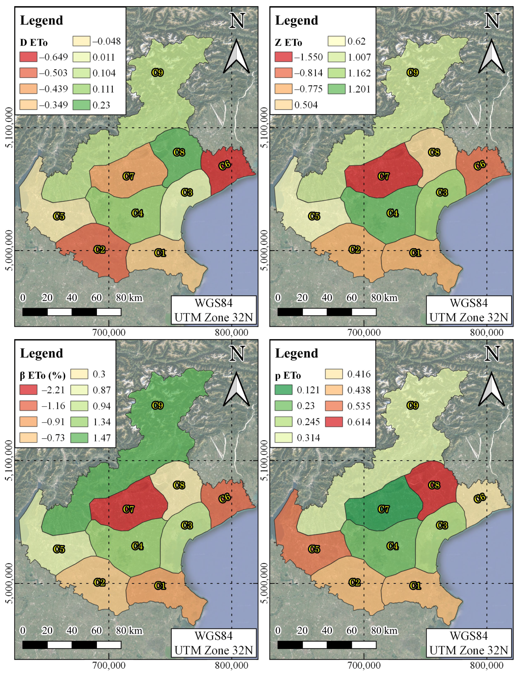
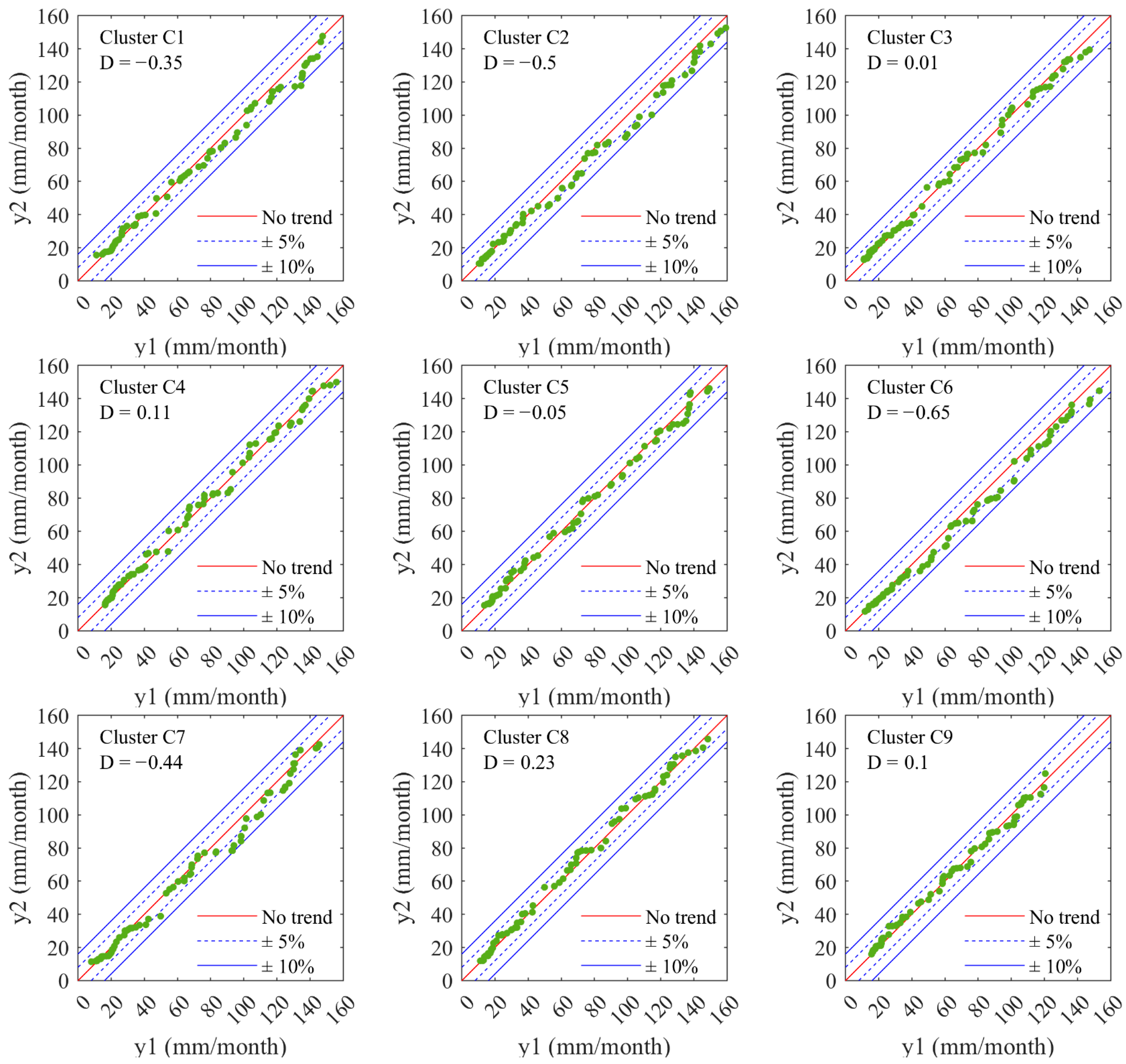
Figure 8 and Figure 9 show the ITA graphs illustrating the monthly ETo and P. Concerning ETo, there was some heterogeneity regarding the value of D among the different clusters. Clusters C1, C2, C5, C6, and C7 exhibited decreasing trends, with C6 showing the lowest D value of −0.65. On the other hand, clusters C3, C4, C8, and C9 showed positive trends, with C8 having the highest D value of 0.23. This finding indicated that D displayed a low sensitivity to the distance from the sea and the land morphology of the region, as both nearshore and inland areas exhibited positive and negative trends. However, upon a detailed analysis of the graphs for each cluster, it was observed that low values of ETo did not exhibit significant trends, with the data points closely aligned to the bisector line (1:1). In contrast, intermediate and high values of ETo displayed deviations from the bisector, moving within the ±5–10% range, indicating more pronounced trends.
In contrast, concerning precipitation, the ITA method revealed greater homogeneity (Figure 9), with decreasing trends observed across all clusters. Specifically, the minimum value of D was computed for cluster C7, equal to −1.48, while C9 showed the higher value of D, equal to −0.49. A further difference in comparison with the trends observed for ETo lies in the lower values of precipitation, where different clusters, such as C2, C4, and C7, showed decreasing trends with data points close to the −5% line. However, in agreement with ETo, the more marked decreasing trends were observed for the higher values of precipitation, with data points close or below the −10% line (e.g., clusters C7 and C8).
Figure 9. Results of ITA for monthly P at the 9 clusters. Output obtained by the software MATLAB version: 9.13.0 (R2022b) [38].
Sustainability 15 11091 g009
A comparison between the outcomes of the seasonal MK test and ITA method was also performed. Figure 10 illustrates the spatial distribution of the ITA and MK parameters evaluated on monthly ETo. In addition, a correlation matrix has been provided in Table 3 showing the correlation coefficient R between the ITA and the MK parameters evaluated on both ETo and P. The spatial distributions of the Z and β parameters computed for the MK test exhibited notable agreement. Consequently, the correlation between these parameters was strong, with R values exceeding 0.862 for P and 0.980 for ETo. Comparing the parameter D of the ITA method with the MK test parameters, different similarities were observed. This resulted in a correlation between D, Z, and β, ranging equal to or higher than 0.834 for ETo and 0.720 for P, which is relatively high. Regarding the p-value, low correlations were observed for ETo, with values equal to 0.073 and 0.131 between Z and p and between β and p, respectively. Conversely, for precipitation, the p-value is strongly correlated with Z and β, with correlations equal to 0.967 and 0.837, respectively.
A further comparison was performed between the ITA method and the MK test parameters calculated for both ETo and P. Low correlations were observed between the D values computed for ETo and P (R = 0.192). The MK test parameters computed for both ETo and P also showed low correlation, ranging between 0.063 and 0.613.
Figure 10. Spatial distribution of the ITA and seasonal MK parameters evaluated on the ETo time series. For D, Z, and β, colorbar ranges from red (low values) to green (high values). For the p-values, colorbar ranges from green (low values) to red (high values).
Sustainability 15 11091 g010
Table 3. Correlation matrix of the ITA and seasonal MK parameters evaluated on both ETo and P. Colorbar ranges from red (low values) to green (high values).
Correlation MatrixITAMK
EToPEToP
DDZβpZβp
ITAEToD1.0000.1920.8710.8340.1260.2780.2900.138
PD0.1921.0000.1890.2700.2150.7200.7200.703
MKEToZ0.8710.1891.0000.9800.0730.2450.3130.063
β0.8340.2700.9801.0000.1310.2390.3410.073
p0.1260.2150.0730.1311.0000.4080.6130.386
PZ0.2780.7200.2450.2390.4081.0000.8620.967
β0.2900.7200.3130.3410.6130.8621.0000.837
p0.1380.7030.0630.0730.3860.9670.8371.000

3.3. Climate Variables Trends Analysis

The trends of climate variables were discussed in this section, providing the parameters of the seasonal MK test and ITA method, for ETo, P, and climate variables, in Table 4. In addition, in order to compare the trends observed for the climate variables with those of ETo and P, a correlation matrix is provided in Table 5.
Regarding temperature, the MK test showed positive trends for some clusters and negative trends for others. In particular, cluster C7 was the only one with a negative Z and β values for all three temperature parameters, namely Tmin, Tmea, and Tmax. Cluster C1 also showed negative Z and β values for Tmin and Tmean, while highlighting positive values for Tmax. More generally, with the exception of C7, all clusters show increasing values of Z and β for Tmax. For Tmin, on the other hand, there were discrepancies, with C1, C2, C4 and C7 showing negative trends. The MK test outcomes were quite in agreement with the ITA method. In particular, both clusters C1 and C7 showed a negative D for all three temperature parameters, with Tmin being confirmed as the one with the greatest discrepancies among the various clusters, with the negative D for C1, C2, C6, C7, and C8. Moreover, the correlation between the seasonal MK test and ITA method parameters computed for ETo with those observed for the three temperatures were quite high, with values up to 0.739, 0.768 and 0.637 for Z, β and D, respectively.
Relative humidity showed discrepancies between minimum (RHmin) and maximum (RHmax) values. Specifically, while for RHmax, both the ITA method and MK test showed markedly positive D, Z and B values for all clusters, for RHmin, C4 and C7 (and also C8 for the ITA method) showed negative trends. Moreover, for RHmax, the p-values were lower than 0.05 for all clusters, confirming statistically significant positive trends. In addition, C6 and C9 also exhibited statistically significant positive trends for RHmin. The correlation between Z, β, and D computed for ETo and both RHmax and RHmin were negative, with values up to −0.729, −0.221 and −0.571 for Z, β and D, respectively.
Solar radiation highlighted positive trends for all clusters and for both the MK test and ITA method, with the highest and lowest values of Z, β and D for C8 and C6, respectively. In addition, p-values were lower than 0.05 for all clusters, with the exception of C6 and C9, highlighting statistically significant trends. The correlation between D computed for ETo and Rs was also quite high and equal to 0.684, while the correlation between Z and β, computed for ETo and Rs, was low and equal to 0.081 and −0.053, respectively.
Regarding the wind velocity, the seasonal MK test showed positive trends for C2, C5, C8, and C9, with C5 and C6 that exhibited the more marked positive and negative values of Z and β, respectively. Furthermore, statistically significant trends (p-values < 0.05) were observed for C1, C4, C5, C6, and C8. The ITA method was quite in agreement with the MK test, with the exception of C7, for which the highest value of D among all clusters was computed. In this case, the correlations between Z, β, and D computed for ETo and u5 were quite low with values equal to 0.302, 0.352, and −0.157, respectively.
Table 4. Seasonal MK and ITA method parameters computed for ETo, P and climate variables. For D, Z and β, the colorbar ranges from red (low values) to green (high values). For the p-values, the colorbar ranges from green (low values) to red (high values).
C1C2C3C4C5C6C7C8C9
DETo−0.349−0.5030.0110.111−0.048−0.649−0.4390.2300.104
P0.4380.4380.2450.2300.5350.4160.1210.6140.314
Tmin−0.455−0.4130.0420.0280.121−0.077−0.712−0.0450.633
Tmean−0.172−0.0230.1660.1430.2130.111−0.3910.0760.335
Tmax−0.0230.1270.2080.2190.2310.196−0.2530.0870.343
RHmin0.1120.2800.140−0.0810.1260.378−0.116−0.2340.339
RHmax0.1420.2550.0910.1080.1700.1940.1550.1350.188
Rs0.3000.2480.2730.3890.3700.1020.3630.4820.265
u5−0.6070.148−0.391−1.8671.057−0.6363.5410.8420.424
ZETo−0.775−0.7751.1621.2010.620−0.814−1.5500.5041.007
P−0.620−1.821−1.201−1.434−1.279−1.201−1.744−1.046−1.124
Tmin−0.814−0.3100.232−0.0580.8140.194−1.0070.3490.852
Tmean−0.1551.1621.5110.6970.9301.162−0.4650.7751.046
Tmax0.9691.3171.8211.2011.2401.434−0.3100.6201.395
RHmin1.0071.0851.472−0.6591.1242.054−0.2130.0391.976
RHmax5.6574.9213.1593.5653.2175.3473.9733.5263.565
Rs2.6742.3252.3642.9452.4801.4722.6742.9841.627
u5−2.4410.078−0.891−2.4413.275−3.487−0.4261.9370.969
β (%)ETo−0.91−0.730.941.340.87−1.16−2.210.301.47
P−6.93−15.91−14.41−12.15−13.67−12.00−21.23−9.50−12.85
Tmin−0.22−0.080.06−0.030.240.05−0.300.080.23
Tmean−0.050.350.360.220.440.40−0.220.140.31
Tmax0.380.600.590.540.520.54−0.200.230.58
RHmin1.291.591.08−0.891.682.63−0.150.063.52
RHmax1.521.891.191.342.112.061.862.022.02
Rs0.550.550.560.650.680.390.680.760.35
u5−0.140.00−0.03−0.100.08−0.18−0.010.050.03
pETo0.4380.4380.2450.2300.5350.4160.1210.6140.314
P0.5350.0690.2300.1520.2010.2300.0810.2950.261
Tmin0.4160.7570.8160.9540.4160.8460.3140.7270.394
Tmean0.8770.2450.1310.4850.3520.2450.6420.4380.295
Tmax0.3330.1880.0690.2300.2150.1520.7570.5350.163
RHmin0.3140.2780.1410.5100.2610.0400.8310.9690.048
RHmax<0.001<0.0010.002<0.0010.001<0.001<0.001<0.001<0.001
Rs0.0080.0200.0180.0030.0130.1410.0080.0030.104
u50.0150.9380.3730.0150.001<0.0010.6700.0530.333
Table 5. Correlation matrix of the ITA and seasonal MK parameters evaluated on ETo, P, and climate variables. Colorbar ranges from red (low values) to green (high values).
Correlation MatrixDZβ (%)p
EToPEToPEToPEToP
DTmin0.6370.1650.8180.2980.8600.3090.1650.100
Tmean0.5560.2980.8280.2320.8690.3550.2980.034
Tmax0.4320.2710.7640.1950.8260.3680.2710.025
RHmin−0.4560.035−0.0710.0370.0370.0370.0350.026
RHmax−0.5710.288−0.487−0.398−0.341−0.2190.288−0.312
Rs0.6840.1490.3050.0130.2590.0430.1490.008
u5−0.157−0.148−0.474−0.379−0.494−0.662−0.148−0.328
ZTmin0.5610.4080.7390.1880.7740.2360.408−0.025
Tmean0.2380.2700.591−0.0550.5970.1250.270−0.212
Tmax0.1510.2040.5780.2530.6170.3950.2040.148
RHmin−0.2840.2190.0190.2990.0870.1710.2190.246
RHmax−0.7950.156−0.7290.192−0.6640.2860.1560.356
Rs0.3890.0450.081−0.0320.0150.0630.0450.041
u50.4960.4320.302−0.1240.345−0.1650.432−0.183
β (%)Tmin0.5360.4310.7270.1970.7680.2490.431−0.009
Tmean0.1450.3650.536−0.0360.5850.1630.365−0.189
Tmax0.1520.2810.5610.1960.6380.4290.2810.109
RHmin−0.2390.237−0.0030.2470.1070.1430.2370.204
RHmax−0.2010.507−0.310−0.132−0.221−0.1060.507−0.162
Rs0.3380.1660.028−0.179−0.053−0.1140.166−0.153
u50.5260.2410.325−0.2750.352−0.3230.241−0.327
pTmin0.0830.0520.334−0.1370.2650.2080.052−0.222
Tmean−0.117−0.058−0.4320.344−0.4190.245−0.0580.502
Tmax−0.065−0.131−0.520−0.180−0.577−0.322−0.131−0.087
RHmin0.2500.036−0.189−0.184−0.273−0.1520.036−0.135
RHmax0.270−0.1030.4670.0690.381−0.129−0.103−0.030
Rs−0.3290.001−0.0720.122−0.0270.0730.0010.025
u5−0.356−0.374−0.391−0.731−0.361−0.724−0.374−0.604

4. Discussion

The spatial-temporal analysis of ETo in Veneto yielded the following findings:
  • The clustering procedure divided Veneto into nine clusters. Clusters C1, C3, and C6 cover the coastal area, ranging from the Po Delta (C1) to the Venetian Lagoon (C3) and bordering Friuli-Venezia Giulia (C6). Clusters C2, C4, C5, C7, and C8 encompass the flat area, extending from the Po Valley (C2), to the Garda Lake in the west (C5) and the foothills area bordering Friuli-Venezia Giulia in the east (C8). Lastly, cluster C9 covers the northern mountainous portion of Veneto, encompassing the Venetian Prealps and the Eastern Dolomites.
  • Each cluster exhibited distinct values of the analyzed climate variables. For instance, the coastal cluster C1 displayed higher wind velocity, while C2 and C5 had the highest values of Tmax and ETo, respectively. Conversely, the mountainous cluster C9 exhibited the lowest values of temperature and ETo. Additionally, the mean daily precipitation increased from cluster C1 to C9, with higher rainfall in the northeastern part of Veneto, spanning clusters C7–C9.
  • According to the MK test, ETo trends are decreasing for the coastal clusters C1 and C6, but also for C2, near the Po River, and the foothill cluster C7. In contrast, increasing trends were observed for the coastal cluster C3, which include the Venice Lagoon, and for the inland cluster C4, C5, C8, and C9. Precipitation exhibited negative trends for all clusters, with the more marked decreasing trends observed for C2 and C7, in agreement with what was observed for ETo.
  • Conversely, the ITA method indicated positive ETo trends for clusters C3, C4, C8, and C9, in agreement with what was observed with the MK test. In addition, both methods agreed on decreasing trends in precipitation for all clusters. Moreover, the ITA method revealed more pronounced trends for intermediate and high values of ETo and precipitation, while no relevant trends were observed for the low values of both variables.
  • The climate parameters Tmax, RHmax, and Rs exhibited increasing trends for all clusters, suggesting a gradual warming of the Veneto region. This warming trend significantly impacts evapotranspiration and, consequently, will have deep implications for the future management of water resources for different purposes.
In the present study, decreasing trends in P and ETo were observed for the coastal clusters characterized by a Mediterranean climate. These results were in disagreement with Chaouche et al. [10], which reported no significant P trends but increasing ETo trends for the Mediterranean coastal area of France. On the other hand, the decrease in precipitation observed for the inland clusters, characterized by a moderate continental climate, was in agreement with what was observed by Prăvălie et al. [18] for the continental climate of Romania. However, the latter study also reported general ETo increases in disagreement with the present study. Regarding to the precipitation, Aschale et al. [11] also observed a downward trend for Sicily with, however, no relevant ETo trends. The discrepancies between the various works can be attributed to numerous factors that may relate on the one hand to the length of the time series and on the other hand to the peculiar aspects of each study area with morphology and micro-climates that can result in different evidence in areas with apparently similar features.
It should be noted that the importance of analyzing ETo and rainfall trends is even greater in the light of climate change. In particular, in Veneto, agriculture plays a significant role in the regional economy, occupying an area larger than 800,000 hectares. Veneto’s agricultural sector is among the most productive in Italy [39]. Major agricultural products include grain crops, particularly in the southern and eastern parts of the region, as well as fruits and wine, which are widespread in the plains and foothills. However, the impacts of climate change on the hydrological cycle have been observed in recent decades, exacerbated by increased irrigation demands. Veneto has experienced average temperature increases in both the winter and summer seasons. Simultaneously, the decreasing precipitation trends shown in the present study, along with a concentration of precipitation in a reduced number of rainfall events, is leading to the more frequent occurrences of floods and droughts [40,41]. Reduced rainfall can lead to a decrease in groundwater levels, impacting the availability of water for domestic, agricultural and industrial purposes, as well as affecting the distribution and composition of plant and animal species, with potential damage to ecosystems. Moreover, rising sea levels associated with climate change can lead to both the saltwater intrusion into coastal aquifers and an increased risk of flooding for the entire Veneto’s coastline, including Venice and its lagoon [35,36].
It must be pointed out that, although Veneto exhibits different local climates, ranging from coastal to mountainous areas, a limitation of the present study is the lack of consideration for different climates, such as arid or semi-arid regions, where larger or smaller variations in ETo may occur throughout the seasons. Additionally, in future research, the implemented methodology could be applied to investigate trends related to crop evapotranspiration, considering the typical crops grown in the different areas of Veneto, each characterized by varying water demands. This approach would provide further insights into similarities and differences in clustering and trends related to reference and crop evapotranspiration.

5. Conclusions

This study showed an extensive spatio-temporal analysis of ETo in Veneto. Data recorded from 49 stations across Veneto were utilized to evaluate ETo using the Penman–Monteith equation. The K-means algorithm was employed to divide the study area into nine homogeneous regions, each characterized by particular ETo features. Additionally, the seasonal MK test and ITA method were used to identify trends in the ETo and P time series on a monthly scale for each cluster. Overall, the MK test revealed decreasing trends in precipitation for all clusters, with the clusters C2, located near the Po Delta, and the foothill cluster C7. The MK test also showed decreasing ETo trends for different clusters, including C2 and C7. However, the coastal cluster C3 and the inland cluster C4, C5, C8, and C9 showed increasing trends. At the same time, the ITA method revealed positive ETo trends for clusters C3, C4, C8, and C9, in agreement with the seasonal MK test, while the remaining clusters exhibited negative trends. Also consistent with the MK test, the ITA method identified negative trends in P for all clusters. Furthermore, ITA highlighted more pronounced trends for higher values of both ETo and P, while lower values showed no significant trends. This suggests considerable variations in extreme values of precipitation and ETo. Moreover, the increasing trends observed for Tmax, RHmax, Rs confirm the gradual warming of the climate in Veneto. The developed approach, combining clustering methods and trend analysis, aims to provide a concise and reliable evaluation of the ETo evolutionary trends, along with the identification of different homogeneous regions. Consequently, this approach can be a useful decision-making tool for water resource management, accounting for the diverse morpho-climatic characteristics within a water district as well as to the temporal evolution of meteorological variables.

Author Contributions

Conceptualization, F.D.N. and F.G.; methodology, F.D.N. and F.G.; software, F.D.N. and F.G.; validation, F.D.N. and F.G.; data curation, M.D.M. and G.I.; writing—original draft preparation, F.D.N. and F.G.; writing—review and editing, F.D.N. and F.G.; visualization, F.D.N., M.D.M., G.I. and F.G.; supervision, F.G. All authors have read and agreed to the published version of the manuscript.

Funding

This research received no external funding.

Institutional Review Board Statement

Not applicable.

Informed Consent Statement

Not applicable.

Data Availability Statement

The data are available on the ARPAV website: https://wwwold.arpa.veneto.it/arpavinforma/bollettini (accessed on 13 July 2023).

Conflicts of Interest

The authors declare no conflict of interest.

References

  1. Granata, F. Evapotranspiration evaluation models based on machine learning algorithms—A comparative study. Agric. Water Manag. 2019, 217, 303–315. [Google Scholar] [CrossRef]
  2. Allen, R.G.; Pereira, L.S.; Raes, D.; Smith, M. Crop Evapotranspiration: Guidelines for Computing Crop Water Requirements; Food and Agriculture Organization of the United Nations: Rome, Italy, 1998. [Google Scholar]
  3. Xing, W.; Wang, W.; Shao, Q.; Yu, Z.; Yang, T.; Fu, J. Periodic fluctuation of reference evapotranspiration during the past five decades: Does evaporation paradox really exist in China. Sci. Rep. 2016, 6, 39503. [Google Scholar] [CrossRef] [PubMed] [Green Version]
  4. Masanta, S.K.; Vemavarapu, S.V. Regionalization of evapotranspiration using fuzzy dynamic clustering approach. Part 1: Formation of regions in India. Int. J. Climatol. 2020, 40, 3514–3530. [Google Scholar] [CrossRef]
  5. Chen, Z.; Zhu, Z.; Jiang, H.; Sun, S. Estimating daily reference evapotranspiration based on limited meteorological data using deep learning and classical machine learning methods. J. Hydrol. 2020, 591, 125286. [Google Scholar] [CrossRef]
  6. Mann, H.B. Nonparametric tests against trend. Econometrica 1945, 13, 245–259. [Google Scholar] [CrossRef]
  7. Kendall, M.G. Rank Correlation Methods; Griffin: New York, NY, USA, 1948; p. 202. [Google Scholar]
  8. Sen, Z. Innovative trend analysis methodology. J. Hydrol. Eng. 2012, 17, 1042–1046. [Google Scholar] [CrossRef]
  9. Granata, F.; Di Nunno, F. Forecasting evapotranspiration in different climates using ensembles of recurrent neural networks. Agric. Water Manag. 2021, 255, 107040. [Google Scholar] [CrossRef]
  10. Chaouche, K.; Neppel, L.; Dieulin, C.; Pujol, N.; Ladouche, B.; Martin, E.; Salas, D.; Caballero, Y. Analyses of precipitation, temperature and evapotranspiration in a French Mediterranean region in the context of climate change. Comptes Rendus Geosci. 2010, 342, 234–243. [Google Scholar] [CrossRef]
  11. Aschale, T.M.; Peres, D.J.; Gullotta, A.; Sciuto, G.; Cancelliere, A. Trend Analysis and Identification of the Meteorological Factors Influencing Reference Evapotranspiration. Water 2023, 15, 470. [Google Scholar] [CrossRef]
  12. Di Nunno, F.; Granata, F. Future trends of reference evapotranspiration in Sicily based on CORDEX data and Machine Learning algorithms. Agric. Water Manag. 2023, 280, 108232. [Google Scholar] [CrossRef]
  13. Pandey, B.K.; Khare, D. Identification of trend in long term precipitation and reference evapotranspiration over Narmada River basin (India). Glob. Planet. Chang. 2018, 161, 172–182. [Google Scholar] [CrossRef]
  14. Jerin, J.N.; Islam, H.M.T.; Islam, A.R.M.T.; Shahid, S.; Hu, Z.; Badhan, M.A.; Chu, R.; Elbeltagi, A. Spatiotemporal trends in reference evapotranspiration and its driving factors in Bangladesh. Theor. Appl. Climatol. 2021, 144, 793–808. [Google Scholar] [CrossRef]
  15. Xu, S.; Yu, Z.; Yang, C.; Ji, X.; Zhang, K. Trends in evapotranspiration and their responses to climate change and vegetation greening over the upper reaches of the Yellow River Basin. Agric. For. Meteorol. 2018, 263, 118–129. [Google Scholar] [CrossRef]
  16. Li, Y.; Yao, N.; Chau, H.W. Influences of removing linear and nonlinear trends from climatic variables on temporal variations of annual reference crop evapotranspiration in Xinjiang, China. Sci. Total Environ. 2017, 592, 680–692. [Google Scholar] [CrossRef] [PubMed] [Green Version]
  17. Fu, J.; Gong, Y.; Zheng, W.; Zou, J.; Zhang, M.; Zhang, Z.; Qin, J.; Liu, J.; Quan, B. Spatial-temporal variations of terrestrial evapotranspiration across China from 2000 to 2019. Sci. Total Environ. 2022, 825, 153951. [Google Scholar] [CrossRef] [PubMed]
  18. Kişi, O. An innovative method for trend analysis of monthly pan evaporations. J. Hydrol. 2015, 527, 1123–1129. [Google Scholar] [CrossRef]
  19. Prăvălie, R.; Piticar, A.; Roșca, B.; Sfîcă, L.; Bandoc, G.; Tiscovschi, A.; Patrich, C. Spatio-temporal changes of the climatic water balance in Romania as a response to precipitation and reference evapotranspiration trends during 1961–2013. CATENA 2019, 172, 295–312. [Google Scholar] [CrossRef]
  20. Zolin, M.B.; Pastore, A.; Mazzarolo, M. Common agricultural policy and sustainable management of areas with natural handicaps. The Veneto Region case study. Environ. Dev. Sustain. 2020, 22, 7587–7605. [Google Scholar] [CrossRef]
  21. Barbi, A.; Cagnati, A.; Cola, G.; Checchetto, F.; Chiaudani, A.; Crepaz, A.; Delillo, I.; Mariani, L.; Marigo, G.; Meneghin, P.; et al. Atlante Climatico del Veneto. Precipitazioni—Basi Informative per l’analisi Delle Correlazioni tra Cambiamenti Climatici e Dinamiche Forestali nel Veneto 2013. Regione del Veneto, Mestre. Available online: https://www.arpa.veneto.it/temi-ambientali/agrometeo/approfondimenti/atlante-agroclimatico-veneto-precipitazioni (accessed on 13 July 2023).
  22. Zotarelli, L.; Dukes, M.D.; Romero, C.C.; Migliaccio, K.W.; Morgan, K.T. Step by Step Calculation of the Penman-Monteith Evapotranspiration (FAO-56 Method). Doc. AE459, University of Florida. 2010. Available online: https://www.agraria.unirc.it/documentazione/materiale_didattico/1462_2016_412_24509.pdf (accessed on 13 July 2023).
  23. Barton, Y.; Giannakaki, P.; Von Waldow, H.; Chevalier, C.; Pfahl, S.; Martius, O. Clustering of regional-scale extreme precipitation events in southern Switzerland. Mon. Weather Rev. 2016, 144, 347–369. [Google Scholar] [CrossRef] [Green Version]
  24. Di Nunno, F.; Granata, F. Spatio-temporal analysis of drought in Southern Italy: A combined clustering-forecasting approach based on SPEI index and artificial intelligence algorithms. Stoch. Environ. Res. Risk Assess. 2023, 37, 2349–2375. [Google Scholar] [CrossRef]
  25. Demsar, J.; Curk, T.; Erjavec, A.; Gorup, C.; Hocevar, T.; Milutinovic, M.; Mozina, M.; Polajnar, M.; Toplak, M.; Staric, A.; et al. Orange: Data Mining Toolbox in Python. J. Mach. Learn. Res. 2013, 14, 2349–2353. [Google Scholar]
  26. Callahan, C.; Bridge, H. Data Mining of Rare Alleles to Assess Biogeographic Ancestry. In Proceedings of the 2021 Systems and Information Engineering Design Symposium (SIEDS), Charlottesville, VA, USA, 29–30 April 2021; 1–6. [Google Scholar] [CrossRef]
  27. Wang, F.; Shao, W.; Yu, H.; Kan, G.; He, X.; Zhang, D.; Ren, M.; Wang, G. Re-evaluation of the Power of the Mann-Kendall Test for Detecting Monotonic Trends in Hydrometeorological Time Series. Front. Earth Sci. 2020, 8, 14. [Google Scholar] [CrossRef]
  28. Wang, L.; Akritas, M.G.; Van Keilegom, I. An ANOVA-Type Nonparametric Diagnostic Test for Heteroscedastic Regression Models. J. Nonparametr. Stat. 2008, 20, 365–382. [Google Scholar] [CrossRef]
  29. Umar, D.A.; Ramli, M.F.; Aris, A.Z.; Jamil, N.R.; Abdulkareem, J.H. Runoff irregularities, trends, and variations in tropical semi-arid river catchment. J. Hydrol. Reg. Stud. 2018, 19, 335–348. [Google Scholar] [CrossRef]
  30. Meggiorin, M.; Passadore, G.; Bertoldo, S.; Sottani, A.; Rinaldo, A. Assessing the long-term sustainability of the groundwater resources in the Bacchiglione basin (Veneto, Italy) with the Mann–Kendall test: Suggestions for higher reliability. Acque Sotter.-Ital. J. Groundw. 2021, 10, 35–48. [Google Scholar] [CrossRef]
  31. Ashraf, M.S.; Ahmad, I.; Khan, N.M.; Zhang, F.; Bilal, A.; Guo, J. Streamflow Variations in Monthly, Seasonal, Annual and Extreme Values Using Mann-Kendall, Spearmen’s Rho and Innovative Trend Analysis. Water Resour. Manag. 2021, 35, 243–261. [Google Scholar] [CrossRef]
  32. Gumus, V.; Avsaroglu, Y.; Simsek, O. Streamflow trends in the Tigris river basin using Mann−Kendall and innovative trend analysis methods. J. Earth Syst. Sci. 2022, 131, 34. [Google Scholar] [CrossRef]
  33. Wu, H.; Qian, H. Innovative trend analysis of annual and seasonal rainfall and extreme values in Shaanxi, China, since the 1950s. Int. J. Climatol. 2017, 37, 2582–2592. [Google Scholar] [CrossRef]
  34. Corbau, C.; Simeoni, U.; Zoccarato, C.; Mantovani, G.; Teatini, P. Coupling land use evolution and subsidence in the Po Delta, Italy: Revising the past occurrence and prospecting the future management challenges. Sci. Total Environ. 2019, 654, 1196–1208. [Google Scholar] [CrossRef]
  35. Granata, F.; Di Nunno, F. Artificial Intelligence models for prediction of the tide level in Venice. Stoch. Environ. Res. Risk Assess. 2021, 35, 2537–2548. [Google Scholar] [CrossRef]
  36. Di Nunno, F.; Granata, F.; Gargano, R.; de Marinis, G. Forecasting of Extreme Storm Tide Events Using NARX Neural Network-Based Models. Atmosphere 2021, 12, 512. [Google Scholar] [CrossRef]
  37. Peña-Angulo, D.; Vicente-Serrano, S.M.; Domínguez-Castro, F.; Lorenzo-Lacruz, J.; Murphy, C.; Hannaford, J.; Allan, R.P.; Tramblay, Y.; Reig-Gracia, F.; El Kenawym, A. The complex and spatially diverse patterns of hydrological droughts across Europe. Water Resour. Res. 2022, 58, e2022WR031976. [Google Scholar] [CrossRef]
  38. The MathWorks Inc. Optimization Toolbox, version: 9.0.13 (R2022b); The MathWorks Inc.: Natick, MA, USA, 2022; Available online: https://www.mathworks.com (accessed on 13 July 2023).
  39. Vanni, F.; Povellato, A. Delivering public goods through agriculture. Some evidence from viticulture in Veneto region. In Proceedings of the International Conference “Enometrics XVII”, Palermo, Italy, 9–12 June 2010. [Google Scholar]
  40. Sofia, G.; Roder, G.; Dalla Fontana, G.; Tarolli, P. Flood dynamics in urbanised landscapes: 100 years of climate and humans’ interaction. Sci. Rep. 2017, 7, 40527. [Google Scholar] [CrossRef] [PubMed]
  41. Salpina, D.; Pagliacci, F. Are We Adapting to Climate Change? Evidence from the High-Quality Agri-Food Sector in the Veneto Region. Sustainability 2022, 14, 11482. [Google Scholar] [CrossRef]
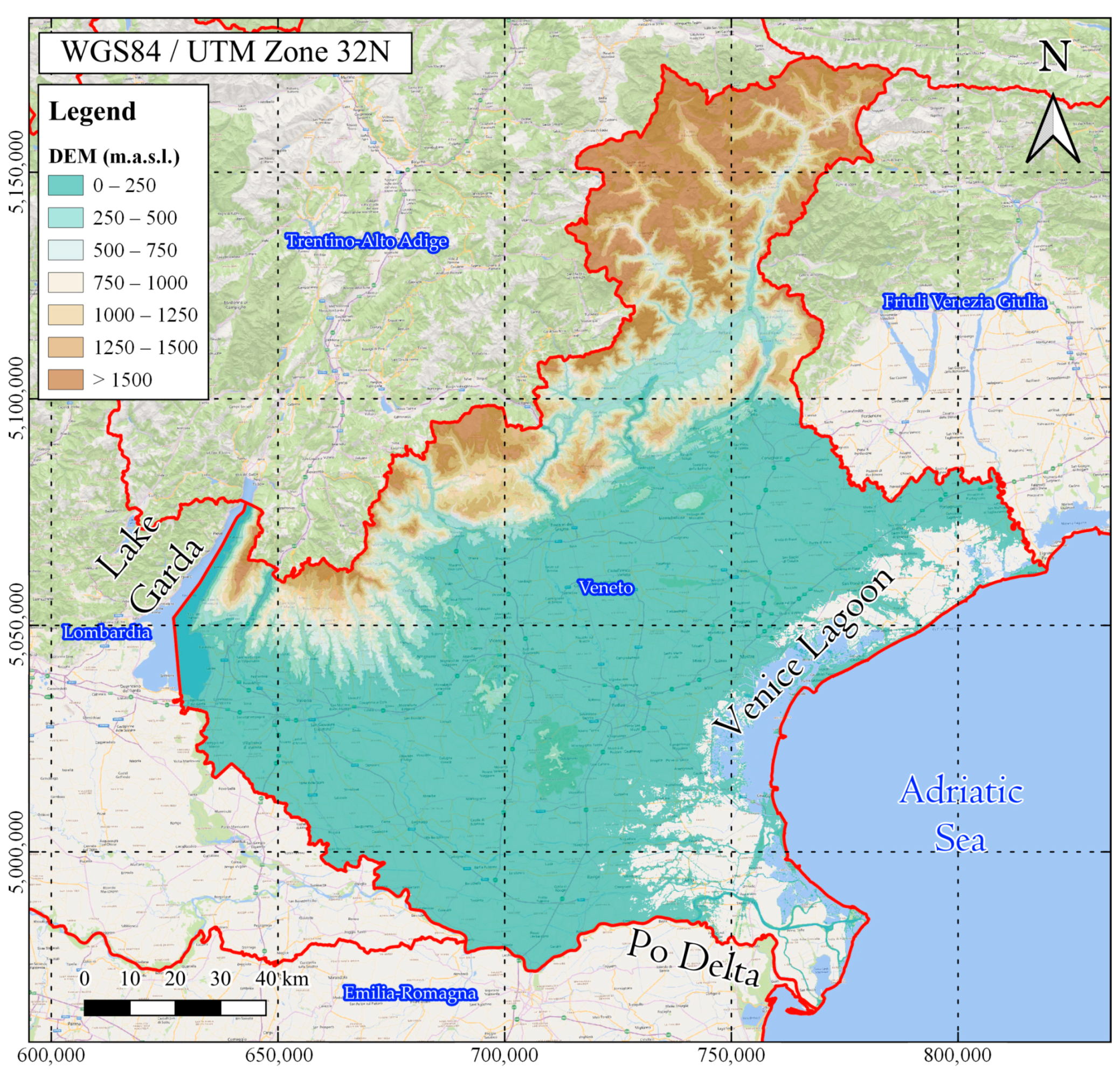
Figure 1. Location of the stations in Veneto with a digital elevation model (DEM) representation.
Sustainability 15 11091 g001
Figure 2. Representation of the ITA method, with an indication of the increasing and decreasing trend areas.
Sustainability 15 11091 g002
Figure 8. Results of ITA for monthly ETo at the 9 clusters. Output obtained by the software MATLAB version: 9.13.0 (R2022b) [38].
Sustainability 15 11091 g008
Disclaimer/Publisher’s Note: The statements, opinions and data contained in all publications are solely those of the individual author(s) and contributor(s) and not of MDPI and/or the editor(s). MDPI and/or the editor(s) disclaim responsibility for any injury to people or property resulting from any ideas, methods, instructions or products referred to in the content.