Short-Term Power Load Forecasting in Three Stages Based on CEEMDAN-TGA Model

Abstract

Short-term load forecasting (STLF) is crucial for intelligent energy and power scheduling. The time series of power load exhibits high volatility and complexity in its components (typically seasonality, trend, and residuals), which makes forecasting a challenge. To reduce the volatility of the power load sequence and fully explore the important information within it, a three-stage short-term power load forecasting model based on CEEMDAN-TGA is proposed in this paper. Firstly, the power load dataset is divided into the following three stages: historical data, prediction data, and the target stage. The CEEMDAN (complete ensemble empirical mode decomposition with adaptive noise) decomposition is applied to the first- and second-stage load sequences, and the reconstructed intrinsic mode functions (IMFs) are classified based on their permutation entropies to obtain the error for the second stage. After that, the TCN (temporal convolutional network), GRU (gated recurrent unit), and attention mechanism are combined in the TGA model to predict the errors for the third stage. The third-stage power load sequence is predicted by employing the TGA model in conjunction with the extracted trend features from the first and second stages, as well as the seasonal impact features. Finally, it is merged with the error term. The experimental results show that the forecast performance of the three-stage forecasting model based on CEEMDAN-TGA is superior to those of the TCN-GRU and TCN-GRU-Attention models, with a reduction of 42.77% in MAE, 46.37% in RMSE, and 45.0% in MAPE. In addition, the R² could be increased to 0.98. It is evident that utilizing CEEMDAN for load sequence decomposition reduces volatility, and the combination of the TCN and the attention mechanism enhances the ability of GRU to capture important information features and assign them higher weights. The three-stage approach not only predicts the errors in the target load sequence, but also extracts trend features from historical load sequences, resulting in a better overall performance compared to the TCN-GRU and TCN-GRU-Attention models.

1. Introduction

There has been a gradual integration of clean energy development in various areas of daily consumption and living in China, including electric vehicles [1], household photovoltaic consumption [2], wind power generation, and others. Due to the diverse modes of electricity generation and consumption, power load forecasting holds an indispensable position within the domain of energy planning [3]. The key to STLF lies in effectively combining historical load data with external influencing factors and establishing a scientific forecasting model [4]. The load sequence represents a complex time series characterized by trend, seasonality, and residuals [5]. However, these factors are influenced by the natural environment, economy, and other complex factors. STLF research is of great significance, but also presents significant challenges.

Malik et al. integrated EMD with neural networks to predict multi-step time series, leveraging the ability of EMD to reduce the volatility of decomposed sequences [6]; however, the IMF components obtained from EMD suffer from mode mixing. Song et al. introduced CEEMD decomposition in sea level prediction [7], partially alleviating the mode mixing issue but introducing significant errors. It was not until the introduction of complete ensemble empirical mode decomposition with adaptive noise (CEEMDAN) that this challenge was addressed [8], which inherits the advantages of the aforementioned methods in handling non-linear and non-stationary signal sequences, while possessing adaptive decomposition characteristics [9]. Ke Li et al. introduced CEEMDAN decomposition combined with sample entropy for sub-component reconstruction in short-term power load forecasting [10]; however, they did not analyze or predict the decomposed and reconstructed sequence errors. Huang et al. employed the Transformer model to predict the sub-component mode functions with the high complexity obtained from CEEMDAN decomposition, while those with low complexity were predicted using the BP model. While these models improved the prediction accuracy, they also increased the prediction time. By analyzing the errors of the target sequence, as well as optimizing the prediction algorithm to enhance the accuracy of predictions, it is possible to enhance precision by reducing errors. In recent years, many scholars have not only been continuously expanding and innovating in the fields of predictive algorithms but have also increasingly emphasized error analysis. Some have corrected prediction results by decomposing the error sequence [11,12]. Some have analyzed the intrinsic relationship between external influencing factors and errors [13]. Some have theoretically analyzed the convergence of prediction errors to ensure their generality and robustness [14]. These error-handling measures have all contributed to improving the accuracy of prediction results.

The STLF model consists primarily of traditional methods and machine learning methods. Gray prediction [15], partial least squares [16], and other approaches are among the traditional methods that are employed. However, these traditional prediction methods have limited accuracy and cannot meet the requirements of accurate forecasting due to their simplistic approach. Subsequently, the introduction of machine learning encompassed Adaboost [17] and Random Forest (RF) [18,19]. Within the Adaboost framework, various regression models can be used to construct weak learners, providing flexibility and mitigating overfitting. However, Adaboost is susceptible to errors when dealing with anomalous data, thereby impacting the prediction accuracy. Random Forest, which is also an ensemble learning algorithm, efficiently handles high-dimensional data and exhibits good scalability; however, it may suffer from overfitting and reduced accuracy when dealing with noisy or small-sized datasets. Although machine learning methods have the capability to handle non-stationary sequences, such as the fluctuating nature of power load sequences and the complexity of influencing factors, they have a limited ability to extract or learn the correlations between time series data [20].

In recent years, the development of deep learning techniques, exemplified by deep neural networks, has been extensive [21,22]. Some researchers have applied LSTM to load forecasting [23,24] in order to address the non-stationarity of sequences. Others have utilized convolutional neural networks (CNN) [25] to analyze the ability of image feature extraction for extracting data features from time series. Although LSTM has the ability to handle non-stationary time series, the subsequent emergence of GRU has introduced a simpler gating structure [26], enhancing the computational performance of the overall structure and improving the speed and accuracy of iterations. Meng et al. used GRU to construct a schedule learning model, which achieved good results in experimental tests [27], but also revealed the weakness of GRU in learning local attribute features. To address this issue, Cai et al. combined temporal convolutional networks (TCN) with GRU [28], innovating the feature extraction approach proposed by Lu et al. using CNN [29] anddemonstrating that TCN has stronger one-dimensional feature extraction capabilities compared to CNN. TCN-GRU enhances the model’s ability to extract temporal data features and improve the non-linear fitting capability. As short-term power load forecasting relies more on historical information, ensuring the complete transmission of historical feature information is a pressing issue to be addressed in TCN-GRU networks. Therefore, in 2022, Yu et al. introduced an attention mechanism by adding a weight matrix that receives gradient backpropagation in the convolutional layer and trained it using a convolutional neural network in wind speed forecasting [30]. This approach allowed the model to focus more on key components. Moreover, the predictive performance also improved.

The influencing factors of time series are multivariate, such as temperature, holidays, humidity, etc. The feature values of power load and temperature have been analyzed in the literature [31,32]. Reference [33] conducted in-depth research on influencing factors like seasonality and trends. Although external factors can affect the accuracy of load prediction, not all influencing factors can be fully obtained during the prediction process. However, phased prediction can continuously adjust the model or errors based on the predicted values, thereby compensating for the insufficient accuracy caused by incomplete influencing factors. Reference [34] divided the prediction process into two stages and the prediction results were continuously adjusted using the error. Reference [35] divided the prediction process into three stages to consider the prediction deviations caused by electricity prices. Reference [36] divided the solar power prediction process into two stages, and, in the second stage, methods such as wavelet decomposition were used to obtain more details of sequence fluctuations. Cevik et al. introduced EMD decomposition and stationary wavelet decomposition (SWD) while adding additional prediction stages [37], refining the correction process of the load sequence. It can be seen that phased prediction increases the operability of the dataset.

The current development of decomposition algorithms for load sequences, prediction models for sequences, and analysis of errors has progressed horizontally and vertically. However, these methods have not been systematically combined from the perspective of time series characteristics to achieve mutual complementarity. Therefore, in this study, a three-stage load forecasting model based on the CEEMDAN-TGA algorithm is proposed. Firstly, to address the volatility of the load sequence, it is recommended to objectively decompose and recombine the load sequence using the CEEMDAN algorithm and permutation entropy calculation method [38,39]. Secondly, from the perspective of the seasonal components, trend components, and residual components of time series, the historical load sequence is decomposed using STL decomposition [40,41] to obtain trend features, replacing trend components. The analysis of three-stage load forecasting involves a detailed analysis of prediction errors, replacing the analysis of residual components, and using climate feature influence factors to replace seasonal components. Importantly, the TCN-GRU-Attention model, as mentioned in the previous sections, is employed to collect, learn, transmit, and predict information related to seasonal components, trend components, and residual components.

2. Proposed Approach

Figure 1 shows the proposed methodology of this paper. For short-term power load prediction, it is necessary to overcome the volatility of the load sequence and make full use of the historical load information. By employing appropriate algorithm models for prediction, better prediction results can be achieved. In order to address these challenges, this paper proposes a three-stage short-term power load prediction method based on the CEEMDAN-TGA algorithm.

The figure illustrates three colored regions, representing the three parts of the proposed method, which can be described as follows:

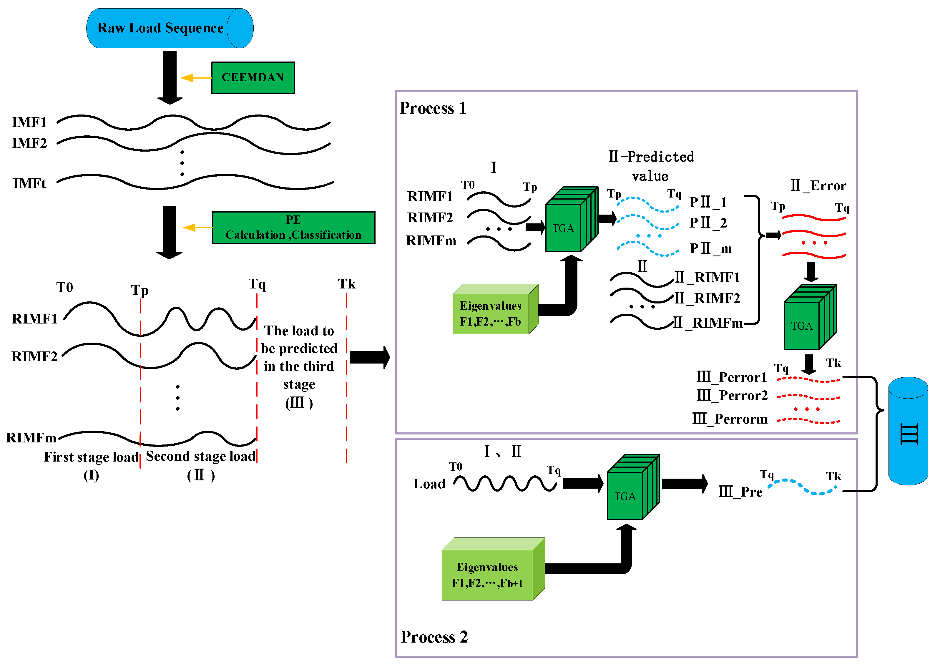
• Part 1 (green region): The original power load sequence is divided into three stages. Firstly, the data of the first and second stages are decomposed using the CEEMDAN algorithm into several intrinsic mode functions (IMFs). The permutation entropy values are calculated for each IMF, and the IMFs with similar permutation entropy values and similar trends of decomposition curves are grouped together. The grouped IMFs are summed to obtain several recombined IMFs. The TCN, GRU, and attention mechanism form the TGA model, which is used to process and predict the load sequence. Next, the first-stage load sequence and factors such as weather and economy are input into the TGA model for training in order to predict the load values of the second stage. The difference between the real values and the predicted values of the second stage is calculated as the error sequence. Finally, the error sequence is input into the pre-trained TGA model in order to predict the error values of the third stage.
• Part 2 (yellow region): Firstly, the first- and second-stage load sequences are decomposed using the seasonal and trend decomposition using Loess (STL) algorithm to obtain their trend features. Then, the average load sequence of the historical four years during the same period as the third stage is calculated. The STL algorithm is applied to the historical load sequence of the third stage using the same procedure to obtain its trend features. Next, the trend feature sequences are merged with the original weather and economic factors in order to form a new feature matrix. Finally, the first- and second-stage load data, along with the feature matrix, are input into the TGA model in order to predict the load sequence of the third stage.
• Part 3 (blue region): The predicted error sequence of the third stage is combined with the predicted load sequence of the third stage to obtain the final target sequence.

3. Applied Methodologies

3.1. Trend Feature Extraction

The factors influencing power load include weather, economy, time, etc. The load in spring and autumn is relatively close to that in summer and winter. This study not only considers climatic factors, but also innovatively extracts features from historical load data in the same time period as an additional influencing factor combined with climate factors for reconstruction into a new and more comprehensive feature, which is then used as an input for load forecasting models.

Time series generally consist of trends, seasonal variations, and residuals. A three-stage approach is employed in this paper to predict the error term in the third stage, making it approximate to the randomness or irregular fluctuations caused by accidental factors. Climate factors are used as feature values to approximate the impact of seasonal variations. Trend term extraction from historical load data in the same period can provide some trend guidance for the prediction model. The trend feature extraction of the historical load sequence is as follows:

Assume that there are n groups of time series of length m in the same period: $X_1,X_2,X_3,\dots ,X_n$, where $X_i=\left(x_{i1},x_{i2},x_{i2},\dots ,x_{im}\right)$, the matrix form is as follows:

$$X_{n\times m}=\left(\begin{array}{l}{x}_{11},x_{12},x_{13},\dots ,x_{1m}\\ x_{21},x_{22},x_{23},\dots ,x_{2m}\\ \dots \dots \\ x_{n1},x_{n2},x_{n3},\dots ,x_{nm}\end{array}\right)$$

$$\stackrel{-}{x}=\frac{{\displaystyle \sum _{i=1}^n{x}_i}}{n}$$

(1)

Put each row in X_n×m into Equation (1) to receive $X_{\mathrm{mean}}=\left(\stackrel{-}{x_1,}\stackrel{-}{x_2,}\stackrel{-}{x_3,}\stackrel{-}{\dots ,x_m}\right)$. Among them, X_mean is the averaged sequence of the X_n×m sequence.

X_mean is decomposed into trend items, periodic items, and irregular remainder items by the STL time series [5,42] according to the principle of the additive model [43] as follows:

$$X_v=T_v+S_v+R_v$$

(2)

where X_v is the X_mean value at v moment and T_v, S_v, and R_v are the trend value, cycle value, and residual value at that moment, respectively.

The X_mean sequence data are fitted using locally weighted regression (Loess) [44]. Before fitting, the regression order d, the sequence length q, and the weight function should be determined. Assuming that the positive integer is q ≤ t (the value of t represents the number of subsequences of the sequence), the q points closest to x are selected as the regression data, and the weight is calculated using the distance between each x_i and x. The weight calculation method is as follows:

$$\begin{array}{c}{W}_{\left(u\right)}=\{\begin{array}{c}\hfill {\left(1-u^3\right)}^3\hspace{1em}\hspace{1em}\hspace{1em}\left(0\le u\le 1\right)\hfill \\ \hfill 0\hspace{1em}\hspace{1em}\hspace{1em}\hspace{1em}\hspace{1em} \left(u>1\right)\hfill \end{array}\\ u=\frac{\left|x_i-x\right|}{{\lambda }_q\left(x\right)}\end{array}$$

(3)

where W_(u) represents the weight of the qth point near x. When q is greater than t, λ_t(x) denotes the maximum removal between x_i and x in this case.

$${\lambda }_q\left(x\right)={\lambda }_t\left(x\right)\frac{q}{t}$$

(4)

STL decomposition is divided into an inner loop and an outer loop. Let $T_{\mathrm{v}}^{\left(k\right)}$ and $S_{\mathrm{v}}^{\left(k\right)}$ be the trend and periodicity values at the end of the (k − 1)th inner loop, respectively. Set $T_{\mathrm{v}}^{\left(1\right)}=0$, the number of inner loop iterations as z_(i), the number of robust outer loop iterations as z_(o), the number of data samples in each cycle as z_(p), the smoothing parameter for separating the periodicity component as z_(s), the smoothing parameter for the low-pass filter as z_(l), and the trend smoothing parameter as z_(r). Refer to the following information for more detailed information on these parameters [43].

Inner loop:

• Subtract the previous trend value from the time series value x_v at time V: $X_{\mathrm{v}}-T_v^{\left(k\right)}$;
• Fit the subsequence using Loess and extend it forward and backward by one period, denoted as $C_v^{\left(k+1\right)}$;
• The composed signal $C_v^{\left(k+1\right)}$, which consists of z_(p) groups, should undergo the application of a low-pass filter, and perform a slide smoothing of length z_(p), z_(p), and 3 sequentially. Perform Loess regression with d = 1 and q = z_(l), resulting in $L_v^{\left(k+1\right)}$;
• Detrend: $S_v^{\left(k+1\right)}=C_v^{\left(k+1\right)}-L_v^{\left(k+1\right)}$;
• Decycle: $T_v^{\prime }=X_v-S_v^{\left(k+1\right)}$;
• Perform $T_v^{\prime }$ regressions to obtain $T_v^{\left(k+1\right)}$.

Next, in the outer loop, the deviation between the actual value and the estimated value is calculated at point i: $B_i=\left|g\left(x_i\right)-x_i\right|$.

$$W\left(o\right)=\{\begin{array}{cc}{\left(1-o^2\right)}^2& \left(0\le o\le 1\right)\\ 0& \left(o<0, o>1\right)\end{array}$$

(5)

Equation (5) calculates the robustness weight at x_i point, where the larger the value of B_i, the smaller the weight, where W_(o) represents the robustness weight, $o=\left|\frac{B_i}{h}\right|$, h = 6 × median(B_i).

After the inner and outer loops, the trend component T_v is obtained and denoted as X_trend.

$$x_{tren{d}_{imputed,j}}=\{\begin{array}{ll}{x}_{trend,j}& x_{trend,j}\ne NaN\\ \frac{{\displaystyle \sum _{i=1}^n{x}_{i,j}}}{n}& x_{trend,j}=NaN\end{array}$$

(6)

Equation (6) is used to handle the outliers in X_trend. In the equation, NaN denotes the outlier. When the j-th value is an outlier in the first and second stages, it is replaced by the actual value, while in the third stage, it is replaced by the historical average value ${\stackrel{-}{x}}_j$.

Finally, the processed X_trend is normalized to obtain X_normal, which represents the desired trend feature. The obtained data are merged with the climate factors to create a new feature dataset with an additional dimension.

$$x_{normal,i,j}=\frac{x_{trend,j}-\min \left(X_{trend}\right)}{\max \left(X_{trend}\right)-\min \left(X_{trend}\right)}$$

(7)

According to the above information, the summary of extracting historical load trend features can be divided into six steps. Firstly, the historical four-year power load data corresponding to the target sequence time period are added, and the average value is obtained. Secondly, the STL decomposition is performed on the averaged sequence obtained in the first step to extract the trend component. Thirdly, the abnormal values in the trend component obtained in the second step are replaced by the average value. Fourthly, the processed sequence is normalized. Fifthly, if the first- and second-stage sequences are extracted directly, the first step is skipped. Lastly, the obtained sequence is merged with the climate factor features to reconstruct a new feature dataset with an additional dimension.

3.2. CEEMDAN Algorithm

The power load sequence exhibits multi-frequency characteristics, where high-frequency components represent small-scale variations of the load curve over short periods, while low-frequency components represent smooth changes. CEEMDAN is employed for the investigation of internal variation patterns within the load sequence. White noise is introduced into CEEMDAN with the opposite sign to the original load sequence to avoid endpoint effects and mode mixing, making it more advantageous for time series decomposition [45].

Let L_(t) represent the original power load sequence, the i-th intrinsic mode function component, denoted as $\overline{C_i\left(t\right)}$, obtained by CEEMDAN decomposition, V^j is the added Gaussian white noise signal, where j denotes the number of noise additions and ε is the noise standard deviation. The decomposition process is as follows:

• The L_(t), augmented with noise, is decomposed by EMD, yielding the first-order intrinsic mode function C₁: $EMD\left(L_{\left(t\right)}+{\left(-1\right)}^q\epsilon V^j\left(t\right)\right)=C_1^j\left(t\right)+r^j$, where q = 1, 2;
• The first intrinsic component $\overline{C_1\left(t\right)}$ is obtained by the mean value of all of the modal components taken together: $\overline{C_1\left(t\right)}=\frac{1}{N}{\displaystyle \sum _{j=1}^N{C}_1^j}\left(t\right)$;
• The calculation of residuals: $r_1\left(t\right)=L_{\left(t\right)}-\overline{C_1\left(t\right)}$;
• The r₁(t) signal is subjected to EMD decomposition after the addition of positively and negatively paired white noise, resulting in the first-order modal component D₁, and thus obtaining the second intrinsic mode component: $\overline{C_2\left(t\right)}=\frac{1}{N}{\displaystyle \sum _{j=1}^N{D}_1^j}\left(t\right)$;
• The second residual is computed: $r_2\left(t\right)=r_1\left(t\right)-\overline{C_2\left(t\right)}$;
• By repeating these steps, a total of K intrinsic mode components is obtained, where the power load data are: $L_{\left(t\right)}={\displaystyle \sum _{k=1}^K\overline{C_k\left(t\right)}}+r_k\left(t\right)$.

CEEMDAN decomposition adds white noise with opposite signs, which is independent and identically distributed. After averaging the ensemble of components, the auxiliary white noise can be greatly reduced. Therefore, the load sequence is still the signal itself after decomposition, effectively solving the problems of white noise residue, reconstruction error, and completeness missing in EEMD decomposition, and reducing experimental errors.

3.3. Principle of TGA Model

Lea et al. applied temporal convolutional networks to time series forecasting [46]. TCN is capable of extracting the temporal relationships in data in parallel and builds upon convolutional neural networks (CNN) by incorporating causal convolutions, dilated convolutions, and residual blocks.

Causal convolution ensures that the data passes through in one direction, and the data of the next layer depends on the values at the same time in the preceding layer and in earlier stages, therefore, causal convolution does not consider future values. If it is necessary to learn more data from the past, more hidden layers could be added at the front.

$${\left(F\times \mathrm{d}X\right)}_{\left(x_t\right)}={\displaystyle \sum _k^K{f}_k}{x}_t-\left(K-k\right)d$$

(8)

Equation (8) is used to calculate the dilation factor. Dilated convolution allows convolution to skip part of the input to achieve an expanded receptive field, and the range of convolution is controlled by the dilation factor, where the number of layers is represented by d, k is the kernel size, F is the filter with F = (f₁, f₂, …, f_k), and X is the time series.

Figure 2 shows the dilated causal convolution principle. With an increase in level, the effective window size of dilated convolution expands exponentially in accordance with the number of layers, enabling the convolutional network to achieve a larger receptive field in general.

Figure 3 shows the principle of the GRU cell structure. The internal structure bears similarities to LSTM. However, GRU is characterized by the presence of only two gates, which reduces “gate control,” and also has relatively fewer parameters. Therefore, the GRU model reduces the computation time compared to LSTM [44], while being equally functional. When building models with multiple neural networks in parallel, the GRU model is preferable.

The reset gate (r_t) and the update gate (z_t) are two key components of GRU. σ corresponds to the sigmoid function, tanh corresponds to the tanh function, and 1- represents the forward propagation data with a size of 1−z_t. The pink circle with a dot inside represents the dot product operation between the matrices, and the plus sign represents the matrix addition operation. The hidden layer output is denoted as h_t, and the data input is represented by x_t, where W_r and W_z are weight matrices.

$$z_t=\sigma \left(W_z\cdot \left[h_{t-1},x_t\right]\right)$$

(9)

$$r_t=\sigma \left(W_r\cdot \left[h_{t-1},x_t\right]\right)$$

(10)

$${\tilde{h}}_t=\tanh \left(W\cdot \left[r_t\times h_{t-1},x_t\right]\right)$$

(11)

$$h_t=\left(1-z_t\right)\times h_{t-1}+z_t\times {\tilde{h}}_t$$

(12)

Figure 4 shows the principle of the attention mechanism. It can compute the contribution rate of the output data. The box part represents the calculation principle of the attention mechanism; h₁, h₂, …, h_n are the input data of the attention mechanism, which are the output data of the GRU layer; α₁, α₂, …, α_n are the allocated weight values of the data; and y is the final result.

Equation (13) represents the attention mechanism as follows, where * means weighted operation:

$$Attention\left(Query,Source\right)={\displaystyle \sum _{i=1}^{L_x}Similarity\left(Query,Ke{y}_i\right)}\ast Valu{e}_i$$

(13)

In short-term load forecasting, since the predicted time steps are short, it is necessary to mine historical information and preserve most of the information at each step. The causality between the TCN convolutional layers means that there will be no “missing” historical information or future data that can extract information from the historical load sequence [47]. The extracted information features are input into the GRU to enable it to better study the correlation and regularity of the information. The excellent structural design of GRU enables the maximum preservation of features for sequential learning and propagation at each time step. When the important feature information is transmitted in GRU, in order to avoid the decrease in the importance of information in each level caused by a long time period and long sequence, based on this foundation, the present study introduces an attention mechanism after the output layer of GRU to perform weighted processing of the important features outputted by GRU, thereby preserving important information and improving prediction accuracy.

Figure 5 shows the principle of the TGA model. It is used to accomplish important load sequence processing tasks, such as data mining, information storage and transmission, and feature learning. The load to be predicted, the error, and the influencing factors are first subjected to feature selection through the TCN layer, and then the selected features are transformed through a connection layer for dimensionality reduction. The GRU and attention layers receive the input of data features for the purpose of learning and weighting. Finally, the output layer outputs the predicted value.

• Input Layer: Merge and normalize the power load sequence $x={\left[x_1,x_2,x_3\dots x_n\right]}^T$ and feature sequence $F=\left[f_1,f_2,f_3\dots f_m\right]$ to obtain the sequence $X=\left[X_1,X_2,X_3\dots X_n\right]$ as input.
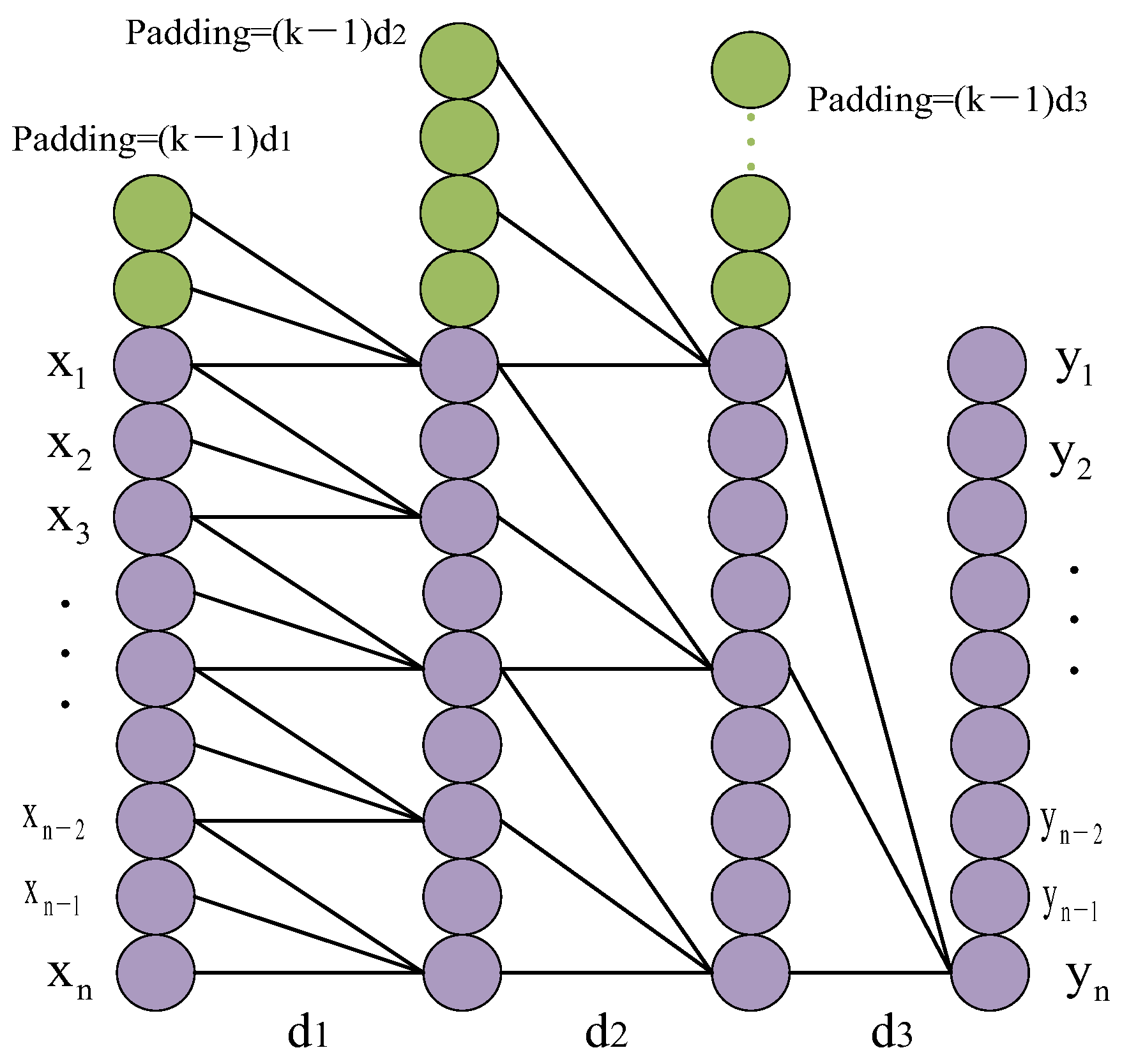
• TCN Layer: Use a single layer of residual units. Configure a single residual unit with two convolutional units and one non-linear mapping layer. To reduce dimensionality, add a 1 × 1 convolution layer into the residual mapping layer. The operation of one-dimensional dilated causal convolution is expressed as follows, where $C_t={[c_1,c_2\dots c_i]}^T$ is the output result of the TCN layer:

  $$F\left(s\right)={\displaystyle \sum _{i=0}^{k-1}f\left(i\right)}{x}_{s-di}$$

  (14)

  where x is the input sequence, f is the filter, d is the dilation factor, k is the kernel size, and s − d_i ensures that only past inputs are convolved.
• GRU Layer: Feed the output C_t from the TCN layer into a single-layer GRU model, which learns the extracted feature information. The output of the kth step of the GRU is denoted as h_k, which is obtained using Equation (15):

  $$h_k=GRU\left(c_{k-1},c_k\right),k\in \left[1,i\right]$$

  (15)
• Attention Layer: Equations (16)–(18) represent the calculation process of weight coefficients. Compute the probabilities associated with various feature information by applying the weight allocation rules and derive the weight parameter matrix through iterative updating.

  $$e_k=u\tanh \left(w{h}_k+b\right)$$

  (16)

  $$a_k=\frac{\exp \left(e_k\right)}{{\displaystyle \sum _{j=1}^k{e}_j}}$$

  (17)

  $$s_k={\displaystyle \sum _{k=1}^i{a}_k}{h}_k$$

  (18)

  where e_k represents the attention probability distribution value at time k; u and w are weight coefficients; and b is the bias coefficient. The output of the attention mechanism layer at time k is denoted as s_k.
• Output Layer: Equation (19) represents the predicted result of denormalization.

  $$y_k=Sigmoid\left(w_q{s}_k+b_q\right)$$

  (19)

  where y_k represents the predicted value at time step k; w_q is the weight matrix; and b_q is the bias.

3.4. Principle of Three-Stage Load Forecasting

Figure 6 shows the three-stage load forecasting process. The three stages refer to three different time periods. The historical power load sequence is divided into stage one and stage two, and the load sequence to be predicted is in stage three. The lower the stage number, the earlier the time period, assuming that there is an original power load sequence of $X=[x_1,x_2,x_3,\dots ,x_{n-1},x_n]$ in time periods T₀~T_q, which is decomposed into t intrinsic mode functions ${[\mathrm{IMF}}_1{,\mathrm{IMF}}_2,\dots {,\mathrm{IMF}}_{\mathrm{t}}]$ by CEEMDAN, each of length n. Next, the IMF series are classified based on a permutation entropy calculation, and the sum of the IMF values in each class is obtained to form m recombined IMFs ${[\mathrm{RIMF}}_1{,\mathrm{RIMF}}_2,\dots {,\mathrm{IMF}}_m]$, where m < t. The m components are divided into two time periods, where the initial time is T₀; the beginning of the second stage is T_p; the beginning of the third stage is T_q; and the end of the prediction stage is T_k. T_p to T_q and T_q to T_k have the same length. At this time, the subsequence of the T₀~T_p time period is $\left(\begin{array}{l}RIMF{1}_{T0},RIMF{1}_{T1},\dots ,RIMF{1}_{TP}\\ RIMF{2}_{T0},RIMF{2}_{T1},\dots ,RIMF{2}_{TP}\\ . . .\\ RIMF{\mathrm{m}}_{T0},RIMF{m}_{T1},\dots ,RIMF{m}_{TP}\end{array}\right)$, and the subsequence of the T_p~T_q time period is $\left(\begin{array}{l}RIMF{1}_{Tp},RIMF{1}_{T\left(p+1\right)},\dots ,RIMF{1}_{Tq}\\ RIMF{2}_{Tp},RIMF{2}_{T\left(p+1\right)},\dots ,RIMF{2}_{Tq}\\ . . .\\ RIMF{\mathrm{m}}_{Tp},RIMF{m}_{T\left(p+1\right)},\dots ,RIMF{m}_{Tq}\end{array}\right)$.

The preprocessed data sequence is divided into two processes for computation. The first process predicts the error sequence of the third stage and the second process predicts the load sequence of the third stage.

In Process 1, the feature value sequence of the first stage is mainly composed of five influencing factors in climate and economy, namely dry bulb temperature, relative humidity, and electricity price, as follows: $F=\left(\begin{array}{l}{f}_{11},f_{12},\dots ,f_{1n}\\ f_{21},f_{22},\dots ,f_{2n}\\ . . .\\ f_{51},f_{52},\dots ,f_{5n}\end{array}\right)$. In order to predict the component values in the time period T_p to T_q, each component of the time period T₀ to T_p is sequentially trained with feature F₁ and input into the model. The predicted component values for the time period T_p to T_q are denoted as P_{Ⅱ_IMF}. $P_{\mathrm{II}}\_IMF=\left(\begin{array}{l}{P}_{\mathrm{II}}\_1_{T\mathrm{p}},P_{\mathrm{II}}\_1_{T\left(\mathrm{p}+1\right)},\dots ,P_{\mathrm{II}}\_1_{Tq}\\ P_{\mathrm{II}}\_2_{T\mathrm{p}},P_{\mathrm{II}}\_2_{T\left(\mathrm{p}+1\right)},\dots ,P_{\mathrm{II}}\_2_{Tq}\\ \dots \\ P_{\mathrm{II}}\_m_{T\mathrm{p}},P_{\mathrm{II}}\_m_{T\left(\mathrm{p}+1\right)},\dots ,P_{\mathrm{II}}\_m_{Tq}\end{array}\right)$. The error matrix II_Error for the second stage is obtained by subtracting the predicted values of P_{II_IMF} from the actual values as follows: $\mathrm{II}\_Error=\left(\begin{array}{l}\mathrm{II}\_error{1}_{T\mathrm{p}},\mathrm{II}\_error{1}_{T\left(\mathrm{p}+1\right)},\dots ,\mathrm{II}\_error{1}_{Tq}\\ \mathrm{II}\_error{2}_{T\mathrm{p}},\mathrm{II}\_error{2}_{T\left(\mathrm{p}+1\right)},\dots ,\mathrm{II}\_error{2}_{Tq}\\ \dots \\ \mathrm{II}\_error{m}_{T\mathrm{p}},\mathrm{II}\_error{m}_{T\left(\mathrm{p}+1\right)},\dots ,\mathrm{II}\_error{m}_{Tq}\end{array}\right)$. Finally, the sequence of Ⅱ_Error is placed into the TGA model to predict the error values of each modal component in the third stage, denoted as Ⅲ_PError.

The three-stage load forecasting method decomposes the power load sequence into various sub-mode components, as it is beneficial to group together internal features with similar trends for classification processing. Simultaneously, subdividing and predicting the error sequence can reduce the prediction errors of the third stage. Moreover, the reconstructed feature values can enable the TGA model to learn the trend and seasonality of the historical sequences. In short, the three-stage load forecasting aims to predict the trend, seasonal, and residual items of the load sequence and strives to stratify the prediction to minimize the overall error of the target sequence.

3.5. Model Evaluation Indicators

This paper uses four model evaluation metrics, namely mean absolute error (MAE), coefficient of determination (R²), root mean squared error (RMSE), and mean absolute percentage error (MAPE), where y_i and $\widehat{y_i}$ represent the true and predicted values at the same time, and m is the number of elements in the power load sequence.

$$\mathrm{MAE}=\frac{1}{m}{\displaystyle \sum _{i=1}^m\left|\left(y_i-\widehat{y_i}\right)\right|}$$

(20)

$${\mathrm{R}}^2=1-\frac{{\displaystyle \sum _{i=1}^m{\left(y_i-\widehat{y_i}\right)}^2}}{{\displaystyle \sum _{i=1}^m{\left(y_i-\overline{y_i}\right)}^2}}$$

(21)

$$\mathrm{RMSE}=\sqrt{\frac{1}{m}{\displaystyle \sum _{i=1}^m{\left(y_i-\widehat{y_i}\right)}^2}}$$

(22)

$$\mathrm{MAPE}=\frac{1}{m}{\displaystyle \sum _{i=1}^m\left|\frac{y_i-\widehat{y_i}}{y_i}\right|}\times 100\%$$

(23)

4. Purpose of Experiment

The proposed theoretical method is validated using electricity load data from Australia and Quanzhou, China. A comparison is made between the decomposition and the reconstruction of the electricity load series using CEEMDAN and PE algorithms, as well as the non-decomposed case, to determine if it reduces volatility. The final prediction results curve and evaluation metrics are used to assess whether the proposed method improves the prediction accuracy and reduces fitting errors compared to other methods. The following sections are arranged as follows: Section 5.1 decomposes the first and second-stage load series of the Australian dataset; Section 5.2 extracts the trend features from the historical load series; Section 5.3 compares the prediction performance of the TGA model with other algorithmic models; Section 5.4 analyzes the differences between the use of decomposition algorithms and the non-use of decomposition algorithms; Section 5.5 presents the prediction of the target sequence and its result analysis; and Section 5.6 presents the experimental results and analysis of the Quanzhou dataset.

5. Results

5.1. Decomposition of Power Load Sequence

Section 5.1, Section 5.2,Section 5.3, Section 5.4 and Section 5.5 will be dedicated to validating the proposed theoretical method using the electricity load data from Australia. The dataset includes temperature, humidity, electricity price, and load data, as shown in

Table 1. Partial power load data and influencing factors in Australia.

Dry Bulb Temperature (°C)	Dew Point Temperature (°C)	Wet Bulb Temperature (°C)	Humidity	Electricity Price (AUD/GJ)	Load (MW)
24.5	19.7	21.4	75	21.33	8531.56
24.95	19.85	21.65	73.5	21.71	9068.78
25.4	20	21.9	72	22.6	9756.34
26.2	19.7	22	67.5	23.26	10,338.65
27	19.4	22.1	63	23.71	10,742.79
26.7	19.85	22.25	66	28.02	11,178.09
26.4	20.3	22.4	69	30.73	11,455.07
26.6	20.25	22.45	68	34.35	11,659.23
26.8	20.2	22.5	67	35.16	11,808.46
26.9	20.35	22.6	67.5	40.95	11,903.07
27	20.5	22.7	68	39.28	12,073.69
27.05	20.3	22.6	67	36.94	12,145.38
27.1	20.1	22.5	66	33.31	12,177.38
26.5	19.9	22.2	67.5	32.79	12,199.36
25.9	19.7	21.9	69	34.05	12,157.97

. Figure 7 shows the selected experimental data of 1800 points every half an hour from 6:00, 13 January 2010 to 18:00, 19 February 2010, in a certain region of Australia as the dataset, and Table 1 shows some of the data points. The dataset is divided into the first stage, i.e., the first time period, the second stage, and the third stage, in which the ratio is 4:1:1 and the third stage is the prediction stage.

Figure 8 shows the CEEMDAN decomposition of 1200 points from 6:00, 13 January 2010 to 5:30, 13 February 2010. Eight sub-feature modal components were obtained from the decomposition. From the figure, it is evident that the change trends of IMF1 and IMF2 are relatively compact. Specifically, the changes in peak values are very similar; the trend of IMF3 is basically consistent with the original sequence; and IMF4, IMF5, IMF6, IMF7, and IMF8 have relatively gentle trends, with relatively few extreme points.

Figure 9 shows the distribution of permutation entropy values of the sub-mode components, which further classifies the sub-mode components by judging their complexity. Here, m represents the embedding dimension and t represents the delay step size. From the figure, regardless of the selection of m or t, it is evident that the values of IMF1 and IMF2 are greater than 0.5, while the values of IMF3 to IMF8 are relatively small and tend to be flat. This indicates that the complexity of IMF1 and IMF2 is high and similar, while the complexity of IMF3 to IMF8 is low and similar.

Figure 10 shows the reconstructed sub-components after the analysis of trend and permutation entropy values. IMF1 and IMF2 were combined into a new sequence due to their similar and complex trend patterns. IMF3, which is similar to the original curve, was classified as a separate component. IMF4 to IMF8, with a relatively flat trend and low complexity, were grouped into another component. The reconstructed sub-sequences are denoted as RIMF, and there are a total of three groups.

Table 2. Correlation coefficients among the eigenmode components of the restructured power load sequence.

	RIMF1	RIMF2	RIMF3	Load
RIMF1	1	0.177	0.027	0.332
RIMF2	0.177	1	−0.050	0.863
RIMF3	0.027	−0.050	1	0.434
Load	0.332	0.863	0.434	1

shows the correlation coefficients among the three reconstructed sub-sequences. It can be observed from the table that the three reconstructed sub-sequences have a high correlation with the original power load, while the correlation among the three sub-sequences is relatively low, indicating that the classification and reconstruction results are satisfactory.

5.2. Extracting Historical Data Features

In order to extract the features of the historical load data, the average trend component of the third stage for the first four years is extracted. This paper predicts a range of 300 points from 6:00 on 7 February 2010 to 12:00 on 13 February 2010.

Figure 11 shows the power load curves for the same time period from 2006 to 2009. It can be seen that the load sequence has a period of 48 points for 24 h. Although the peak values of the load in these four years are different, the time points of the peaks are quite similar, and the trend of the curve changes is very similar. Therefore, the average trend of these four years is extracted as the feature value input for the year 2010 to facilitate the learning of the prediction model. First, the average load sequence for a period of four years is calculated; second, the trend item of the mean sequence and the first- and second-stage trend items are extracted using the STL method according to the steps in Section 3.1. Since the trend item has outliers, the mean value replacement is used for the trend item of the third stage of the mean sequence, the real value replacement is used for the first and second stages, and, finally, normalization is performed.

Figure 12 shows the complete trend sequence, and it can be observed that the overall trend of the trend curve is similar to that of the historical load trend. At the peak, the extreme points are mainly distributed in the dense areas of the historical curve. Overall, the trend curve represents the trend development of multiple historical load curves.

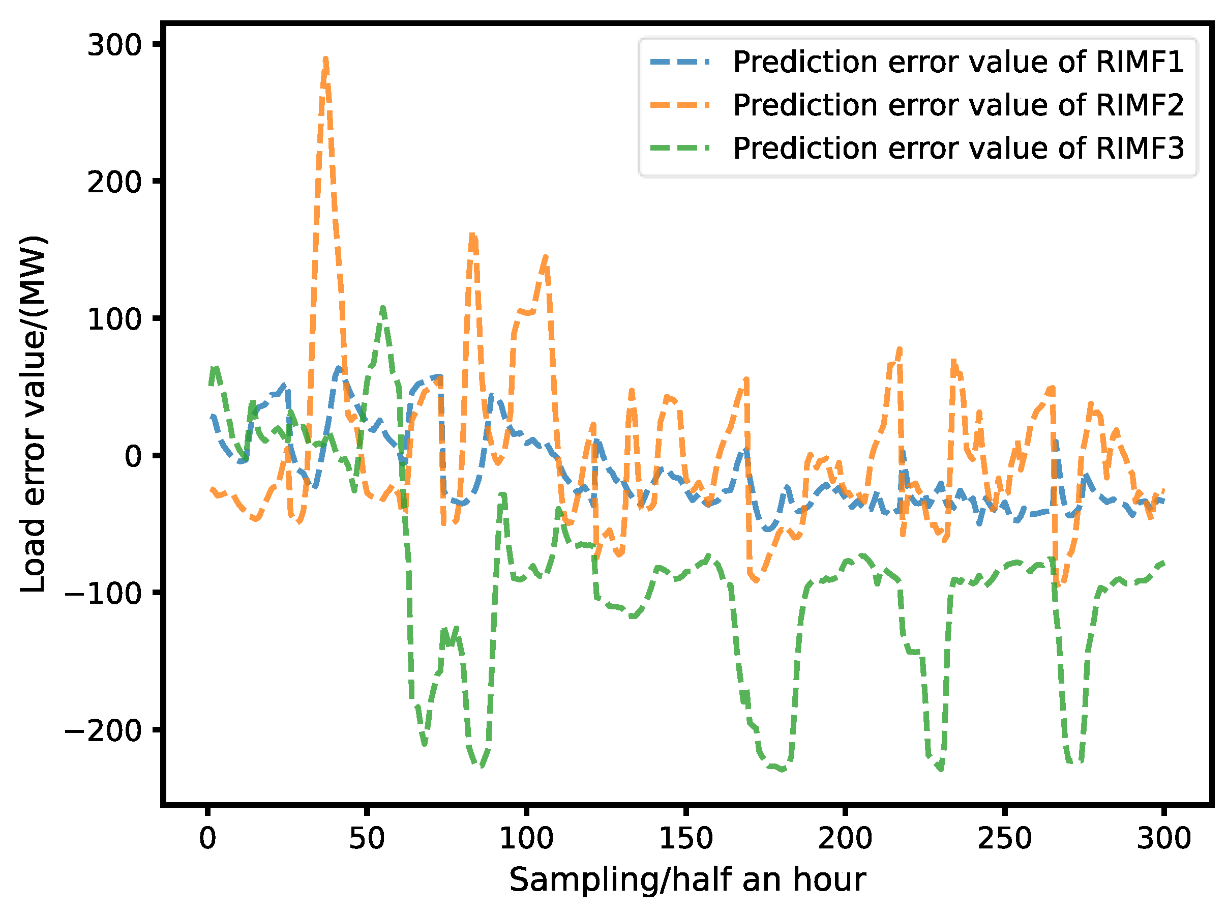
5.3. Model Prediction Results Analysis

Figure 13 shows a comparison of the TGA model, the GRU neural network combination model, and the machine learning model. To evaluate the short-term prediction capability of the TGA model, this paper compares it with the machine learning models Adaboost, Random Forest (RF), and neural network GRU, as well as the combination model of TCN and GRU. The training sample starts at 6:00 on 13 January 2010, and the prediction period consists of 300 sample points in the second stage, with a sampling interval of 30 min. The curve fitting of Adaboost and Random Forest is the worst compared to the true values; however, they both describe the trend of the true values, with Random Forest showing sudden peak mutations in the range of the 170th and 220th predicted points, which the other models did not experience, indicating that the Random Forest algorithm is less stable. The curve trend effect of the GRU, TCN-GRU, and TGA model fitting is better; however, the TGA model gradually surpasses the other two models in terms of accuracy after the 50th predicted point, indicating that the TGA algorithm has the highest fitting degree and prediction accuracy.

Figure 14 shows the R², RMSE, MAPE, and MAE values of the five models. According to the figure, it is evident that the Adaboost and RF models have similar fit indicators; however, the RF model has lower RMSE and MAE values than the Adaboost model, indicating that the Adaboost model has a lower accuracy than the RF model. The GRU model has an RMSE of 263.024 MW, MAE of 216.783 MW, MAPE of 2.36%, and R² of 0.903. The TCN-GRU model has an RMSE of 242.381 MW, MAE of 185.41 MW, MAPE of 1.95%, and R² of 0.958. The TGA model has an RMSE of 190.938 MW, MAE of 156.678 MW, MAPE of 1.72%, and R² of 0.964. The fit indicators of the TCN-GRU and TGA models are significantly better than those of the others. Although the R² values of the TCN-GRU and TGA models are basically the same, the other three values of the TGA model are less than that of the TCN-GRU model. In conclusion, using the data in this study, the TGA model has better fit and lower error indicators than the Adaboost, RF, GRU, and TCN-GRU models.

Figure 15 shows the TGA model that was used to predict the results of RIMF1, RIMF2, and RIMF3 in the second stage, and

Table 3. Correlation coefficients among the eigenmode components of the restructured power load sequence.

	MAE/(MW)	R2	RMSE/(MW)	MAPE
RIMF1	100.126	0.870	133.224	260.420
RIMF2	127.304	0.978	174.986	22.544
RIMF3	47.520	0.981	63.799	6.520

shows the prediction indicators for each sub-mode component. As shown in the figure, the curve-fitting effect of RIMF1 to RIMF3 gradually improves. The data in the prediction indicator table show that R² increases in order from RIMF1 to RIMF3, while MAE, RMSE, and MAPE gradually decrease from RIMF1 to RIMF3. This is because the variation pattern of the RIMF1 curve is poor, and the model does not perform well in learning, while the RIMF3 curve has a relatively simple change pattern, and the model can extract important information during learning, leading to higher prediction accuracy.

Figure 16 shows the prediction errors for the second-stage modal components. The error values of RIMF1 and RIMF3 are relatively small, fluctuating around the 0 axis within a range of approximately −200 MW to 200 MW. However, at the 1st and 250th points, the absolute error values of RIMF1 and RIMF3 exceed 200 MW. The error range of RIMF2 is approximately −400 MW to 400 MW, and it exceeds 400 MW near the 250th point. Overall, the error values of the second-stage sub-feature modal components have relatively small fluctuations, which suggests that they can be used as inputs to predict the modal component errors of the third stage using the TGA model.

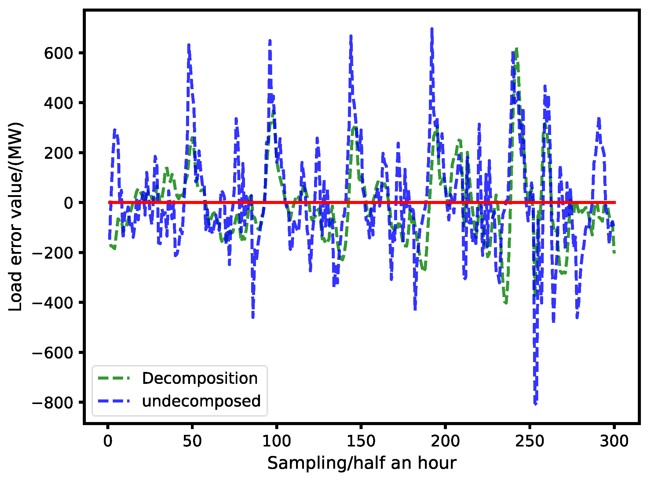
5.4. Decomposed and Undecomposed Results

Figure 17 shows the prediction error using CEEMDAN decomposition, classification, and unused results. When comparing the error sequence obtained in the decomposed case with that obtained in the undecomposed case, it can be observed that the decomposed error values fluctuate within the range of the zero-axis of the red line and occasionally experience sudden changes, while the undecomposed error values exhibit large ups and downs, with many points deviating from the zero-axis.

Table 4. The sum of the absolute values of the errors, the average value of the errors, and the maximum value of the errors.

	Sum of Absolute Values (MW)	Average Value (MW)	Maximum Value (MW)
Decomposition	33611.9	112.0	623.6
Undecomposed	46996.2	156.7	810.0

shows the sum of the absolute errors, mean error value, and maximum error. The sum, mean, and maximum absolute errors of the decomposed errors using CEEMDAN and PE classification are all smaller than those of the undecomposed errors. Therefore, it can be concluded that the sub-features of the sequence have been separated using the CEEMDAN decomposition and PE classification, and targeted prediction has effectively reduced the prediction error.

Figure 18 shows the prediction results of the target sequence using decomposition and non-decomposition, while

Table 5. Predictive evaluation indicators values under decomposed and undecomposed cases.

	MAE/(MW)	R2	RMSE/(MW)	MAPE
Decomposition	103.62	0.976	127.15	1.157
Undecomposed	109.75	0.970	157.313	1.307

presents the evaluation indicator values for both cases. The results from the figure and table indicate that, under the scenario of decomposition and reconstruction, although the values of MAE and R² are slightly smaller compared to the non-decomposition case, RMSE and MAPE are reduced by 19.17% and 11.48%, respectively.

In summary, regardless of the analysis perspective based on the sum of absolute errors, average error, or maximum absolute error, as well as the analysis from the perspective of the final predicted target sequence, it can be concluded that the adoption of CEEMDAN decomposition and permutation entropy reconstruction significantly reduces the prediction errors and improves the prediction accuracy. Therefore, the utilization of decomposition is an effective method for reducing the volatility of load sequences.

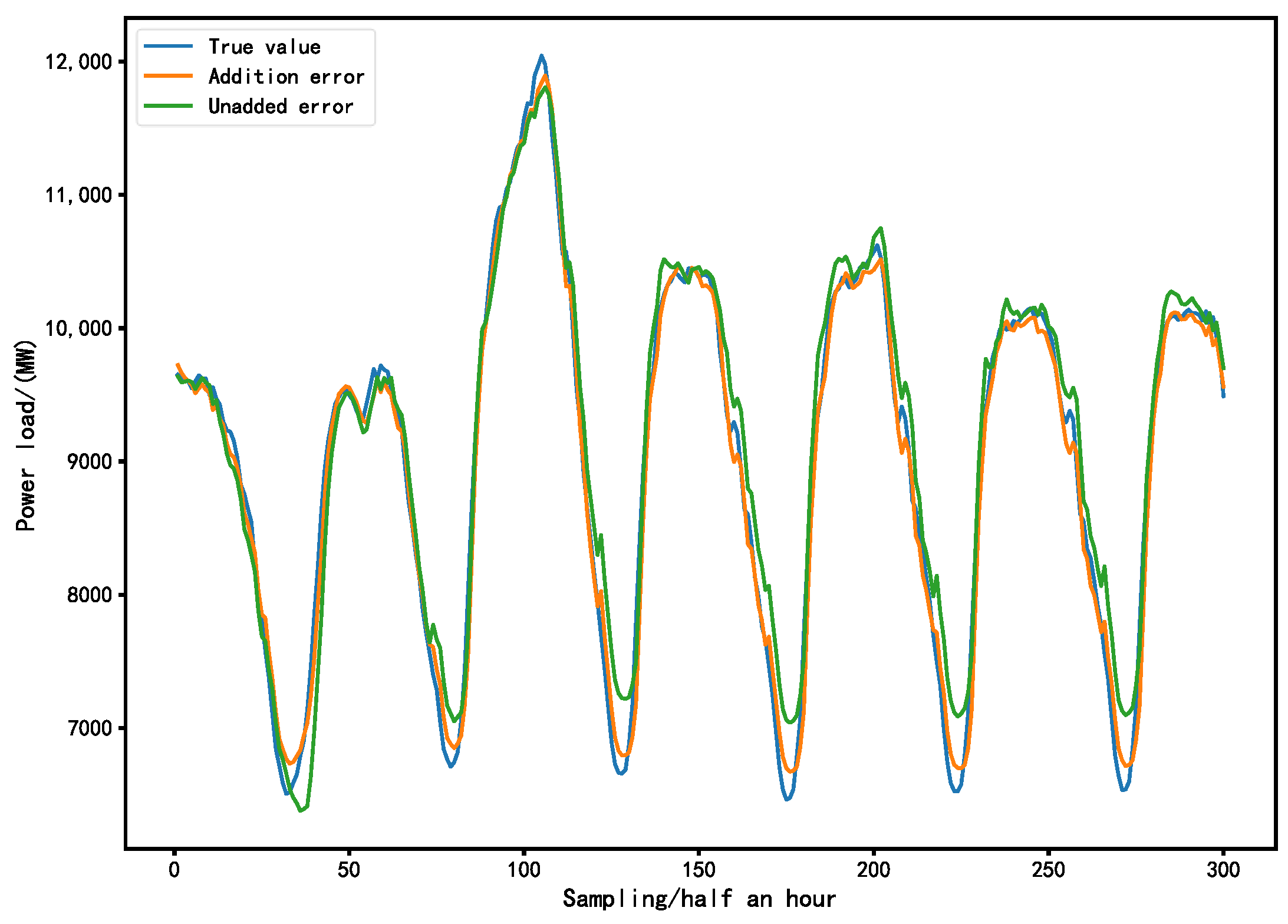
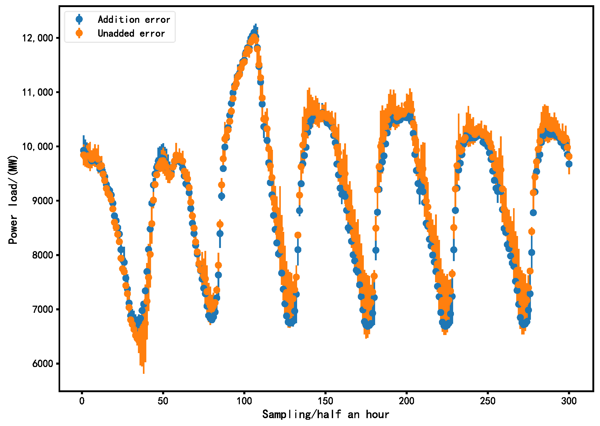
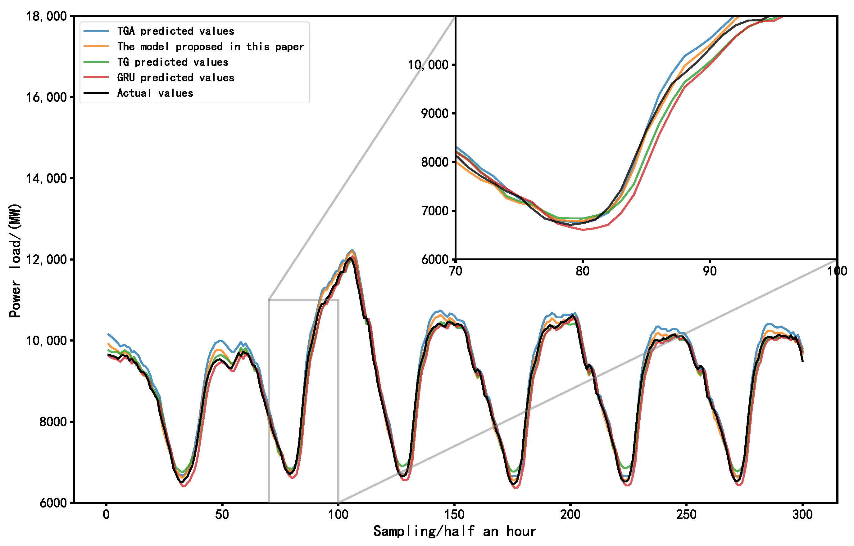
5.5. Target Sequence Prediction

To predict the third segment of power load, the first and second segment load values are used as a training set, with a time range from 5:30 on 13 January 2010 to 12:00 on 13 February 2010. One data point is taken every half an hour, resulting in 1500 data points. The prediction is made for the time period from 12:00 on 13 February 2010 to 17:30 on 19 February 2010, with a total of 300 data points. The influencing factors have been augmented with the addition of reconstructed feature values.

Figure 19 shows the prediction results of the third stage, obtained by training the error values of each group of RIMF1 and RIMF3 in the second stage using the TGA model. From the figure, it can be observed that the three predicted error sequences mainly fluctuate between −200 and 100 MW, with a few points fluctuating between 100 and 300 MW.

Figure 20 shows the simulation of 300 data points in the third stage using the TGA algorithm. The simulation is conducted with error addition, and the results are compared against the truth. From the curves, it can be observed that the prediction curve without added errors deviates significantly from the truth curve, especially at extreme points. In contrast, the fitting effect of the curve with added errors is noticeably superior to the one without added errors.

Figure 21 shows an error bar graph obtained by taking the difference between the true values and each sample point with and without added errors. The longer the vertical line, the greater the data variation or bias. It is evident that the vertical lines of points without added errors are longer than those with added errors. Therefore, it can be concluded that predicting the errors of the third-stage load by the errors predicted in the second stage has improved the prediction accuracy.

Figure 22 shows a comparison between the target sequence obtained by adding the predicted errors to the predicted stage-three load sequence and the sequences predicted by the GRU, TCN-GRU, and TCN-GRU-Attention models. The predicted points in the range of samples 70 to 100 are zoomed in on the upper right sub-figure, from which it can be seen that the predicted curve of the three-stage load prediction method proposed in this paper is closest to the trend of the actual value curve.

Table 6. The evaluation metrics for the GRU, TCN-GRU, TGA models without error value and three-stage load prediction model based on CEEMDAN-TGA.

	MAE/(MW)	R2	RMSE/(MW)	MAPE
Three-stage load prediction based on the CEEMDAN-TGA	95.581	0.982	125.23	1.099
TCN-GRU-Attention	106.433	0.971	130.17	1.187
TCN-GRU	129.001	0.965	167.58	1.534
GRU	167.001	0.921	233.492	1.997

shows the evaluation indicators of the different models. According to the data in the table, the MAE of the TGA model is 106.433 MW, the R² is 0.971, the RMSE is 130.17 MW, and the MAPE is 1.187; the MAE of the TG model is 129.0 MW, the R² is 0.965, the RMSE is 167.58 MW, and the MAPE is 1.534; the MAE of the GRU model is 167.0 MW, the R² is 0.921, the RMSE is 233.492 MW, and the MAPE is 1.997. The MAE, RMSE, and MAPE values of the three-stage load forecasting model are reduced by 10.19%, 25.9%, and 42.77%, respectively, compared to the TGA, TG, and GRU models. The RMSE is reduced by 3.8%, 25.27%, and 46.37%. The MAPE is reduced by 7.4%, 28.36%, and 45.0%.

Based on the data in the table, the following can be concluded:

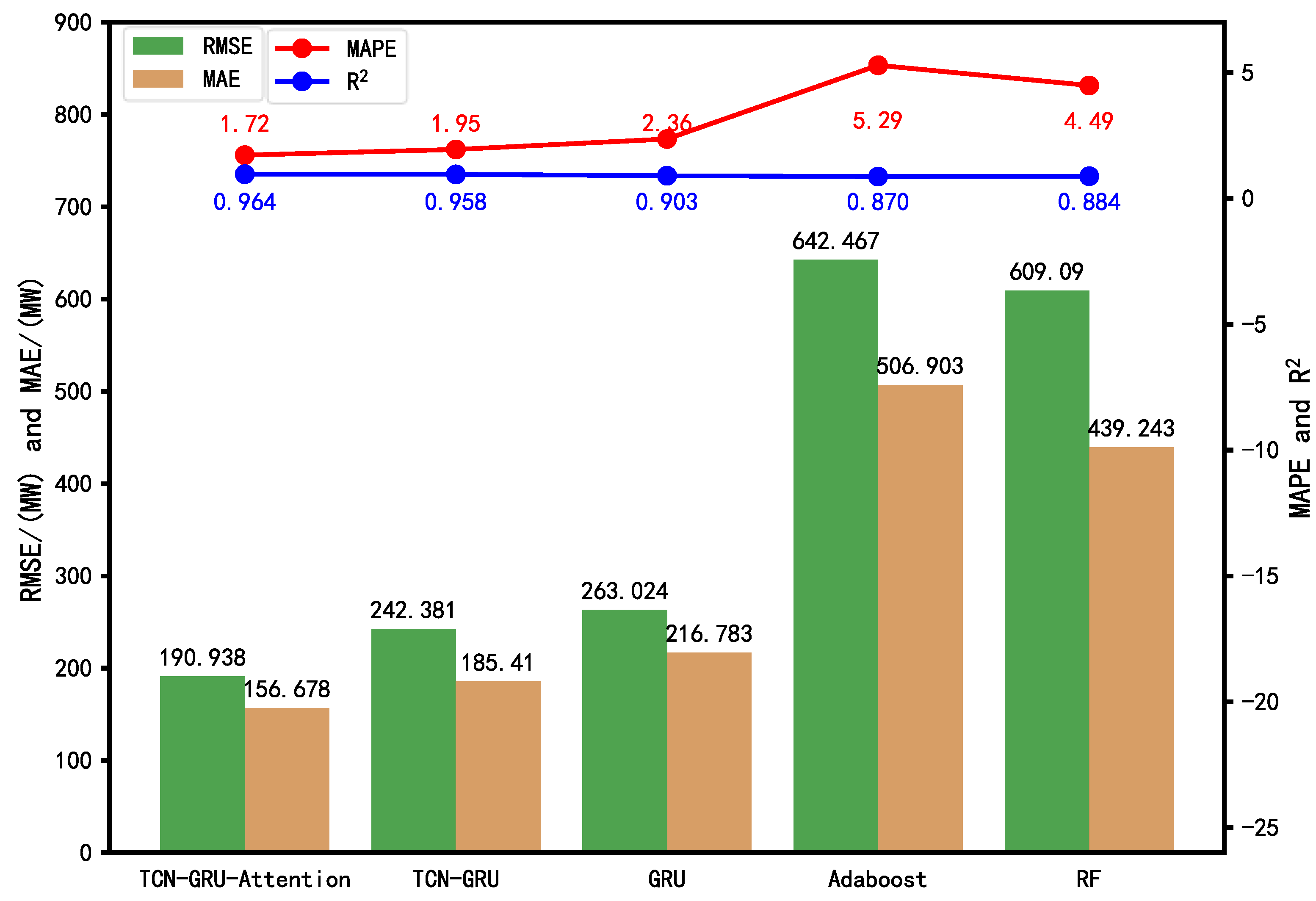
• The TCN-GRU model shows a decrease of 22.75% in MAE, 28.2% in RMSE, and 23.18% in MAPE compared to the GRU model, while the R² value increases by 4.78%. These data results indicate that combining the one-dimensional feature capability of the temporal convolutional network (TCN) with GRU improves the accuracy compared to using GRU alone;
• The TCN-GRU-Attention model demonstrates a decrease of 17.5% in MAE, 22.3% in RMSE, and 22.6% in MAPE compared to the TCN-GRU model, while the R² value increases to 0.971. These data results suggest that incorporating the attention mechanism into the TCN-GRU model can alleviate the progressive decrease in information importance and assign higher weights to important feature information outputs by GRU, thereby improving the prediction accuracy;
• The three-stage load prediction based on the CEEMDAN-TGA model proposed in this paper exhibits the lowest MAE, RMSE, and MAPE compared to the TGA, TG, and GRU models, with an R² value of 0.982. This indicates that the combination of CEEMDAN decomposition and permutation entropy-based recombination of sub-modal features performs well in reducing the volatility of load sequences. Additionally, extracting historical trend features and employing a three-stage data processing approach reduces model errors and enhances the prediction accuracy.

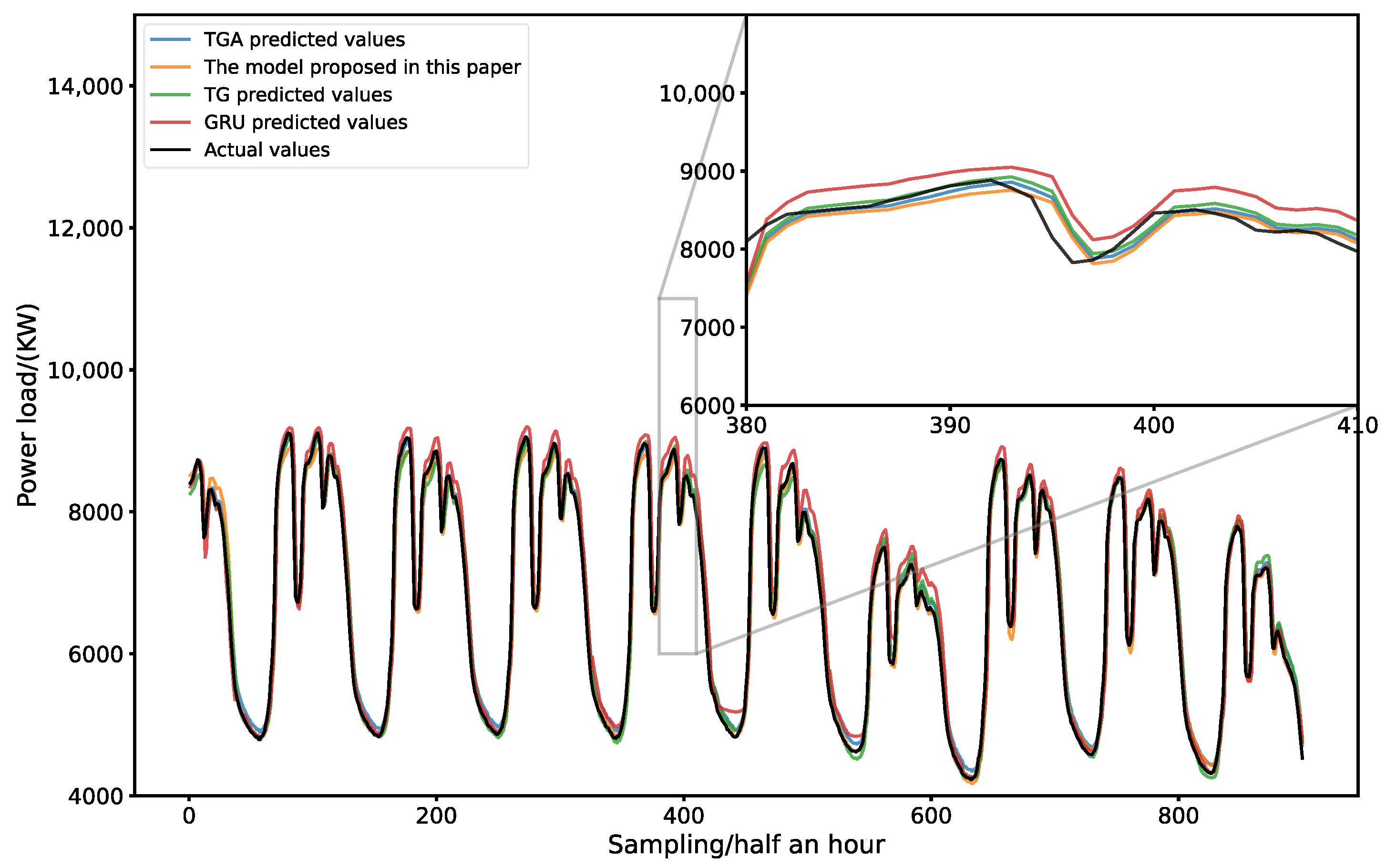
5.6. Data Verification in Quanzhou

This section employs electricity load data from Quanzhou, Fujian Province, China, to validate the aforementioned theoretical method.

Table 7. Partial power load data and influencing factors in Quanzhou, Fujian.

Maximum Temperature (°C)	Minimum Temperature (°C)	Average Temperature (°C)	Humidity	Precipitation	Load (KW)
15.1	11.2	12.1	87	0.5	2938.256
11.9	9.1	10.8	93	15.4	3221.17
9.2	6.4	7.4	69	2.9	3264.545
7.4	4.8	5.9	56	0	3880.76
6.2	3.9	5.5	78	1.5	4094.79
7.3	5.1	6.1	88	8.2	4261.09
13.5	5.7	8.6	59	0	4477.83
19.1	8.8	15.1	92	1.2	4634.49
9.7	6.5	8.2	77	11.7	4716.54
14.6	10.8	12.9	70	0.5	5055.586
21.9	11.7	15.3	74	1	4866.71
22.5	17.3	19.5	79	0.8	5150.04
18.4	15.6	16.4	85	0.7	5179.52
18.7	14.2	16.3	80	0.6	5329.51
16.8	13.7	14.6	94	3.6	5316.71

presents a portion of the electricity load data, including influencing factors such as temperature and humidity, among which weather and time factors are the main feature information of the dataset [48,49]. The experimental dataset consists of 5400 data points, with a sampling time interval of 15 min. The dataset is divided into the first stage, second stage, and third stage, according to a 4:1:1 ratio.

Figure 23 demonstrates a comparison between the prediction results of the proposed method and other models. The top-right subplot magnifies the prediction points within the range of samples 380 to 410, revealing that the prediction curve of the three-stage load forecasting method proposed in this paper closely aligns with the actual trend curve.

Table 8. The evaluation metrics for the GRU, TCN-GRU, TGA models without error value and three-stage load prediction model based on CEEMDAN-TGA.

	MAE/(KW)	R2	RMSE/(KW)	MAPE
Three-stage load prediction based on the CEEMDAN-TGA	137.45	0.95	211.85	1.98
TCN-GRU-Attention	167.75	0.926	238.59	2.55
TCN-GRU	175.51	0.911	246.99	2.48
GRU	212.14	0.908	293.63	3.04

provides the evaluation metrics of the different models. According to the data in the table, the proposed prediction model shows a reduction in MAE values by 18%, 21.69%, and 35.2% compared to the TGA, TG, and GRU models, respectively. The RMSE values reduced by 11.2%, 14.23%, and 27.85%, respectively. The MAPE values reduced by 22.35%, 20.16%, and 34.87%, respectively. Therefore, from the curves and data, based on factors such as weather, social variables, and extracted trend features [50], it can be concluded that the theoretical method proposed in this paper has effectively improved the prediction accuracy.

6. Conclusions

Due to the accelerating reform of the power market, short-term load forecasting has become increasingly important compared to long-term and medium-term load forecasting. Traditional methods and machine learning approaches often yield unsatisfactory results in the face of the instability of power load sequences. Deep learning networks, which have recently emerged, can capture the more uncertain information reflected in load sequences, thereby improving the prediction accuracy and further enhancing the economic efficiency of the power market.

To address these challenges, a three-stage load prediction model based on the CEEMDAN-TGA algorithm is proposed in this paper. This model replaces the residual terms in the time series with error sequences and performs a refined analysis and prediction to reduce prediction errors. In Section 5, the proposed method is validated by using two datasets, and the results demonstrate its superiority over the comparative methods in terms of curve fitting and model evaluation metrics. Particularly in the analysis of the Australian dataset, a comparison between the decomposed and undecomposed sequences using CEEMDAN reveals that the decomposition and recombination approach can reduce the prediction errors and, consequently, mitigate volatility. Therefore, this study considers the load forecasting of this model to be effective and reliable.

The trend feature extraction and model training in this paper mainly involve mining historical load information, and the requirement of the starting time of the prediction period is not strict. Therefore, it can be adapted to load sequence forecasting in any time period throughout the year. Furthermore, the three-stage prediction approach corrects errors in the prediction results and partially compensates for the disadvantage of missing influencing factors. Additionally, the combination of the TGA algorithm and CEEMDAN decomposition not only reduces sequence volatility, but also improves the model’s generalization ability and robustness. Although this paper discusses trends and seasonal features, it does not explore the characteristics of holiday influencing factors. Future research can further improve this model by incorporating holiday factors and applying them to load forecasting in renewable energy sources.

References

1. Hernández, J.C.; Ruiz-Rodriguez, F.J.; Jurado, F. Modelling and assessment of the combined technical impact of electric vehicles and photovoltaic generation in radial distribution systems. Energy 2017, 141, 316–332. [Google Scholar] [CrossRef]
2. Sanchez-Sutil, F.; Cano-Ortega, A.; Hernandez, J.C.; Rus-Casas, C. Development and calibration of an open source, low-cost power smart meter prototype for PV household-prosumers. Electronics 2019, 8, 878. [Google Scholar] [CrossRef] [Green Version]
3. Fallah, S.N.; Ganjkhani, M.; Shamshirband, S.; Chau, K.W. Computational intelligence on short-term load forecasting: A methodological overview. Energies 2019, 12, 393. [Google Scholar] [CrossRef] [Green Version]
4. Zhang, Z.; Hong, W.C. Electric load forecasting by complete ensemble empirical mode decomposition adaptive noise and support vector regression with quantum-based dragonfly algorithm. Nonlinear Dyn. 2019, 98, 1107–1136. [Google Scholar] [CrossRef]
5. Sun, T.; Zhang, T.; Teng, Y.; Chen, Z.; Fang, J. Monthly electricity consumption forecasting method based on X12 and STL decomposition model in an integrated energy system. Math. Probl. Eng. 2019, 8, 9012543. [Google Scholar] [CrossRef]
6. Malik, H.; Alotaibi, M.A.; Almutairi, A. A new hybrid model combining EMD and neural network for multi-step ahead load forecasting. J. Intell. Fuzzy Syst. 2022, 42, 1099–1114. [Google Scholar] [CrossRef]
7. Song, C.; Chen, X.; Xia, W.; Ding, X.; Xu, C. Application of a novel signal decomposition prediction model in minute sea level prediction. Ocean Eng. 2022, 260, 111961. [Google Scholar] [CrossRef]
8. Torres, M.E.; Colominas, M.A.; Schlotthauer, G.; Flandrin, P. A complete ensemble empirical mode decomposition with adaptive noise. IEEE Int. Conf. Acoust. Speech Signal Process. IEEE 2011, 2011, 4144–4147. [Google Scholar]
9. Sanabria-Villamizar, M.; Bueno-López, M.; Hernández, J.C.; Vera, D. Characterization of household-consumption load profiles in the time and frequency domain. Int. J. Electr. Power Energy Syst. 2022, 137, 107756. [Google Scholar] [CrossRef]
10. Li, K.; Huang, W.; Hu, G.; Li, J. Ultra-short term power load forecasting based on CEEMDAN-SE and LSTM neural network. Energy Build. 2023, 279, 112666. [Google Scholar] [CrossRef]
11. Chen, T.; Huang, W.; Wu, R.; Ouyang, H. Short Term Load Forecasting Based on SBiGRU and CEEMDAN-SBiGRU Combined Model. IEEE Access 2020, 9, 89311–89324. [Google Scholar] [CrossRef]
12. Lv, L.; Wu, Z.; Zhang, J.; Zhang, L.; Tan, Z.; Tian, Z. A VMD and LSTM based hybrid model of load forecasting for power grid security. IEEE Trans. Ind. Inform. 2021, 18, 6474–6482. [Google Scholar] [CrossRef]
13. Wang, N.; Li, Z. Short term power load forecasting based on BES-VMD and CNN-Bi-LSTM method with error correction. Front. Energy Res. 2023, 10, 2022. [Google Scholar] [CrossRef]
14. Shen, Z.; Wu, X.; Guerrero, J.M.; Song, Y. Model-independent approach for short-term electric load forecasting with guaranteed error convergence. IET Control. Theory Appl. 2016, 10, 1365–1373. [Google Scholar] [CrossRef]
15. Asrari, A.; Javan, D.S.; Javidi, M.H.; Monfared, M. Application of Gray-fuzzy-Markov chain method for day-ahead electric load forecasting. Prz. Elektrotechniczny 2012, 88, 228–237. [Google Scholar]
16. Sheikh, S.; Rabiee, M.; Nasir, M.; Oztekin, A. An integrated decision support system for multi-target forecasting: A case study of energy load prediction for a solar-powered residential house. Comput. Ind. Eng. 2022, 166, 107966. [Google Scholar] [CrossRef]
17. Xiao, L.; Li, M.; Zhang, S. Short-term power load interval forecasting based on nonparametric Bootstrap errors sampling. Energy Rep. 2022, 8, 6672–6686. [Google Scholar] [CrossRef]
18. Dang, S.; Peng, L.; Zhao, J.; Li, J.; Kong, Z. A quantile regression random forest-based short-term load probabilistic forecasting method. Energies 2022, 15, 663. [Google Scholar] [CrossRef]
19. Fan, G.F.; Zhang, L.Z.; Yu, M.; Hong, W.C.; Dong, S.Q. Applications of random forest in multivariable response surface for short-term load forecasting. Int. J. Electr. Power Energy Syst. 2022, 139, 108073. [Google Scholar] [CrossRef]
20. Rodrigues, F.; Pereira, F.C. Beyond expectation: Deep joint mean and quantile regression for spatiotemporal problems. IEEE Trans. Neural Netw. Learn. Syst. 2020, 31, 5377–5389. [Google Scholar] [CrossRef] [Green Version]
21. Machado, E.; Pinto, T.; Guedes, V.; Morais, H. Electrical Load Demand Forecasting Using Feed-Forward Neural Networks. Energies 2021, 14, 7644. [Google Scholar] [CrossRef]
22. Sajjad, M.; Khan, Z.A.; Ullah, A.; Hussain, T.; Ullah, W.; Lee, M.; Baik, S.W. A Novel CNN-GRU based Hybrid Approach for Short-term Residential Load Forecasting. IEEE Access 2020, 8, 143759–143768. [Google Scholar] [CrossRef]
23. Huang, Y.; Gao, Y.; Gan, Y.; Ye, M. A new financial data forecasting model using genetic algorithm and long short-term memory network. Neurocomputing 2021, 425, 207–218. [Google Scholar] [CrossRef]
24. Chen, Z.; Zhang, D.; Jiang, H.; Wang, L.; Chen, Y.; Xiao, Y.; Li, M. Load forecasting based on LSTM neural network and applicable to loads of “replacement of coal with electricity”. J. Electr. Eng. Technol. 2021, 16, 2333–2342. [Google Scholar] [CrossRef]
25. Hong, Y.Y.; Chan, Y.H.; Cheng, Y.H.; Lee, Y.D.; Jiang, J.L.; Wang, S.S. Week-ahead daily peak load forecasting using genetic algorithm-based hybrid convolutional neural network. IET Gener. Transm. Distrib. 2022, 16, 2416–2424. [Google Scholar] [CrossRef]
26. Hochreiter, S.; Schmidhuber, J. Long short-term memory. Neural Comput. 1997, 9, 1735–1780. [Google Scholar] [CrossRef] [PubMed]
27. Meng, X.; Zhu, T.; Li, C. Construction of perfect dispatch learning model based on adaptive GRU. Energy Rep. 2022, 8, 668–677. [Google Scholar] [CrossRef]
28. Cai, C.; Li, Y.; Su, Z.; Zhu, T.; He, Y. Short-Term Electrical Load Forecasting Based on VMD and GRU-TCN Hybrid Network. Appl. Sci. 2022, 12, 6647. [Google Scholar] [CrossRef]
29. Lu, J.; Zhang, Q.; Yang, Z.; Tu, M.; Lu, J.; Peng, H. Short-term load forecasting method based on CNN-LSTM hybrid neural network model. Autom. Electr. Power Syst. 2019, 43, 131–137. [Google Scholar]
30. Yu, E.; Xu, G.; Han, Y.; Li, Y. An efficient short-term wind speed prediction model based on cross-channel data integration and attention mechanisms. Energy 2022, 256, 124569. [Google Scholar] [CrossRef]
31. Lang, K.; Zhang, M.; Yuan, Y.; Yue, X. Short-term load forecasting based on multivariate time series prediction and weighted neural network with random weights and kernels. Clust. Comput. 2019, 22, 12589–12597. [Google Scholar] [CrossRef]
32. Liu, Y.; Lei, S.; Sun, C.; Zhou, Q.; Ren, H. A multivariate forecasting method for short-term load using chaotic features and RBF neural network. Eur. Trans. Electr. Power 2011, 21, 1376–1391. [Google Scholar] [CrossRef]
33. Park, J.; Park, C.; Choi, J.; Park, S. DeepGate: Global-local decomposition for multivariate time series modeling. Inf. Sci. 2022, 590, 158–178. [Google Scholar] [CrossRef]
34. Liang, H.; Wu, J.; Zhang, H.; Yang, J. Two-Stage Short-Term Power Load Forecasting Based on RFECV Feature Selection Algorithm and a TCN–ECA–LSTM Neural Network. Energies 2023, 16, 1925. [Google Scholar] [CrossRef]
35. Kong, X.; Wang, Z.; Xiao, F.; Bai, L. Power load forecasting method based on demand response deviation correction. Int. J. Electr. Power Energy Syst. 2023, 148, 109013. [Google Scholar] [CrossRef]
36. Li, J.; Zhang, C.; Sun, B. Two-Stage Hybrid Deep Learning With Strong Adaptability for Detailed Day-Ahead Photovoltaic Power Forecasting. IEEE Trans. Sustain. Energy 2022, 14, 193–205. [Google Scholar] [CrossRef]
37. Çevik, H.H.; Çunkaş, M.; Polat, K. A new multistage short-term wind power forecast model using decomposition and artificial intelligence methods. Phys. A Stat. Mech. Its Appl. 2019, 534, 122177. [Google Scholar] [CrossRef]
38. Li, W.; Shi, Q.; Sibtain, M.; Li, D.; Mbanze, D.E. A hybrid forecasting model for short-term power load based on sample entropy, two-phase decomposition and whale algorithm optimized support vector regression. IEEE Access 2020, 8, 166907–166921. [Google Scholar] [CrossRef]
39. Wang, S.; Sun, Y.; Zhou, Y.; Jamil Mahfoud, R.; Hou, D. A new hybrid short-term interval forecasting of PV output power based on EEMD-SE-RVM. Energies 2019, 13, 87. [Google Scholar] [CrossRef] [Green Version]
40. Trull, O.; García-Díaz, J.C.; Peiró-Signes, A. Multiple seasonal STL decomposition with discrete-interval moving seasonalities. Appl. Math. Comput. 2022, 433, 127398. [Google Scholar] [CrossRef]
41. Zhang, X.; Li, R. A novel decomposition and combination technique for forecasting monthly electricity consumption. Front. Energy Res. 2021, 773, 792358. [Google Scholar] [CrossRef]
42. Jaiswal, R.; Choudhary, K.; Kumar, R.R. STL-ELM: A Decomposition-Based Hybrid Model for Price Forecasting of Agricultural Commodities. Natl. Acad. Sci. Lett. 2022, 45, 477–480. [Google Scholar] [CrossRef]
43. He, H.; Gao, S.; Jin, T.; Sato, S.; Zhang, X. A seasonal-trend decomposition-based dendritic neuron model for financial time series prediction. Appl. Soft Comput. 2021, 108, 107488. [Google Scholar] [CrossRef]
44. Zhou, J.; Liang, Z.; Liu, Y.; Guo, H.; He, D.; Zhao, L. Six-decade temporal change and seasonal decomposition of climate variables in Lake Dianchi watershed (China): Stable trend or abrupt shift? Theor. Appl. Climatol. 2015, 119, 181–191. [Google Scholar] [CrossRef]
45. Liu, Y.; Wang, L. Drought prediction method based on an improved CEEMDAN-QR-BL model. IEEE Access 2021, 9, 6050–6062. [Google Scholar] [CrossRef]
46. Lea, C.; Vidal, R.; Reiter, A.; Hager, G.D. Temporal convolutional networks: A unified approach to action segmentation. Springer Int. Publ. 2016, 14, 47–54. [Google Scholar]
47. Wang, Y.; Chen, J.; Chen, X.; Zeng, X.; Kong, Y.; Sun, S.; Liu, Y. Short-term load forecasting for industrial customers based on TCN-LightGBM. IEEE Trans. Power Syst. 2020, 36, 1984–1997. [Google Scholar] [CrossRef]
48. Jiang, W. Deep learning based short-term load forecasting incorporating calendar and weather information. Internet Technol. Lett. 2022, 5, e383. [Google Scholar] [CrossRef]
49. Bashari, M.; Rahimi-Kian, A. Forecasting electric load by aggregating meteorological and history-based deep learning modules. In Proceedings of the 2020 IEEE Power & Energy Society General Meeting (PESGM), Montreal, QC, Canada, 2–6 August 2020; pp. 1–5. [Google Scholar]
50. Son, H.; Kim, C. Short-term forecasting of electricity demand for the residential sector using weather and social variables. Resour. Conserv. Recycl. 2017, 123, 200–207. [Google Scholar] [CrossRef]
Figure 1. Flowchart for Three-Stage Load Forecasting, where ① Represents weather, economy and other influencing factors.
Sustainability 15 11123 g001
Figure 2. Schematic diagram of dilated causal convolution. The purple in the figure represents the power load value of the input, output and intermediate convolutions, and the light green represents the expanded power load value.
Sustainability 15 11123 g002
Figure 3. GRU unit structure principle, the green in the figure indicates the GRU structural unit area, and the yellow indicates the operation symbol.
Sustainability 15 11123 g003
Figure 4. Principle of the Attention Mechanism, the “*” in the figure indicates that the “Value” value and “a” value are weighted.
Sustainability 15 11123 g004
Figure 5. Schematic diagram of TGA model. The purple in the figure represents the power load value of the input, output and intermediate convolutions, and the light green represents the expanded power load value.
Sustainability 15 11123 g005
Figure 6. Schematic diagram of three-stage load forecasting.
Sustainability 15 11123 g006
Figure 7. Original power load data distribution curve.
Sustainability 15 11123 g007
Figure 8. CEEMDAN decomposition, the red curve in the figure is the original load sequence.
Sustainability 15 11123 g008
Figure 9. Permutation entropy values of sub-modal components.
Sustainability 15 11123 g009
Figure 10. The eigenmode components of the restructured power load sequence.
Sustainability 15 11123 g010
Figure 11. The 2006–2009 power load curve and trend extraction in the same period.
Sustainability 15 11123 g011
Figure 12. The first- and second-stage load trend curves.
Sustainability 15 11123 g012
Figure 13. Comparison of TGA model, GRU neural network combination model, and machine learning model.
Sustainability 15 11123 g013
Figure 14. Comparison of prediction metrics between the TGA model and other models.
Sustainability 15 11123 g014
Figure 15. TGA model prediction of the results of RIMF1, RIMF2, and RIMF3 in the second stage.
Sustainability 15 11123 g015
Figure 16. The error distribution curve of the predicted value and the true value of each modal component.
Sustainability 15 11123 g016
Figure 17. The error value between the load forecast value and the real value using and not using CEEMDAN decomposition.
Sustainability 15 11123 g017
Figure 18. Prediction curves for decomposed and undecomposed cases.
Sustainability 15 11123 g018
Figure 19. The forecast error value of the third stage.
Sustainability 15 11123 g019
Figure 20. Graph of added and unadded errors in the third stage.
Sustainability 15 11123 g020
Figure 21. Error bar graph without error value and combined error value.
Sustainability 15 11123 g021
Figure 22. The evaluation metrics for the GRU, TCN-GRU, TGA models without error value and three-stage load prediction model based on CEEMDAN-TGA.
Sustainability 15 11123 g022
Figure 23. The evaluation metrics for the GRU, TCN-GRU, TGA models without error value and three-stage load prediction model based on CEEMDAN-TGA.
Sustainability 15 11123 g023