Abstract
Thermal power generation based on coal has been identified as the second largest polluting industry due to the greenhouse gas emissions caused by coal combustion. The pollution caused by this industry is not limited to power generation, but it also manifests itself throughout the use of products. Although a huge emphasis has been placed on replacing coal-based power generation with renewable resources, we showed that Indian power generation will depend on coal for more than fifty percent of its demand in the near future. In our study, we utilized a combination of linear cointegration, non-linear cointegration, ARIMA, and the VECM to forecast the use of coal based on the Indian industrial index and the amount of electricity generated through coal combustion required to meet the demand. Given that pollution and carbon emissions are inherent in the coal usage cycle, we drafted policy implications and recommendations to mitigate the consequences, green the coal usage cycle, and improve the coal supply chain.
1. Introduction
Coal remains the main fuel resource for the power sector in India, despite the use of natural-gas-based, solar, wind, and hydropower plants for power generation. Since coal is abundantly available in India, its use as a fuel makes it a reliable source of energy for the power and industrial sectors. With a population of more than 1.3 billion people, India requires a vast amount of power to meet its demand for the domestic, agricultural, and industrial sectors. According to Udemba et al. (2021) [1], India’s power generation will be the fastest due to increased demand, mainly driven by increased agricultural use and increased economic and industrial activities. Electricity generation, through an optimal mix of energy resources and transmission, plays a crucial role in the growth of emerging economies [2].
As per the CEA report, power generation using coal (and lignite) will increase by 23.7 percent to a level of 267 GW by 2029–2030 compared with that of 2021. This is despite the fact that Indian coal has a very high ash content (~50 percent), which reduces its heating value to a low level of 15 MJ/kg compared with the normal range of 21–33 MJ/kg. The coal sector meets more than half of the energy needs (−216 GW based on coal) of the country and employs approximately 0.5 million people. Thus, the coal sector is the most important and stable resource for power generation in India.
Coal-based power generation is a significant contributor to greenhouse gas (GHG) emissions, accounting for approximately 30% of global GHG emissions in 2018 [3]. Therefore, a balanced view must be taken between coal-based electricity generation and GHG emissions to meet the country’s commitment to reducing GHG emissions by 30% from the 2015 level. The increased demand for coal must be offset by a much higher share of renewable sources for electricity generation.
CO2 emissions and economic activity have a causal relationship [4]. The Kaya identity defines carbon emissions from anthropogenic activities as a function of population, GDP, and energy consumption [4]. Policymakers use this causal relationship to assess the intensity of emissions in the short and long terms [5,6,7].
Most developed nations are adopting policies to reduce their carbon footprint, even at the cost of economic development [8]. However, the situation is different in a developing country like India, where GDP growth is a critical factor for formulating growth policies. This is evident from the fact that India’s per capita GDP in 2021 was only USD 2204, compared with USD 89,301 for the USA and USD 38,237 for EU countries. This large gap forces India to formulate policies that prioritize double-digit growth in GDP with high electricity production and consumption.
India is the second-largest coal producer globally, with coal deposits mainly found in the eastern and southern central parts of the country, serving as the backbone of the Indian industrial growth story. Coal provides 53% of India’s energy needs and is a vital revenue generator for the government. It is also the primary contributor to industrial employment and a crucial source of freight revenue for Indian railways, accounting for 44% of the total freight revenue [9,10]. With a demonstrated reserve of 319.02 billion tonnes of coal in 2018, it is the most abundant natural resource, generating 500,000 jobs.
At the end of 2021, the total installed capacity for electricity generation in India was 459.15 GW, with 25.5% owned by the central government, 27.1% by the state government, and 47.4% by the private sector [11], as shown in Figure 1. Of the total electricity produced, coal contributed 53% as fuel, while lignite, gas, and diesel contributed 8.3%; hydropower 12.2%; nuclear 1.8%; and renewable energy sources 24.8%, as shown in Figure 2. India has power plants with a total capacity of 78,000 MW that are mainly owned, operated, and used by industries. In 2020–2021, the electricity supply data showed a requirement of 12,75,534 million units (MUs) with an availability deficit of 4.87 MU [12]. However, the aggregate transmission and commercial losses were 21.35%, which is very high compared with the USA, which had only 6.6% in 2018.
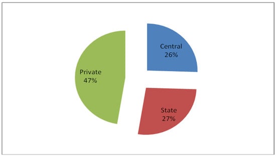
Figure 1.
Share of the electricity generation capacity of India.
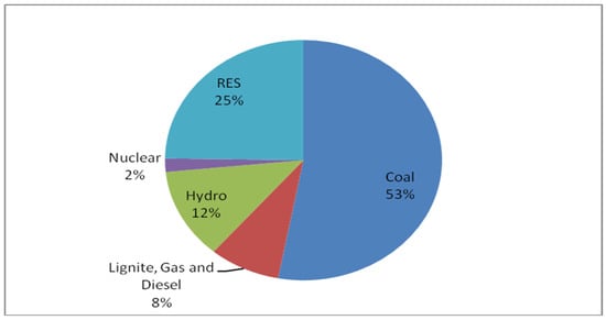
Figure 2.
Share of generation by source in India.
Electricity consumption is a dominant factor in economic growth. Previous research established that electricity availability to rural farmers was the most critical factor in India’s agricultural growth and green revolution, surpassing other factors such as the improved quality of fertilizers and farm automation equipment [13,14]. Similarly, most industrial activities, such as metal processing, cement, automobile and ancillary production, metalworking, crude extraction, and refining, are highly dependent on electricity consumption as a source of power. As depicted in Figure 3, the industrial sector consumed 42.7% of the electricity generated, followed by the domestic and agriculture sectors in 2020. India’s annual GDP growth was 8.26% in 2016 but decreased to 4.18% in 2019 due to pandemic disruptions. Regarding the future GDP, the growth of GDP will be driven by the industrial sector, thereby increasing electricity consumption (Cosmas et al., 2019) [15].
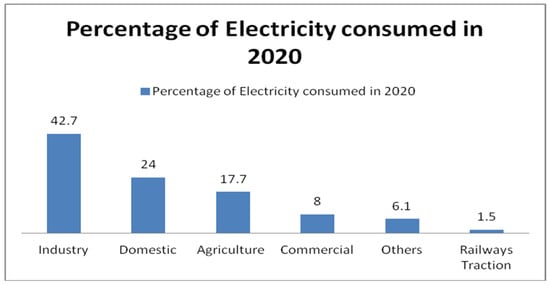
Figure 3.
Distribution of electricity consumption by sector in 2020.
Several researchers [16,17,18,19,20,21,22] established a positive correlation between uninterrupted and high-quality electric supply and an increase in the contribution of the industrial sector to national GDP growth. Based on this argument, we can summarize that electricity availability is the most crucial factor for India’s economic development and growth. With the stiff target of double-digit growth in the near future, the demand for electricity will continue to increase, resulting in a similar growth in coal consumption. Therefore, there is a need to model the growth of electricity and coal along with the industrial output for the future and implement policies for green growth in the coal sector that are specific to India’s context.
Although it is an older concept, green marketing gained prominence at the Rio + 20 conference in Brazil in 2012, where path-breaking guidelines were formulated on green economic policies [23]. The conference’s outcome document clearly emphasized the need for a green economy and green economic growth. Green growth is a set of measures that promote economic growth and development while ensuring that nature continues to provide the resources and environmental services on which our health and overall happiness depend. Green growth aims to accelerate investment and innovation that support sustainable development and create new economic opportunities. Furthermore, green strategies must lead to pro-environmental behavior from all stakeholders in the entire chain of economic activity, not limited to the reallocation of capital, labor, location, land, and technology. These strategies can lead to a greener outcome toward the development of green innovations. Green marketing strategies can demonstrate the competence of organizations and become the critical driver for influencing the entire marketing process, thereby bringing vital revenue and contributing toward making the Earth a sustainable system.
This study explored the causal relationships between coal, electricity, and industrial activity and developed policy recommendations to green the Indian coal sector. The novelty of this study lay in the use of a mix of modeling approaches, such as linear cointegration, non-linear cointegration, and ARIMA models. We assessed the forecasting performance of these models using in-sample training and testing to identify the best-performing models for predicting the values that coal, electricity, and industrial activity may take in the forecasted period. The set of modeling techniques applied in this study carries specific advantages, such as ruling out spurious relationships, capturing non-linear dynamics due to structural breaks, considering the impact of asymmetric variations, and ensuring robustness and consistency of interpretation. To the best of our knowledge, this is the first attempt of its kind. Additionally, this study considered the economic disruption caused by the COVID-19 pandemic and realigned the forecast of the economic indicators accordingly.
2. Literature Review
A large body of literature is available on the empirical analysis of energy, electricity, coal consumption, growth of economic activities, and greenhouse gas emissions. Since the industrial production index (IIP) correlates better with electricity consumption in India than GDP, we used it in our study. As we mainly examined the Granger causality association between coal production, electricity generation, and the industrial production index in the present study, we focused on studies mainly related to the Indian context. Some recent research work on the VECM are given in Table 1.

Table 1.
Recent research on the VECM.
Previous regional studies confirmed GDP growth as the main source of carbon dioxide or sulfur dioxide emissions [31,32,33]. Grossman and Krueger (1995) employed a panel dataset of different countries and established that amplified domestic production has resulted in environmental degradation. Using a nonparametric approach to panel data, [34] confirmed the affirmative and non-linear relationship between GDP and carbon emissions. However, they discarded the option of the polynomial relationship between both variables. In other words, this study did not find an environmental Kuznets curve (EKC) for the selected country. Conversely, Narayan and Narayan (2010) [35] studied the panel data of 43 growing countries and established an EKC in the long term.
In [36], researchers analyzed a panel dataset comprising eight countries and investigated the relationship between GDP, energy use, trade expansion, population, and environmental quality. They discovered that the environmental Kuznets curve (EKC) existed in two countries; however, in the long term, the association was of the inverted N-type for the other six countries. In a similar vein, de Souza et al. (2018) [37] utilized panel data from five countries to explore the impact of renewable energy on pollution levels. They posited that the use of renewable energy sources mitigates pollution, whereas the use of zero renewable energy contributes to environmental degradation. Furthermore, Mert et al. (2019) [38] used the autoregressive distributed lag (ARDL) technique to analyze data from 26 countries. They established the existence of the EKC in five countries and found that implementing pollution mitigation legislation significantly improved the environmental quality in these countries.
Mert et al. (2019) [38] used the Dumitrescu–Hurlin methodology with panel data from European countries and found that trade expansion and the use of green energy led to a decrease in the intensity of pollution in those countries. Therefore, they advocated for the industrial sector to use green energy. Balogh (2017) [39] employed the generalized method of moments (GMM) approach with GDP, FDI, tourism, agriculture, and trade expansion as variables to calculate the CO2 emissions in 168 countries. They found that the use of green and nuclear energy helped to mitigate pollution in the selected countries. These conclusions were also confirmed by Shahbaz et al. (2019) [40] in their panel data study. Sharma et al. (2020) [41] established an N-type association between GDP and CO2 emissions. Based on this argument, we decided to use the index of industrial production, electricity generation, and coal production as research variables in the present study.
3. Data Description
This study used monthly secondary coal production (CoP) data, the general industrial production index (IIPG), and electricity generation (ELG). The sample period for the research variables in this study spanned from April 1999 to December 2020. The datasets were downloaded from the indiastat.com website, which mostly collates data from India’s concerned sectoral ministry of the Government of India. Monthly coal production data (in millions of tonnes) and electricity generation data (gigawatt hours) were generated from the websites of the Ministry of Coals and the Ministry of Power, respectively. CoP and ELG were obtained after applying a natural logarithmic transformation to these two data series. The monthly index of industrial production (general) was captured from the Ministry of Statistics and Program Implementation website. The IIP (general) data were first converted to a uniform base year of 1993–1994 and subsequently applied to a natural logarithmic transformation to obtain the IIPG. The CoP, IIPG, and ELG plots and their statistical characteristics are presented in Figure 4 and Table 2.
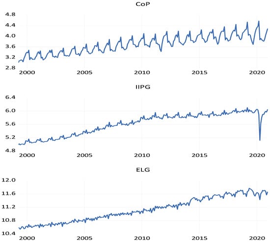
Figure 4.
Graphical presentation of research variables. There was a sharp decline in ELG from 2020 onward due to the COVID-19 pandemic.
Table 2.
Descriptive statistics of the research variables.
4. Methodology
4.1. Johansen Cointegration Test
Cointegration between two or more non-stationary series indicates a systematic co-movement between them over the long run. Engle and Granger (1987) [42] demonstrated that cointegration between two or more I(1) series might indicate (a) the absence of a spurious correlation, (b) a causal relationship in at least one direction, and (c) long-run Granger’s causality of cointegrating vectors from a vector error correction model. We applied the Johansen cointegration test [43], which is considered one of the best linear cointegration techniques, to analyze the cointegration relationships between CoP, IIPG, and ELG. The Johansen cointegration test, which was suggested by Johansen (1988) [43], is equation-based, unlike the residual-based cointegration technique similar to the one proposed by Engle and Granger (1987) [42]. We used VAR lag order selection criteria based on sequential modified LR test statistics, final prediction error, and Akaike information criterion to reduce the bias and increase the accuracy of the cointegration tests. The resulting optimal lag length is the maximum lag interval for differenced endogenous variables in the Johansen test.
The vector error correction model (VECM), rather than the VAR/Granger causality model, should be used for causality analysis of the variables. The VECM is capable of examining both short- and long-run causality analysis. The VECM captures the effect of error correction term changes and differences in independent variable lagged terms on dependent variables. The VECM can be expressed as shown in Equations (A1)–(A3) given in Appendix A.
Here, the β’s are the coefficients to be estimated, p is the optimal lag, εt−1 is the error correction term (ECT), and the ut’s are serially uncorrelated error terms. The lagged ECT coefficients’ t-statistics are used to examine long-run causality from independent to dependent variables. Similarly, lagged independent variable F-statistics may be used to examine short-run causality in the ECM. If = 0 is rejected in Equation (A1), it shall signify short-run granger causality from IIPG to CoP. The coefficient of ECT shows the speed of adjustment from the perturbed state to the equilibrium state. If = 0 is rejected in Equation (A1), this establishes the existence of a long-run causality relationship between one or more independent variables in CoP.
4.2. Regime Shift Cointegration Model
This and similar cointegration methodologies proposed by Johansen (1988) [43] and others have been criticized for being unrealistic in assuming a constant cointegrating relationship between variables over the entire data span [44]. The problem of an overgeneralized assumption becomes too acute when the period of data of the study is long. In the case of one or more structural breaks, the above cointegration tests may produce misleading results.
We applied cointegration tests with two endogenously determined regime shifts as Hatemi-j (2008) [45] suggested and is called the Hatemi-J model. The model introduces two endogenous regime shifts for slope and level slope dummies. The Hatemi-J model is given in Equation (A3).
Here, α0 is the common intercept, while α1 and α2 are the intercept dummies reflecting the first and second regime shifts’ differential repercussions over α0, respectively. β01 is the base slope, while β11 and β21 are the first and second regime shifts’ differential slope coefficients of IIPG. Similarly, β02, β12, and β22 can be defined with respect to ELG. The error term in the above Hatemi-J model is represented by εt. The endogenous regime shifts were incorporated using two dummy variables D1t and D2t, as shown below.
T1 and T2 indicate the relative timings of the two regime shifts and can have fractional values in the range (0, 1).
The Hatemi-J model uses modified ADF*, Zα*, and Zt* tests while examining the cointegration relationships in endogenous regime shifts to avoid misspecification errors in the residual-based cointegration approach.
4.3. Non-Linear Auto-Regressive Distributed Lag (NARDL) Model of Cointegration
The NARDL model was suggested by [46]. This enables simultaneous estimation of long-run and short-run asymmetric nonlinearities. The NARDL framework for CoP, IIPG, and ELG is given below.
Here, Δ signifies the first difference operator. The long-run coefficients are represented by ω1Y, ω2Y, and ω3Y, while short-run coefficients are represented by α1Y, α2Y, and α3Y. IIPGt+ and IIPGt− (say) reflect the positive and negative changes in the partial sum of IIPGt. Similarly, other partial sums can be interpreted. The null hypothesis (no asymmetric cointegration) is examined using F-statistics. For instance, for Equation (A10), H0 is ω1CoP = ω+2CoP = ω−2CoP = ω+3CoP = ω−3CoP = 0. The long- and short-run symmetries can be examined by applying the standard Wald test [46]. The long-run symmetry null hypothesis is δ+ = δ−, where δ+= −ωjY/ω1Y and δ− = −ω-jY/ω1Y, where j = 1, 2, … Similarly, the short-run symmetry null hypothesis is where j = 1, 2… for Equation (A10).
4.4. General ARIMA Model
In this study, the ARIMA technique was used for the univariate modeling of CoP, IIPG, and ELG for their possible use in out-of-sample forecasting. The general seasonal ARIMA model, can adequately explain the seasonal changes and trend effects observed practically in the time series [47]:
Here, L is the backward shift operator, d is the order of difference needed to make Xt stationary, is the moving average parameter, and represents the fixed seasonal autoregressive parameter. The Xt may be expressed as ARIMA (p, d, q) if the stationary series obtained after the d difference of Xt can be expressed as ARIMA (p, q).
5. Results
5.1. Unit Root Test
The three data series were subjected to multiple stationarity tests for robust interpretation of their order of integration. The summary results of traditional unit root tests (Augmented Dickey–Fuller—ADF, Phillips–Perron—PP, and Kwiatkowski–Phillips–Schmidt–Shin (KPSS)) and structural break unit root test [48] are presented in Table 3. The unit root tests at the level (intercept and trend) and after the first difference (intercept, no trend) majorly indicated that CoP, IIPG, and ELG were I(1) time series or non-stationary. Since linear regression using non-stationary variables may not rule out spurious relationships between variables, we decided to use a mix of linear and non-cointegration modeling techniques. The structural break unit root results suggested the possible existence of structural breaks in the three research variables, thereby justifying the use of a non-linear cointegration approach to regime shift modeling and the non-linear ARDL cointegration technique. The structural break dates for CoP, IIPG, and ELG were November 2007 (2007M11), December 2006, (2006M12), and March 2011 (2011M03), respectively.
Table 3.
Unit root tests.
5.2. Johansen Cointegration Model
Based on the selection criteria of the VAR lag order (sequential modified LR test statistics, final prediction error, and Akaike information criterion), the optimal lag length of 12 was used as the maximum lag interval for differenced endogenous variables in the Johansen test. The deterministic trend assumption of the JJ test was an intercept (no trend) in CE and no intercept in VAR (option 2) to allow for the linear deterministic trend in the data. According to trace statistics summarized in Table 4, the null hypotheses of r = 0 and r ≤ 1 were rejected against r > 0 and r > 1, respectively. The trace and maximum eigenvalue statistics were not rejected (t-statistics less than the 5% critical value) for r ≤ 2, indicating the presence of two cointegrating relationships between the research variables.
Table 4.
Results of cointegration rank test.
Since the three variables had a co-integrating relationship, the VECM was used to estimate the short-term relationship. Table 5 summarizes the long-run and short-run Granger causality using the VECM. The long-term causality ran from CoP to ELG and from IIPG to ELG. The speed of adjustment was −0.08 for ELG (for ECT-1) and −0.14 for IIPG (for ECT-2). There was bidirectional short-term causality between CoP and ELG. A significant unidirectional causality was also detected from CoP and ELG to IIPG in the short run.
Table 5.
Summary of short- and long-run Granger causality results.
5.3. Regime Shift Cointegration Model
Cointegration tests with two endogenously determined regime shifts, as suggested by [45], were applied through three models with each of CoP, IIPG, and ELG as dependent variables. The regime shift cointegration approach introduced level and slope dummy variables to determine the timing of two unknown regime shifts if they existed. Here, the null hypothesis was taken as no regime shift cointegration. The majority of test statistics (ADF, Zt*, and Zα*) for each model were rejected at the 5% significance level (refer to Table 6), which established the existence of regime shift cointegration between CoP, IIPG, and ELG.
Table 6.
Cointegration with an endogenous structural break adapted from [45].
The two models with CoP and IIPG as dependent variables (refer to panels A and B, respectively, of Table 6) revealed the same set of regime shifts in October 2011 and September 2015, while the model with ELG as a dependent variable (refer to panel C of Table 6) suggested regime shifts in April 2014 and September 2015. The elasticity estimation of F(IIPGELG, CoP) indicated that IIPG was elastic against ELG and inelastic against CoP until October 2011. The causal relationship from ELG to IIPG became inelastic from November 2011 to September 2015 and then regained elasticity afterward. For instance, a 1% increase in ELG led to 1.00%, 0.11%, and 0.84% increases in IIPG until October 2011, from November 2011 to September 2015, and from October 2015 onward, respectively. No significant variation was observed in the causal relationship elasticity from CoP to IIPG during the two regime shifts. For instance, a 1% increase in CoP resulted in a 0.23% increase in IIPG.
5.4. NARDL Cointegration
We started with the estimation of three ARDL models whose bound test results are summarized in Table 7. The models F(CoP/IIPG, ELG) and F(IIPG/ELG, CoP) qualified as bound tests of cointegration for the ARDL models. However, they could not be taken forward as they did not qualify for the diagnostic specifications (normality tests, no heteroscedasticity, no serial correlation, and Ramsey stability statistics).
Table 7.
Results of bounds tests of cointegration for the ARDL models.
Furthermore, we examined the NARDL modeling techniques suggested by [46] to overcome the constraints posed due to the assumption of ARDL, whereby negative and positive variations in independent variables have a similar effect. Table 8 contains a summary of bound test results for all NARDL models corresponding to three fixed regressor’s trend specifications: (i) restricted constant, (ii) constant, and (iii) constant and trend. The figures inside parentheses presented with the nine F-statistics are the lag order discovered by the models endogenously, with 8 and 12 as the maximum lags for the dependent and regressor variables, respectively. All these statistics were significant at the 5% level. The NARDL model F(IIPG/ELG+, ELG-, CoP+, CoP-) with IIPG as a dependent variable was dropped as it did not qualify for the diagnostic specifications. Thus, IIPG and ELG possessed NARDL relationships with CoP, while CoP and IIPG possessed a NARDL relationship with ELG.
Table 8.
Results of bound tests of cointegration for the NARDL models.
Table 8 contains the summary of the Wald tests for F(CoP/IIPG+, IIPG−, ELG+, ELG−) and F(ELG/CoP+, CoP−, IIPG+, IIPG−) in panels A and B, respectively. The panel A results show the short-run asymmetric causality from IIPG and ELG to CoP, while the panel B results show the short-run asymmetric causality from CoP and IIPG to ELG.
Table 9 contains a summary of the coefficient estimation results (panel A), long-run asymmetric effects (panel B), and statistics and diagnostics details (panel C) for the F(CoP/IIPG+, IIPG−, ELG+, ELG−) and F(ELG/CoP+, CoP−, IIPG+, IIPG−) models. The statistical and diagnostic details for the two NARDL models established the absence of misspecification errors at the 5% level of significance, thereby evidencing the accuracy of the maximum lag specification in the model building. The long-run and short-run asymmetric relationships between the variables in both these models were largely in line with the outcomes of the Wald tests. One of the insights revealed by the long-run asymmetric effects (panel B, Table 10) of the F(CoP/IIPG+, IIPG−, ELG+, ELG−) model regarded asymmetric causality existence from IIPG to CoP at the 1% significance level. For instance, a 1% increase (decrease) in IIPG resulted in a 0.40% (0.35%) increase (decrease) in CoP. The F(ELG/CoP+, CoP−, IIPG+, IIPG−) model showed asymmetric causality from IIPG+ to ELG. Similarly, the short-run asymmetric effects analysis revealed that a 1% increase (decrease) in IIPG decreased (increased) CoP by 0.83% (0.83%), while a 1% increase (decrease) in ELG decreased (decreased) CoP by 0.37% (2.11%). In the case of the F(ELG/CoP+, CoP−, IIPG+, IIPG−) model, the 1% short-run increase (decrease) in CoP increased (decreased) ELG by 2.16% (2.70%), while a 1% increase (decrease) in IIPG decreased (decreased) ELG by 0.05% (0.79%).
Table 9.
Wald tests showed long-run and short-run asymmetric cointegration dynamics.
Table 10.
NARDL cointegration results.
5.5. Forecasting
5.5.1. Partitioning the Data Set
The dataset spanning from April 1999 to December 2020 (261 months) was divided into three subsets. The first subset, from April 1999 to December 2017, was used as the training dataset. The second subset, from January 2018 to December 2019, was used as the testing dataset. The third subset, from January 2020 to December 2020, represented the COVID-19 period, which witnessed significant socio-economic disruption. This period’s data may have resulted in significant deviations from seasonal, short-run, and long-run trends. Therefore, the COVID-19 data was excluded from both the training and testing datasets to minimize its influence on the forecasting model development. This exclusion was made to generate the forecasting data from January 2021 to December 2025 (60 months). In this study, we utilized the mean absolute error, mean absolute percentage error, and root mean squared error to evaluate the forecasting performance of each model.
5.5.2. ARIMA Forecasting
To compensate for the limitation of out-of-sample forecasting in the Johansen cointegration models, we employed ARIMA univariate forecasting techniques for the research variables. Since the research variables were I(1) in nature, we converted them into respective differenced series. The ARIMA model development for D(CoP) involved three steps: (i) identifying a better/appropriate ARIMA model based on the sample autocorrelation function and partial autocorrelation function to select p (the autoregressive order) and q (the moving average order) of the model, (ii) estimating the coefficients using the maximum likelihood technique and dropping coefficients lacking significance, and (iii) adding moving average and autoregressive variables and evaluating the coefficient estimation. Steps (ii) and (iii) were iterated until the model residuals acquired random or white noise characteristics. Similarly, ARIMA models for IIPG and ELG were developed by following the same three steps.
Panel A of Table 11 presents the final univariate ARIMA models identified for all three variables. The MAE, MAPE, and RMSE values of the actual vs. forecasted training data (April 1999 to December 2017) are also presented in panel B, indicating that ELG displayed better forecasting performance than CoP and IIPG.
Table 11.
ARIMA coefficient estimation of research variables.
The forecasting performance results (MAE, MAPE, and RMSE calculations) of the three ARIMA models using testing, training, and COVID-19 data are presented in panel B of Table 11. Comparing the forecasting performance of Johansen cointegration and ARIMA forecasting, we found that both techniques had similar forecasting capabilities.
5.5.3. Cointegration Forecasting Performance
Panel A of Table 12 presents the forecasting performance results (MAE, MAPE, and RMSE calculations) of the Johansen linear cointegration model, while panels A and B of Table 13 summarize the corresponding results for the regime shift cointegration and NARDL cointegration models, respectively. The cointegration model specifications are covered in Section 5.2, Section 5.3 and Section 5.4 and are not repeated here for the sake of brevity. Of the three cointegration models, only the Johansen cointegration model is capable of performing out-of-sample forecasting. The regime shift cointegration and NARDL cointegration models can be used as forecasting models if the independent variables are forecasted using other techniques.
Table 12.
Post-facto forecasting performance of the Johansen cointegration and ARIMA models.
Table 13.
Post-facto forecasting performance of the regime shift and NARDL models.
5.5.4. Identifying the Superior Model
During the testing data period, the NARDL cointegration model exhibited the best forecasting performance for CoP, followed by the Johansen cointegration model (refer to Table 13). The comparison of the IIPG forecasting performance displayed by the four models during the testing data period indicated that the regime shift cointegration model was the best performer, followed by the Johansen cointegration model. Similarly, ARIMA displayed the best forecasting capabilities for ELG during the testing data period, followed by the NARDL cointegration model.
Given the lack of out-of-sample forecasting capabilities of the regime shift and NARDL cointegration models, we recommend using the Johansen cointegration model for forecasting CoP and IIPG. For ELG, ARIMA was the best-suited model for forecasting. Overall, the Johansen cointegration model appeared to be the most reliable and accurate forecasting model for the three variables, given its ability to perform out-of-sample forecasting.
The forecasting performance results of the four models for each variable during the COVID-19 period (January 2020 to December 2020) exhibited a distinct increase compared with their respective test data period performance, thereby establishing the socio-economic disruption effect on the three research variables. For IIPG, no substantial difference in the forecasting performance of the four models was observed between the testing and COVID-19 periods. However, the forecasting performance of the regime shift cointegration and NARDL models for CoP and ELG was distinctly poorer during the COVID-19 period compared with the testing period.
5.5.5. Best Model Forecasting
The combined in-sample and forecasted out-of-sample plots for CoP, IIPG, and ELG are shown in Figure 5. The monthly in-sample average values of the three research variables (2015 to 2020) and their forecasted monthly average values (2021 to 2025) are presented in Table 14.
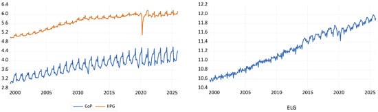
Figure 5.
Plots of research variables during the sample and forecasted period.
Table 14.
Actual monthly average values vs. forecasted average values.
6. Discussion
This study aimed to examine (i) the causal relationships between the monthly data of coal production (CoP), a general index of industrial production (IIPG), and electricity generation (ELG) from April 1999 to December 2020; (ii) verify whether the COVID-19 pandemic impacted the observed historical trends in the research variables and their interrelatedness; and (iii) estimate the three research variables from January 2021 to December 2025. To decode the dynamics of CoP, IIPG, and ELG, a mix of linear cointegration and non-linear cointegration models were used. Next, the forecasting performances of the three cointegration and autoregressive integrated moving average (ARIMA) models were compared based on in-sample training data points to identify the best forecasting model candidate for each research variable. Finally, the respective best forecasting model was applied to forecast the 60 data points for each variable.
Initially, we applied the linear cointegration model to the research variables, as they possessed I(1) characteristics. The linear cointegration technique revealed bidirectional short-run causality between CoP and ELG, indicating the continued impact of coal production on electricity generation in India. A sudden reduction in coal production due to environmental concerns may have adverse effects on electricity generation or increase dependence on coal imports. Moreover, the reverse causality from ELG to CoP suggested that an increase in electricity demand may call for more coal mining activities. Alternatively, policymakers may need to shift toward renewable energy sources. The linear cointegration technique established the existence of two long-run co-movement causalities from CoP and ELG to IIPG with moderate speeds of adjustment (−0.14 and −0.21, respectively). Additionally, significant unidirectional causalities were detected from CoP to IIPG and ELG to IIPG. Therefore, there existed causality from CoP to IIPG and ELG to IIPG both in the long run and short run. These findings align with previous studies [50,51] and carry substantial policy implications, as policymakers need to synergize the connectedness between CoP and ELG to accelerate IIPG.
The cointegration tests suggested by Hatemi-j (2008) [45] established the presence of two endogenously determined regime shift cointegration relationships in each of the three models with CoP, IIPG, and ELG as dependent variables. October 2011 was identified as the regime shift location by the two models with CoP and IIPG as dependent variables. The monthly plots of IIPG displayed a local decline in growth trend in 2011, which may be attributed to the overall fall in GDP to 5.3% compared with 8.5% in 2010. This decline in GDP growth was caused by prolonged policy paralysis (coalition government politics), lack of ease of business environment (including delayed tax reforms), reduced domestic demand due to increasing inflation, weakened currency, and reduced external demand due to the US and Euro crises, which was consistent with the findings of Sen and Sen (2019) [52]. It severely impacted the industrial sector’s performance. The CoP plot also showed a local dip in the growth trend in 2011, which was accurately captured as a regime shift location by the CoP regime shift cointegration model.
The government’s corrective actions resulted in the gradual recovery of the Indian economy. After 2011, the GDP growth gradually increased and peaked at 8.26% in 2016. The new government formed in 2014 successfully created a positive atmosphere through a series of infrastructure development initiatives and policy reforms. This was reflected in IIPG, which also showed gradual improvement until 2015 before rapidly improving in 2016. The regime shift location of April 2014 captured by the ELG model was consistent with the ELG plot, as marked by a shift to a higher growth pedestal and a change in seasonal characteristics. This increased shift in ELG was observed around 2019 before declining due to the overall slowdown of the Indian economy in 2019 and the COVID-19 pandemic’s effect in 2020. The CoP plot also showed a local increase in its growth trend in 2015, which continued until 2017 before experiencing a fall.
In line with the findings of linear cointegration, the regime shift model of IIPG (as a dependent variable) established a causal relationship between ELG and CoP to IIPG [29,53]. However, this regime shift model revealed additional insights into how the relationship between ELG to IIPG was elastic until October 2011, changed to an inelastic nature from November 2011 to September 2015, and then partially regained elasticity afterward. IIPG’s increasing trend was moderate from 2011 to 2015; however, ELG continued with its regular growth trend. Thus, the elasticity of CoP reduced in this period. The causal relationship elasticity from CoP to IIPG during the two regime shifts did not show significant variations. For instance, a 1% increase in CoP resulted in a 0.23% increase in IIPG.
The NARDL techniques revealed that CoP and ELG, as dependent variables, possessed asymmetric cointegration relationships with their respective independent variables. The short-run asymmetric causality findings from Wald tests aligned with the findings from coefficient estimation analysis of CoP and ELG asymmetric cointegration models. The long-run asymmetric relationship analysis in the CoP (as a dependent variable) model indicated that a 1% increase (decrease) in IIPG resulted in a 0.40% (0.35%) increase (decrease) in CoP. This has important policy implications as it suggests that positive and negative changes in IIPG will have a different magnitude of impact on CoP. The short-run asymmetric effects analysis revealed that a 1% increase (decrease) in IIPG decreased (increased) CoP by 0.83% (0.83%), while a 1% increase (decrease) in ELG decreased (decreased) CoP by 0.37% (2.11%). This analysis suggested the combined usage of short-run and long-run asymmetric variations in IIPG and ELG to evaluate their impact on coal production (CoP variable) planning.
The ELG NARDL model showed asymmetric long-run causality from IIPG+ to ELG, wherein a 1% increase in IIPG required a 0.42% increase in electricity generation, which was consistent with previous studies [8,15,27]. This provides an important indicator to strategize electricity generation to meet the increase in the index of industrial production. A 1% short-run increase (decrease) in CoP increased (decreased) ELG by 2.16% (2.70%), while a 1% increase (decrease) in IIPG decreased (decreased) ELG by 0.05% (0.79%). This analysis suggested the combined usage of short-run and long-run asymmetric variations in IIPG and CoP to evaluate their impact on electricity generation (ELG variable) planning.
ARIMA, which is a popular univariate model, and the three multivariate cointegration models were applied to the training data series (April 1999 to December 2017) to generate respective forecasting models. Based on the post-facto forecasting performance of these models on the testing data (January 2018 to December 2019), the Johansen cointegration model emerged as the best forecasting model for CoP and IIPG, while ARIMA was the best-suited model for forecasting ELG, which was consistent with the results found by Dua et al. (2023) and Telarico (2023) [54,55]. The forecasting performance of the four models for each variable during the COVID-19 period (January 2020 to December 2020) showed a distinct decline compared with their respective test data period performance, thereby establishing the socio-economic disruption effect in the three research variables. The monthly in-sample average values of the three research variables (2015 to 2020) and their forecasted monthly average values (2021 to 2025) are presented in Table 14. Based on the above estimates, India needs to plan to produce 67.84 million tonnes of coal and generate 150679 GWh of electricity units to achieve a 156.32 general index of industrial production compared with its present value of 122.22.
7. Conclusions and Policy Implications
Thermal power generation based on coal will remain the backbone of electricity generation in India for the next decade. However, this can result in increased carbon emissions and environmental degradation due to the expected increase in coal production. Therefore, we propose several policy recommendations to promote green and sustainable coal usage in the entire coal cycle chain, from coal mining to coal combustion:
- The greening of the Indian coal life cycle is highly dependent on cutting-edge technological innovations. The adoption of new technology and innovation is driven by three factors: ease of implementation, economic viability, and environmental sustainability. There is a wide range of clean coal technologies being adopted in India, such as fluidized bed combustion (successfully implemented in 36 power plants), supercritical and ultra-supercritical boiler technology (successfully implemented in 11 power plants), and oxyfuel technology (still in the early research phase).
- Promoting technological research, innovation, and cutting-edge research in coal conversion technologies can potentially have a significant impact on greening the coal combustion cycle, thereby mitigating the after-effects of coal combustion. Therefore, policies should be implemented to provide an ecosystem to nurture research programs. Single-window clearance for regulatory measures should be put in place to facilitate fast adoption and commercialization.
- In the context of green coal usage, emphasis should be placed on improving coal mining, coal washing, waste disposal, and coal transportation. Table 15 shows areas of improvement in the coal usage cycle.
Table 15. Areas of improvement in the coal use cycle.
Author Contributions
Conceptualization, N.D.; Methodology, A.M. and P.C.; Software, A.M.; Validation, P.C.; Formal analysis, P.C.; Investigation, P.C.; Resources, A.M.; Writing – original draft, A.M.; Visualization, P.C.; Supervision, N.D. All authors have read and agreed to the published version of the manuscript.
Funding
This research received no external funding.
Institutional Review Board Statement
Not applicable.
Informed Consent Statement
Not applicable.
Data Availability Statement
The relevant experiments of this study are still in progress. If you need our data for relevant research, you can contact the corresponding author of this article.
Conflicts of Interest
The authors declare that they have no known competing financial interests or personal relationships that may appear to influence the work reported in this paper.
Appendix A
D1t = 0 if t
≤ [nT1] and 1 if t > [nT1]
D2t = 0 if t
≤ [nT2] and 1 if t > [nT2]
ADF* = inf ADF(τ), where
τ ∈ T
Zt* = inf Zt
(τ), where τ ∈ T
Zα* = inf Zα
(τ), where τ ∈ T
References
- Udemba, E.N.; Güngör, H.; Bekun, F.V.; Kirikkaleli, D. Economic performance of India amidst high CO2 emissions. Sustain. Prod. Consum. 2021, 27, 52–60. [Google Scholar] [CrossRef]
- Babatunde, O.M.; Munda, J.L.; Hamam, Y. A comprehensive state-of-the-art survey on power generation expansion planning with intermittent renewable energy source and energy storage. Int. J. Energy Res. 2019, 43, 6078–6107. [Google Scholar] [CrossRef]
- Peng, T.; Ou, X.; Yan, X. Development and application of an electric vehicles life-cycle energy consumption and greenhouse gas emissions analysis model. Chem. Eng. Res. Des. 2018, 131, 699–708. [Google Scholar] [CrossRef]
- Kaya, Y.; Yokobori, K. Environment, Energy, and Economy: Strategies for Sustainability; United Nations University Press: Tokyo, Japan, 1997. [Google Scholar]
- Eggleston, H.; Buendia, L.; Miwa, K.; Ngara, T.; Tanabe, K. 2006 IPCC Guidelines for National Greenhouse Gas Inventories; Institute for Global Environmental Strategies: Kanagawa, Japan, 2006. [Google Scholar]
- Hwang, Y.; Um, J.-S.; Hwang, J.; Schlüter, S. Evaluating the causal relations between the Kaya Identity Index and ODIAC-based fossil fuel CO2 flux. Energies 2020, 13, 6009. [Google Scholar] [CrossRef]
- Yan, Q.; Wang, Y.; Baležentis, T.; Sun, Y.; Streimikiene, D. Energy-related CO2 emission in China’s provincial thermal electricity generation: Driving factors and possibilities for abatement. Energies 2018, 11, 1096. [Google Scholar] [CrossRef]
- Wang, Z.; Zhu, Y. Do energy technology innovations contribute to CO2 emissions abatement? A spatial perspective. Sci. Total Environ. 2020, 726, 138574. [Google Scholar] [CrossRef] [PubMed]
- Kamboj, P.; Tongia, R. Indian Railways and Coal: An Unsustainable Interdependency. 2018. Available online: https://www.brookings.edu/articles/indian-railways-and-coal/ (accessed on 24 March 2022).
- Worrall, L.; Whitley, S.; Garg, V.; Krishnaswamy, S.; Beaton, C. India’s Stranded Assets: How Government Interventions Are Propping up Coal Power; Overseas Development Institute: London, UK, 2018. [Google Scholar]
- Bhatt, R.P. Climate change assessment, impacts of global warming, projections and mitigation of ghg emissions endorsing green energy. Int. Educ. Sci. Res. J. 2018, 4, 33–48. [Google Scholar]
- Mishra, A.; Das, N.; Mishra, B. Sustainable Strategies for Indian Coal Sector: An Econometric Analysis Approach. 2022. Available online: https://www.researchsquare.com/article/rs-2290236/v1 (accessed on 1 March 2023).
- Jha, G.K.; Pal, S.; Singh, A. Changing energy use pattern and the demand projection for Indian agriculture. Agric. Econ. Res. Rev. 2012, 25, 75–82. [Google Scholar]
- Dogan, E.; Sebri, M.; Turkekul, B. Exploring the relationship between agricultural electricity consumption and output: New evidence from Turkish regional data. Energy Policy 2016, 95, 370–377. [Google Scholar] [CrossRef]
- Cosmas, N.C.; Chitedze, I.; Mourad, K.A. An econometric analysis of the macroeconomic determinants of carbon dioxide emissions in Nigeria. Sci. Total Environ. 2019, 675, 313–324. [Google Scholar] [CrossRef]
- Allcott, H.; Collard-Wexler, A.; O’Connell, S.D. How do electricity shortages affect industry? Evidence from India. Am. Econ. Rev. 2016, 106, 587–624. [Google Scholar] [CrossRef]
- Beenstock, M.; Goldin, E.; Haitovsky, Y. The cost of power outages in the business and public sectors in Israel: Revealed preference vs. subjective valuation. Energy J. 1997, 18, 39–62. [Google Scholar] [CrossRef]
- Cole, M.A.; Elliott, R.J.; Occhiali, G.; Strobl, E. Power outages and firm performance in Sub-Saharan Africa. J. Dev. Econ. 2018, 134, 150–159. [Google Scholar] [CrossRef]
- Rud, J.P. Electricity provision and industrial development: Evidence from India. J. Dev. Econ. 2012, 97, 352–367. [Google Scholar] [CrossRef]
- Saxena, A.; Gopal, I.; Ramanathan, K.; Jayakumar, M.; Prasad, N.; Sharma, P. Transitions in Indian Electricity Sector 2017–2030. Energy and Resource Institute. 2017; 28p. Available online: https://www.teriin.org/files/transition-report/files/downloads/Transitions-in-Indian-Electricity-Sector_Report.pdf (accessed on 1 March 2023).
- Sullivan, M.J.; Vardell, T.; Johnson, M. Power interruption costs to industrial and commercial consumers of electricity. In Proceedings of the 1996 IAS Industrial and Commercial Power Systems Technical Conference, New Orleans, LA, USA, 6–9 May 1996. [Google Scholar]
- Tishler, A. Optimal production with uncertain interruptions in the supply of electricity: Estimation of electricity outage costs. Eur. Econ. Rev. 1993, 37, 1259–1274. [Google Scholar] [CrossRef]
- Fulton, S.C.; De Silva, L.; Anton, D. Twenty years after the rio earth summit: What is the agenda for the 2012 United Nations Conference on Sustainable Development. In American Society of International Law, Proceedings of the Annual Meeting; Cambridge University Press: Cambridge, UK, 2012. [Google Scholar]
- Gyamerah, S.A.; Gil-Alana, L.A. A multivariate causality analysis of CO2 emission, electricity consumption, and economic growth: Evidence from Western and Central Africa. Heliyon 2023, 9, e12858. [Google Scholar] [CrossRef] [PubMed]
- Acaroğlu, H.; Kartal, H.M.; García Márquez, F. Testing the environmental Kuznets curve hypothesis in terms of ecological footprint and CO2 emissions through energy diversification for Turkey. Environ. Sci. Pollut. Res. 2023, 30, 1–16. [Google Scholar] [CrossRef]
- Singh, A.; Lal, S.; Kumar, N.; Yadav, R.; Kumari, S. Role of nuclear energy in carbon mitigation to achieve United Nations net zero carbon emission: Evidence from Fourier bootstrap Toda-Yamamoto. Environ. Sci. Pollut. Res. 2023, 30, 46185–46203. [Google Scholar] [CrossRef]
- Hassan, M.S.; Mahmood, H.; Javaid, A. The impact of electric power consumption on economic growth: A case study of Portugal, France, and Finland. Environ. Sci. Pollut. Res. 2022, 29, 45204–45220. [Google Scholar] [CrossRef]
- Raza, M.Y.; Khan, A.N.; Khan, N.A.; Kakar, A. The role of food crop production, agriculture value added, electricity consumption, forest covered area, and forest production on CO2 emissions: Insights from a developing economy. Environ. Monit. Assess. 2021, 193, 1–16. [Google Scholar] [CrossRef]
- Ma, X.; Fan, Y.; Shi, F.; Song, Y.; He, Y. Research on the relation of Economy-Energy-Emission (3E) system: Evidence from heterogeneous energy in China. Environ. Sci. Pollut. Res. 2022, 29, 62592–62610. [Google Scholar] [CrossRef]
- Shakeel, M. Economic output, export, fossil fuels, non-fossil fuels and energy conservation: Evidence from structural break models with VECMs in South Asia. Environ. Sci. Pollut. Res. 2021, 28, 3162–3171. [Google Scholar] [CrossRef]
- Holtz-Eakin, D.; Selden, T.M. Stoking the fires? CO2 emissions and economic growth. J. Public Econ. 1995, 57, 85–101. [Google Scholar] [CrossRef]
- Xepapadeas, A. Economic development and environmental pollution: Traps and growth. Struct. Chang. Econ. Dyn. 1997, 8, 327–350. [Google Scholar] [CrossRef]
- Grossman, G.M.; Krueger, A.B. Economic growth and the environment. Q. J. Econ. 1995, 110, 353–377. [Google Scholar] [CrossRef]
- Azomahou, T.; Laisney, F.; Van, P.N. Economic development and CO2 emissions: A nonparametric panel approach. J. Public Econ. 2006, 90, 1347–1363. [Google Scholar] [CrossRef]
- Narayan, P.K.; Narayan, S. Carbon dioxide emissions and economic growth: Panel data evidence from developing countries. Energy Policy 2010, 38, 661–666. [Google Scholar] [CrossRef]
- Onafowora, O.A.; Owoye, O. Bounds testing approach to analysis of the environment Kuznets curve hypothesis. Energy Econ. 2014, 44, 47–62. [Google Scholar] [CrossRef]
- De Souza, E.S.; Freire, F.D.S.; Pires, J. Determinants of CO2 emissions in the MERCOSUR: The role of economic growth, and renewable and non-renewable energy. Environ. Sci. Pollut. Res. 2018, 25, 20769–20781. [Google Scholar] [CrossRef] [PubMed]
- Mert, M.; Bölük, G.; Çağlar, A.E. Interrelationships among foreign direct investments, renewable energy, and CO2 emissions for different European country groups: A panel ARDL approach. Environ. Sci. Pollut. Res. 2019, 26, 21495–21510. [Google Scholar] [CrossRef]
- Balogh, J.M. Determinants of CO2 Emission, in Determinants of CO2 Emission: Balogh, Jeremiás Máté. 2017. Available online: https://www.zbw.eu/econis-archiv/bitstream/11159/1311/1/1005319871.pdf (accessed on 20 March 2022).
- Shahbaz, M.; Balsalobre-Lorente, D.; Sinha, A. Foreign direct Investment–CO2 emissions nexus in Middle East and North African countries: Importance of biomass energy consumption. J. Clean. Prod. 2019, 217, 603–614. [Google Scholar] [CrossRef]
- Sharma, R.; Kautish; Uddin, G.S. Do the international economic endeavors affect CO2 emissions in open economies of South Asia? An empirical examination under nonlinearity. Manag. Environ. Qual. Int. J. 2020, 31, 89–110. [Google Scholar] [CrossRef]
- Engle, R.F.; Granger, C.W. Co-integration and error correction: Representation, estimation, and testing. Econom. J. Econom. Soc. 1987, 55, 251–276. [Google Scholar] [CrossRef]
- Johansen, S. Statistical analysis of cointegration vectors. J. Econ. Dyn. Control 1988, 12, 231–254. [Google Scholar] [CrossRef]
- Bondia, R.; Ghosh, S.; Kanjilal, K. International crude oil prices and the stock prices of clean energy and technology companies: Evidence from non-linear cointegration tests with unknown structural breaks. Energy 2016, 101, 558–565. [Google Scholar] [CrossRef]
- Hatemi-j, A. Tests for cointegration with two unknown regime shifts with an application to financial market integration. Empir. Econ. 2008, 35, 497–505. [Google Scholar] [CrossRef]
- Shin, Y.; Yu, B.; Greenwood-Nimmo, M. Modelling asymmetric cointegration and dynamic multipliers in a nonlinear ARDL framework. In Festschrift in Honor of Peter Schmidt: Econometric Methods and Applications; Springer: New York, NY, USA, 2014; pp. 281–314. [Google Scholar]
- Rallapalli, S.R.; Ghosh, S. Forecasting monthly peak demand of electricity in India—A critique. Energy Policy 2012, 45, 516–520. [Google Scholar] [CrossRef]
- Bai, J.; Perron, P. Computation and analysis of multiple structural change models. J. Appl. Econom. 2003, 18, 1–22. [Google Scholar] [CrossRef]
- Pesaran, M.H.; Shin, Y.; Smith, R.J. Bounds testing approaches to the analysis of level relationships. J. Appl. Econom. 2001, 16, 289–326. [Google Scholar] [CrossRef]
- Alam, M.J.; Begum, I.A.; Buysse, J.; Van Huylenbroeck, G. Energy consumption, carbon emissions and economic growth nexus in Bangladesh: Cointegration and dynamic causality analysis. Energy Policy 2012, 45, 217–225. [Google Scholar] [CrossRef]
- Bekun, F.V.; Agboola, M.O. Electricity consumption and economic growth nexus: Evidence from Maki cointegration. Eng. Econ. 2019, 30, 14–23. [Google Scholar] [CrossRef]
- Sen, S.; Sen, A. India Emerging: From Policy Paralysis to Hyper Economics; Bloomsbury Publishing: London, UK, 2019. [Google Scholar]
- Raza, M.Y. Towards a sustainable development: Econometric analysis of energy use, economic factors, and CO2 emission in Pakistan during 1975–2018. Environ. Monit. Assess. 2022, 194, 73. [Google Scholar] [CrossRef] [PubMed]
- Dua, P.; Ranjan, R.; Goel, D. Forecasting the INR/USD exchange rate: A BVAR framework. In Macroeconometric Methods: Applications to the Indian Economy; Springer: Singapore, 2023; pp. 183–224. [Google Scholar]
- Telarico, F.A. Simplifying and Improving: Revisiting Bulgaria’s Revenue Forecasting Models. arXiv Prepr. 2023, arXiv:2303.09405. [Google Scholar]


Disclaimer/Publisher’s Note: The statements, opinions and data contained in all publications are solely those of the individual author(s) and contributor(s) and not of MDPI and/or the editor(s). MDPI and/or the editor(s) disclaim responsibility for any injury to people or property resulting from any ideas, methods, instructions or products referred to in the content. |
© 2023 by the authors. Licensee MDPI, Basel, Switzerland. This article is an open access article distributed under the terms and conditions of the Creative Commons Attribution (CC BY) license (https://creativecommons.org/licenses/by/4.0/).