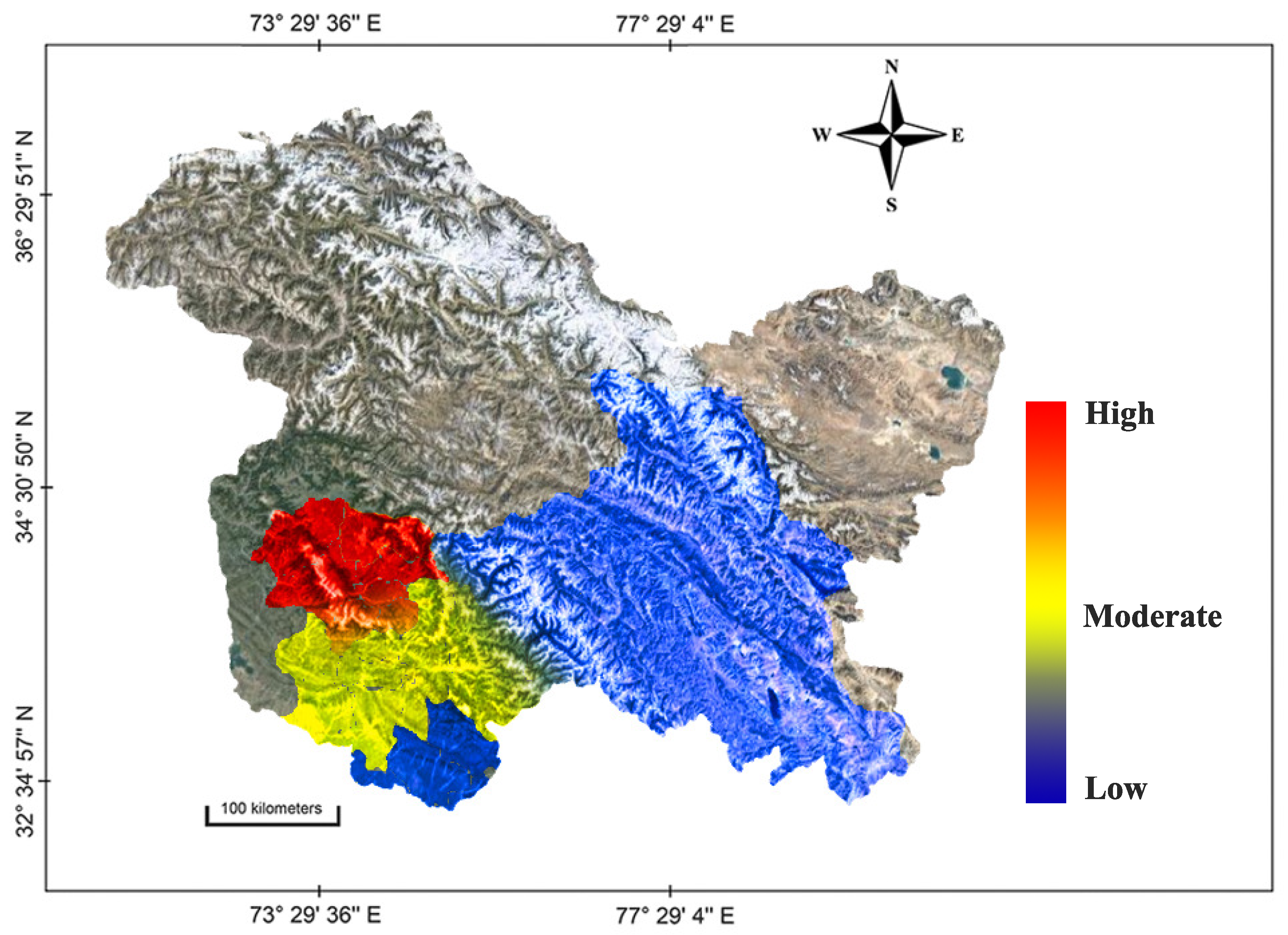
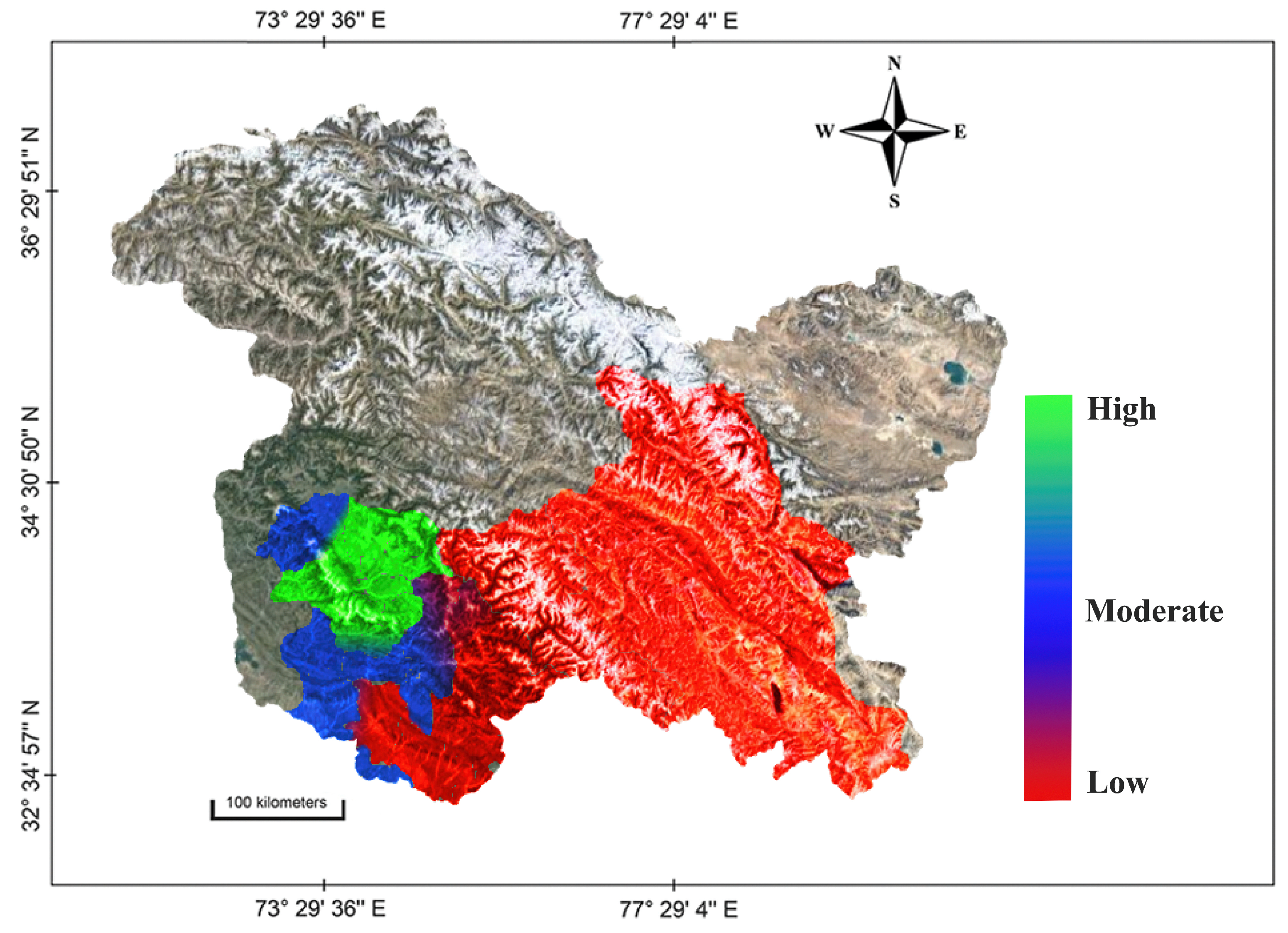
Abstract
Climate stress poses a threat to the agricultural sector, which is vital for both the economy and livelihoods in general. Quantifying its risk to food security, livelihoods, and sustainability is crucial. This study proposes a framework to estimate the impact climate stress on agriculture in terms of three objectives: assessing the regional vulnerability (exposure, sensitivity, and adaptive capacity), analysing the climate variability, and measuring agricultural performance under climatic stress. The vulnerability of twenty-two sub-regions in Jammu, Kashmir, and Ladakh is assessed using indicators to determine the collective susceptibility of the agricultural framework to climate change. An index-based approach with min–max normalization is employed, ranking the districts based on their relative performances across vulnerability indicators. This work assesses the impact of socio-economic and climatic indicators on the performance of agricultural growth using the benchmark Ricardian approach. The parameters of the agricultural growth function are estimated using a linear combination of socio-economic and exposure variables. Lastly, the forecasted trends of climatic variables are examined using a long short-term memory (LSTM)-based recurrent neural network, providing an annual estimate of climate variability. The results indicate a negative impact of annual minimum temperature and decreasing land holdings on agricultural GDP, while cropping intensity, rural literacy, and credit facilities have positive effects. Budgam, Ganderbal, and Bandipora districts exhibit higher vulnerability due to factors such as low literacy rates, high population density, and extensive rice cultivation. Conversely, Kargil, Rajouri, and Poonch districts show lower vulnerability due to the low population density and lower level of institutional development. We observe an increasing trend of minimum temperature across the region. The proposed LSTM synthesizes a predictive estimate across five essential climate variables with an average overall root mean squared error (RMSE) of 0.91, outperforming the benchmark ARIMA and exponential-smoothing models by 32–48%. These findings can guide policymakers and stakeholders in developing strategies to mitigate climate stress on agriculture and enhance resilience.
1. Introduction
An increasing footprint of climatic variability has the potential to impact billions of people in terms of how they secure their sustenance. However, the implications of climate variability can vary in magnitude and severity. A global climate change phenomenon, as specified by the Intergovernmental Panel on Climate Change (IPCC) [1], refers to
“a change in the state of the climate that can be identified by changes in the mean and/or the variability of its properties, and that persists for an extended period, typically decades or longer”.
Researchers have been studying the effects of such dynamics that alter the configuration of the atmosphere for decades [2]. The progressively receding ice caps [3], rising sea levels, and rising global temperatures [4] provide a nominal estimate of changing environmental conditions. A plethora of such manifestations is attributed to climate change, like the increase in the incidence and number of extreme events, record temperatures [5], intense rainfalls, hailstorms, floods, droughts [6], and the outbreak of pests and diseases [7]. Severe exposure to such conditions may have long- and short-term repercussions on the economy [8] and livelihood. Crop efficiency and production have been observed to be influenced antagonistically as a consequence of climatic variability [9,10], increasing food and livelihood security issues. The thrust towards industrial modernization has already taken a heavy toll on plant and animal diversity. Long-term climatic stress could influence agriculture and horticulture in various ways, incorporating changes in average temperatures, patterns of precipitation, carbon dioxide concentration in the atmosphere [5], the nutritional quality of certain foods, water availability, agricultural productivity, and the growth of essential crops with a significant deterioration of soil. On the other hand, agriculture is the principal way in which land is used worldwide. About 1.2–1.5 billion hectares of land is under harvest, with another 3.5 billion hectares [11] being grazed. People utilize approximately another 4 billion hectares [11] of forest territory to different degrees [12,13]. Ensuring food security to accommodate the anticipated needs of the increasing global population is, thus, ineluctable. Agriculture is a requisite economic activity supporting the heavy burden of the working populace in India (), although its share in the country’s GDP is declining. Moderate developments in the agrarian segment, in addition to changes in the climate, must be subject of significant consideration as they are closely linked to the food security and poverty status of a dominant part of the populace [14,15,16]. The dependence of the mass on farming practices and the risk of instability in agricultural production due to accumulating climatic stress increases the vulnerability of farmers and threat to the economy, development, and sustainability.
There are three main ways to address the threat of climate stress on the agricultural paradigm, namely (i) proactively predicting the implications of climate change on agriculture; (ii) actively studying the existing observable or perceivable effects of climate change; and (iii) passively framing adaptation policies for its mitigation measures. Our work focuses on the first two schemes of analysing climate change in terms of the three following objectives, namely characterising the vulnerability of the region to climate change; observing the forecasted trends of climate variables; and analysing the performance of agriculture in the current climatic scenario. Vulnerability assessment estimates the extent of climate change hazard, and is defined as the susceptibility and degree of risk of the region towards the impacts of long-term climatic variability, which depends on various geographic, economic, cultural, social, demographic, governance, institutional, and environmental factors [17]. The determinant variables and methodologies of estimating the vulnerability vary across studies [18,19]. A comprehensive assessment of the vulnerability of a system/region to climate change is recognized [1] as a three-fold process, namely assessments of sensitivity, exposure, and adaptive capacity variables. Exposure indicates the rate of climate variation [20] to which a region/system is exposed. Sensitivity specifies the degree to which a region/system is affected (positively or negatively, directly or indirectly) [17] and is a function of climate-related stimuli [20]. The response of the region/system that defines its recovery tendency from the effects of climate change in terms of countermeasures, potential, resources, behaviour, and technology is measured as adaptive capacity.
Deep learning has emerged as a powerful tool that has revolutionized various fields, including healthcare [21,22,23,24], education [25], and agriculture [26,27,28,29]. Its ability to process vast amounts of data and extract meaningful patterns has paved the way for transformative advancements [30]. In agriculture, deep learning has played a pivotal role in optimizing crop yields [26,31], monitoring soil conditions [32], and detecting pests and diseases early on, leading to increased productivity and sustainable practices. Statistical methods and deep learning has played a crucial role in assessing the extent of the vulnerability of agriculture to climate change, offering valuable insights into the potential impacts on crop production and guiding adaptation strategies [33,34]. By leveraging its ability to analyse complex datasets, deep learning algorithms can process diverse sources of information such as climate data, satellite imagery, and historical agricultural records. These models can identify intricate patterns and relationships that traditional statistical approaches may overlook, enabling a more accurate estimation of climate variability. One area where deep learning has made significant contributions is in crop yield prediction under climate change scenarios [35]. By training models on historical climate and agricultural data, deep learning algorithms can learn patterns and correlations that help estimate future yields [36]. These models can take into account various climate variables such as temperature, rainfall, and humidity. By incorporating these multidimensional inputs, deep learning models can provide the more precise predictions of crop yields under different climate change scenarios, helping farmers and policymakers understand the potential risks and plan accordingly. Recurrent networks in deep-learning are a valuable tool in estimating the extent of climate variability due to their ability to model temporal sequences, and identify intricate patterns and relationships that traditional methods may miss. This enables more accurate predictions of climate distributions, and helps identify the regions and crops that are most at risk. Deep learning’s capability to detect non-linear relationships and analyse historical trends contributes to a comprehensive understanding of the impact of climate change on agriculture, assisting in the development of effective adaptation strategies.
The aim of this paper is to assess the dynamics of agriculture-driven regions to climate change and their corresponding resilience. The significant contributions of this work are listed below:
- 1.
- In this work, a standard dataset comprising forty-two determinant indicators was curated from the records of Digest of Statistics (Jammu and Kashmir) [37] for the years 1983 to 2020, in addition to five exposure indicators from NASA LaRC POWER [38] for the years 1983–2022 across twenty-two sub-regions (districts) of Jammu, Kashmir, and Ladakh (illustrated in Table 1). The descriptions of the variables defined in the dataset are illustrated in Tables 2 and 3. Seven additional indicators were derived from the curated exposure indicators.
- 2.
- This study formalizes an index-based algorithm to estimate the span/extent of vulnerability of each sub-region to climate change.
- 3.
- In this work, we analyse agricultural growth as a function of socio-economic, demographic, geographic, and climatic variables leveraging the benchmark Ricardian methodology. Each of the indicators is assessed for its contribution to the performance of agriculture.
- 4.
- We study and present the forecasted trends of the climatic variables using a recurrent neural network-based approach to analyse climate change exposure in the studied region.
2. Recent Works
Depending upon the type of action undertaken to assess the vulnerability of agricultural systems in the presence of climate variability, this section is divided into studies of the impacts of climate change on the environment, works that discuss its observable and apprehensive impacts on agriculture and economy, proactive studies of vulnerability assessment, and studies on passive support and mitigation measures.
2.1. Studies on Climate Change and Environment
With reference to climate variability, the evident causal factors in the environment and their effects are apparent. The global average temperature increased by 0.74 C over the last 100 years and is projected to increase from 1.8 to 4.0 C by 2100 [39]. The notable predicted effects are sea-level rise [40], variability in precipitation patterns [41], delay/decrease in precipitation [42], increased temperatures [1,20,39], increased storminess and heatwaves [43], extreme weather conditions [44], droughts and floods [45], negative impacts on vegetation [46], loss of biodiversity [47], and the decreased availability of freshwater [48]. In similar studies, it has been observed that climatic stress may appear differently across geographical areas. In developing countries like India, where agriculture is the main occupation, the expected impacts include seasonal variation in temperature such as warmer winters [14] with a projected 2 C temperature rise in north India [49]. The increasing global population is estimated to have a positive correlation with the increasing rate of global carbon footprint [50], increase in the global temperature (due to anthropogenic activities) [48,51,52], extensive exploitation of fossils [53], deforestation and rapid urbanization [54], which is expected to increase climatic variability. Various researchers weigh the positive impacts of climate change with its negatives. Some studies show that increased levels of carbon dioxide () could benefit certain plants and regions but is widely accepted to be harmful to the natural habitat [55]. Various studies show a correlation with a number of causal factors of climate change, such as the correlation of temperature balance and concentrations [56] that contributes to approximately 77% of the concentration of GHGs [57], leading to global warming and environmental instability.
2.2. Studies on Agriculture, Economy, Livelihood, and Climate Stress
Several studies have evaluated the effects of climate variability on agriculture. There is a necessity to evaluate its impact on agriculture to minimize its associated risk. The global mean GDP loss is projected to be 1–5% for a 4 C warming [58]. Although the theories suggest that positive effects could also be witnessed, depending on the landscape. A study carried out by [59] in northwestern India revealed that rice (28%) and wheat (15%) could perform better under elevated concentrations. However, impacts cannot be generalized across geographical regions. All optimistic scenarios predict an 8% increase in overall agricultural productivity [43], increased rice yields of 3.5–33.8% [60] and irrigation being optimized by 16–28% ) [61]. In contradiction, studies also predict a devastating effect on agricultural resources (in zero-response scenarios) by temperature-rise and rainfall variability, leading to various effects, such as food insecurity [59], and detrimental impacts on livestock growth and forage crops [44], a drastic decrease in food availability [62], a 4.5–9% reduction in major food crops [63], decrease in nutritional quality [58], 18% reduction in global water availability for agriculture by 2050 [62], economic instability and increase in pests, diseases, and pathogens [7].
2.3. Studies on Vulnerability Assessment
Estimation techniques that portray vulnerability assessment in region-level case studies are essential in determining the impacts of climate variability in agricultural settings. As such, multiple studies have performed vulnerability assessments on various dependent factors. A study by [64] represented a methodology for examining the susceptibility of Indian agriculture towards climate change at the regional level within the premise of various global effectors. Another study [65] proposed a statistical framework of vulnerability analysis, linking it to various exposure indicators, sensitivity indicators, and generic/specific adaptive capacity indicators. Indexing-based vulnerability assessment is followed in some studies. However, more models of vulnerability assessment have been explored [19]. The contribution of diverse effectors can vary across regions since vulnerability is shown [17] to be specific to geography and can be performed at many levels of the institution.
2.4. Studies on Mitigation and Adaptation Measures
Mitigation strategies help limit climate variability effects. Studies show the tremendous potential for adaptive capacity variables against climate risk. Mitigation measures like pollution control, afforestation [48], water system planning [45], disease control measures [66], pest-control measures, advanced water management technologies, minimizing environmental degradation [57], carbon sequestration, crop-selection, proper irrigation, usage of stress-resistant crops, soil conservation [67], manure management, cross vegetation, agroforestry, crop diversity, awareness, youth empowerment [68], adoption of scientific knowledge [69], education, and proactive policies [70] are seen by researchers to bring about agricultural sustainability. The agricultural sector has enormous potential to mitigate and adapt to climate change. In contrast, the absence of adaptation strategies, ignorance, lack of knowledge [63], poverty, and lack of technology are generically seen as hurdles to mitigation. Various developing countries in this paradigm are hence susceptible, unstable, sensitive, and vulnerable to climate risk.
3. Materials and Methods
3.1. Study Area: Area Selection and Its Agro-Climatic Setting
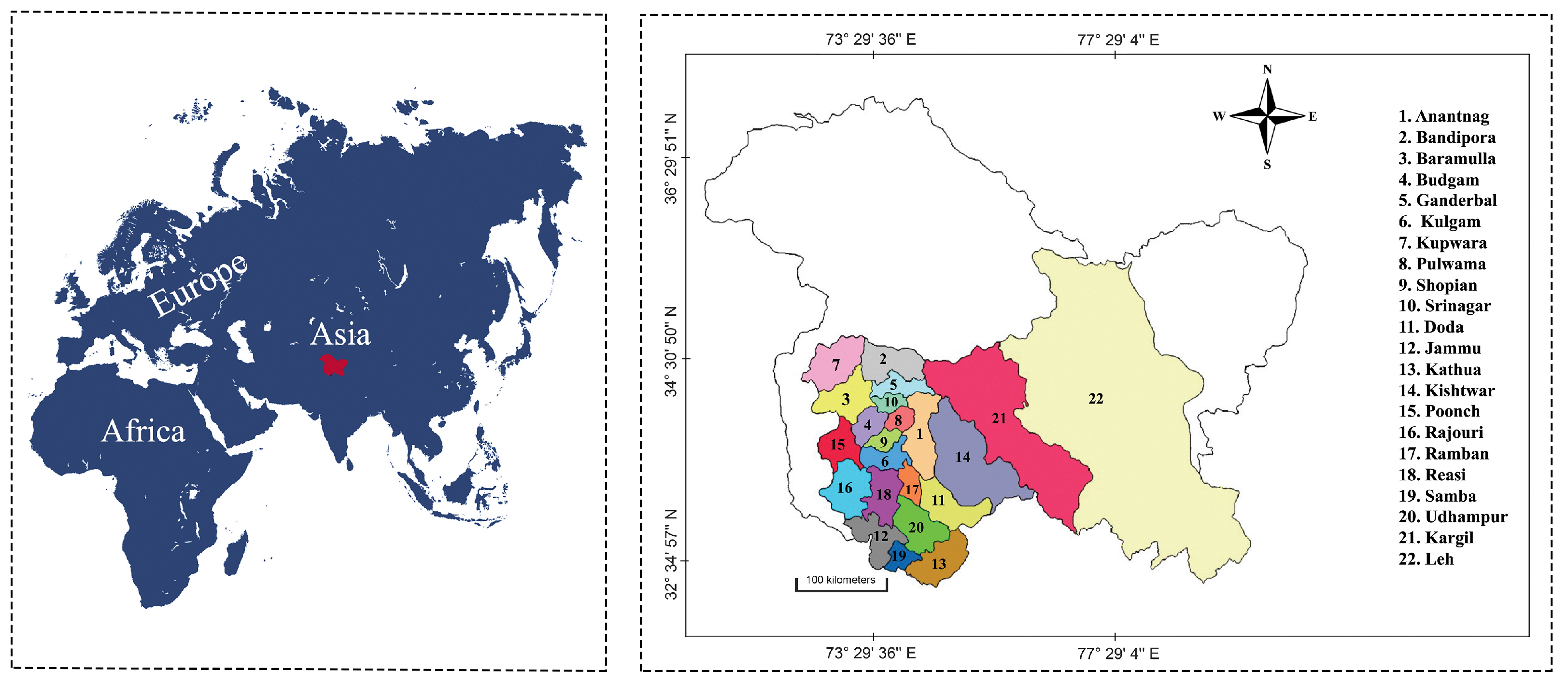
The present study intends to investigate the characteristics of agricultural growth in relationship with various intrinsic/extrinsic variables and assess the vulnerability of agriculture to climatic change in the region of Jammu, Kashmir, and Ladakh. This study area is situated in the northwestern portion of the Himalayan mountain range, characterised by significant variations in terrain elevation, snow-covered peaks, river systems, intricate geological formations, and diverse temperate plant and animal life. The studied area is centrally proximal to three climatic systems of Asia. The region of Punjab, characterised by a weak monsoon zone, is located in its southern border. It is bordered by the vast arid plateau of Tibet in its northeast. In contrast, the northwest border areas face the eastern limits of the Mediterranean climate. Two-thirds (2.3 million ha) of the total mountainous area of India (3.5 million ha) is found in this region. This region lies in the extreme north of the Himalayas. It constitutes about 67.5% of the northwest Himalayan region. There is diversity in the region’s agro-climatic conditions, ranging from temperate in Kashmir, cold arid in Ladakh, and sub-tropical in Jammu. However, the shift in micro-climatic scenarios varies widely across the whole area. A geographical outline of the area under study spans on a net area of about 101,387 km segregated into 22 sub-regions/districts (as shown in Figure 1).
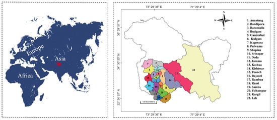
Figure 1.
Continental level position of the studied area highlighted in red (Left): map of the studied area (right).
Table 1 specifies the global location of the districts in the studied area.

Table 1.
Global coordinates of the districts in the studied region.
3.2. Data: Collection, Preprocessing, and Reference Period
This study is based on benchmark secondary data procured from two sources: (1) published records of the Digest of Statistics (Government of Jammu and Kashmir); and (2) NASA LaRC POWER. The data in Table 2 illustrate the exposure, sensitivity, and adaptive capacity variables used in this study for the vulnerability assessment. Table 3 describes the socio-economic indicators that are used in this study for estimating agricultural growth in the presence of these variables. The reference period of study for climatic variables (exposure) spans the years 1983–2022, while the data pertaining to sensitivity and adaptative capacity indicators span from 2007 to 2020. The procured climate data are sampled daily, which was processed to obtain the annual figures as follows:

Table 2.
Various vulnerability indicators categorized into components of exposure, sensitivity, and adaptive capacity along with their positive (+) or negative (−) functional relationship with vulnerability.

Table 3.
Socio-economic and climatic variables considered for the assessment of agricultural growth.
and represent the overall annual maximum and the minimum temperatures in a certain year. The daily data for average temperature and relative humidity on a certain day were averaged to obtain the annual mean figure, and , respectively. The daily precipitation data were summed up to form its annual figure. Equations (1)–(5) detail the process of obtaining the annual data of the mentioned variables.
where , , , , and denote the maximum temperature, minimum temperature, average temperature, relative humidity, and precipitation, respectively, on the ith day of the year (with n days). The annual data for variables , , , and (as defined in Table 2) is derived from , , , and , respectively. The other derived variables, , , and (as defined in Table 3), are derived from , , and , respectively. For all other sensitive, socio-economic, and adaptive capacity variables (as defined in Table 2 and Table 3), the data source exists in annual representation, as it is.
3.3. Vulnerability Assessment: Categorisation of Districts and Indexing of Districts
In this study, a hypothesis for the functional relationship between the vulnerability components and indicators (from Table 2) was established. District-wise vulnerability assessment is performed as an indexing-based standardization approach to categorize various regions on the basis of their relative rank derived from the functional hypothesis. The influence of each variable was captured with an assumption that each variable has a weight equal to that of the overall vulnerability to climate change.
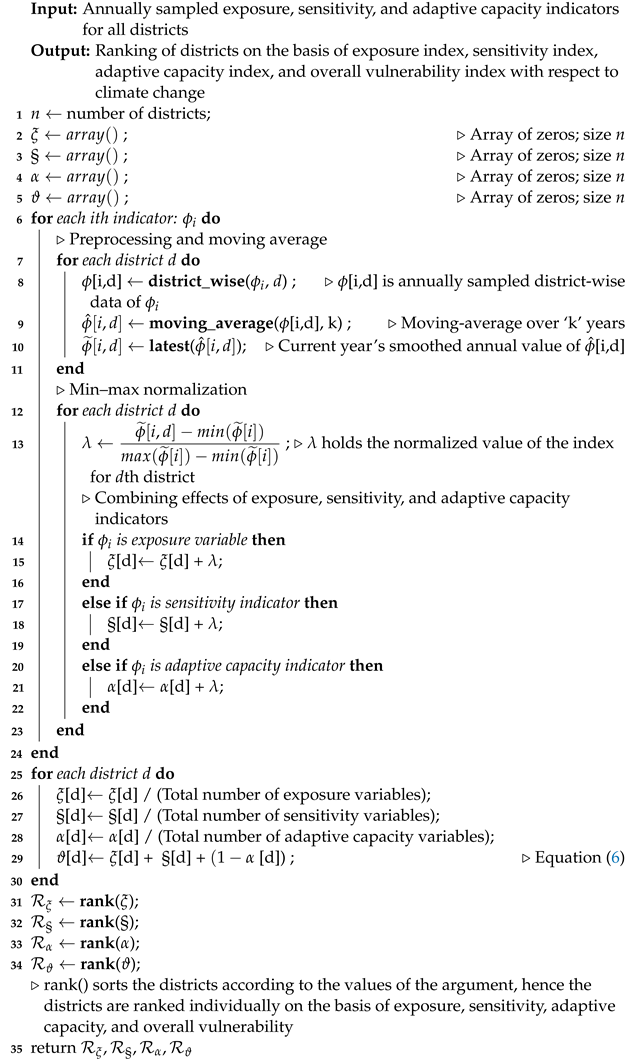
Algorithm 1 illustrates the methodology (pseudo-code) followed in pursuing this objective. Initially, all the annually sampled indicators (), given in Table 2 and Table 3 (except the derived indicators) are treated for the removal of noise, that could be present because of inter-year fluctuations, using the moving-average method on previous k years across all districts. Similarly outliers and missing values are adjusted using standard Gaussian filtering [71]. Then, the current smoothened value of the ith indicator is taken as a reference value of the respective indicator which is again retained for each of the districts. This is followed by the min–max normalization for determining the scaled value of the reference indicator among d districts, denoted by as . Given that the overall performance of a district is quantified separately as indices of exposure (), sensitivity (§), and adaptive capacity (), the relative rank of the dth district among each indicator category is observed as a ranking of averaged , given as , , and each where n is the number of identified districts (in Table 1). Hence, the vulnerability index () of a district is formulated as defined in Equation (6).
| Algorithm 1: Methodology for ranking districts on the basis of vulnerability to climate change. |
 |
3.4. Estimation of the Impact of Climate Change on Agricultural Growth
This study employed the Ricardian method developed by [72] with few modifications to capture the impact of climate change on agricultural growth. This analysis is based on the assumption of a direct cause-and-effect relationship between climate events and agricultural growth. As a modification of the Ricardian method to assess the contribution of environmental conditions towards agricultural growth, the estimated parameter of agricultural growth is taken as a proxy of land rent value (as defined by the original Ricardian model). A modelling function is employed to analyse the impact of different variables on agricultural growth in the presence of climatic variables. Several variables were attempted while estimating the function; however, certain variables (mentioned in Table 3) were retained in their final form. The model of the structural form, as defined in Equation (7), is estimated to give the best fit for the trend of agricultural growth () as a linear combination of the aforementioned variables:
where is a random bias term and () represents the respective coefficients of the variables. The parameters () of the function are estimated using ordinary least squares (OLS)-based linear regression. Prior to performing an analysis of this function, necessary requirements of the linear regression were tested for the purpose of verifying the distributional characteristics in the data. The results of these tests are specified in Appendix A.
3.5. Estimation of Climate Variability and Forecasting
The climatic data variables have temporal characteristics, and it is imperative to model the distribution of such data using recurrent neural networks that have found applications in numerous use-cases. This study leverages a standard long short-term memory [73] (LSTM)-based neural network model to approximate a function on the distribution of climate variables. Although many climatic variables could be compositely taken under consideration, this study mainly focuses on the exposure of climate variability and its impact within agricultural framework, hence the climatic variables under consideration are , , , , . Understanding the distribution system of these climate variables could provide a detailed analysis of the stability of agricultural systems in the current scenario.
Now, the climate variables represent individual time-series signals with distinct temporal distribution. LSTM model is viable for capturing such temporal features having long-range dependencies. Initially, the dataset is treated with standard scaling to mitigate inter-year fluctuations, the removal of noise, and fasten the convergence of the applied model. Standard scaling is applied on each climate variable using the formulation in Equation (8).
where , and represent the mean and standard deviation of , respectively. The motivation to utilize the neural network approach for the objective of forecasting climate variables has three reasons: firstly, the universal approximation theorem suggests that neural networks are an excellent choice for modelling continuous functions [74]. This is true, irrespective of the possible trends, oscillations, seasonality or other properties in the data. Secondly, LSTM [73] neural networks have the tendency to capture temporal characteristics in the data samples that have long-range dependencies, on previous values, across time. The climate data distribution is expected to follow a Markov chain [75], and may not be stationary (such as in the case of temperature or precipitation). Furthermore, some climate variables do not follow a linear trend of expectation, and some can experience change in variances with time (such as precipitation and relative humidity). Hence, most climate data cannot be generalized well by linear econometric models (unless some additional processing is performed, such as when the first-order differences of the time series are modelled using these models instead of actual data). Thirdly, non-linear parametric econometric models [76,77,78] tend to assume the parameters of the model according to the statistical properties of the data, prior to modelling, which could fail in predicting uneven/sudden changes in the data (such as predicting erratic precipitation). The parameters are tuned according to the statistical characteristics found in the data prior to achieving the generalization. In contrast, the parameters of the neural network-based predictors are tuned as a process during its training phase by some suitable learning algorithms (such as SGD [79]). In the latter case, there is no need to manually re-engineer the parameters of the model or assume the statistical properties in the data (such as stationarity, scedasticity, or type of probability distribution); hence, there is the potential to achieve better generalization.
Now, some climate variables in the dataset could be correlated and some are apparent to be completely uncorrelated. To remove any hazard that could occur due to inter-variable dependency towards model convergence, an individual LSTM-based neural network is trained for each climate variable. This helps understand the trend of each variable discretely. Secondly, the agricultural systems tend to be complicated across geography. For instance, crops across regions can have distinct dependence on a specific subset or, sometimes, all of climate variables. It is thus essential to consider approximating the distributions of the climate variables in separation from one another for the objectives of forecasting. The scaled transformation of the data of each climate indicator is modelled using the proposed model (as illustrated in Figure 2). The input to the LSTM layer is first resampled into features which specifies the network to use m previous annual values to predict one futuristic estimate of the input variable. Hence, the series of 39 annually sampled values for each district is featured in the form of samples (each of length of m units) in each variable of each district. The defined LSTM layer has four cells. Consider the sequence as input to the LSTM cell at any time t which is transformed across its different gates [80] using the formulation (as shown in Equations (9)–(14)).
where represents the trainable parameters of the LSTM baseline. The output vector from the LSTM cell is forwarded (after 60% dropout) as input to two dense layers ( and ), each with ten nodes. The output is forwarded to a ReLU activation layer to yield a normalized prediction value (y) as shown in Equation (15). and represent the trainable parameters of the fully connected layers.

Figure 2.
Proposed LSTM-based model for modelling climate variability.
Then, a procedural inverse standard scalar processes the overall output to yield a futuristic estimate of the sample. We repeat the training procedure for multiple epochs until an apparent convergence of the model is reached. It is essential to realize that, even though LSTMs are capable of approximating data that are frequently sampled (such as daily or monthly), it is appropriate to generate year-long average predictions rather than generating for more frequent periods because of the following reason: climate change is observable for sufficiently long periods of time. Frequently sampled data tend to be more stochastic than otherwise. In this context, capturing stochasticity, something LSTMs would be capable of, is not the purpose. The purpose is to visualize year-long or decade-long projections. In this case, neural networks trained for more frequently sampled data would yield more error when generating such longer projections because they would expect stochastic behaviour to exist in yearly sampled data as well. To prevent the model to overfit, we limit the LSTM cells to be only four in comparison to the number of training samples in each variable. In addition, we add significant dropout rate to prevent any uncontrolled overfitting.
4. Results and Discussion
This section details the results observed and the corresponding experimental analysis of the objectives.
4.1. Estimation of Climate Variability and Forecasting
The set of initial settings and hyper-parameter space assumed during the training phase of the proposed LSTM-based framework for forecasting climate variables are illustrated in Table 4.

Table 4.
Hyper-parameter space of proposed deep-learning-based architecture for the analysis and forecasting of climate data.
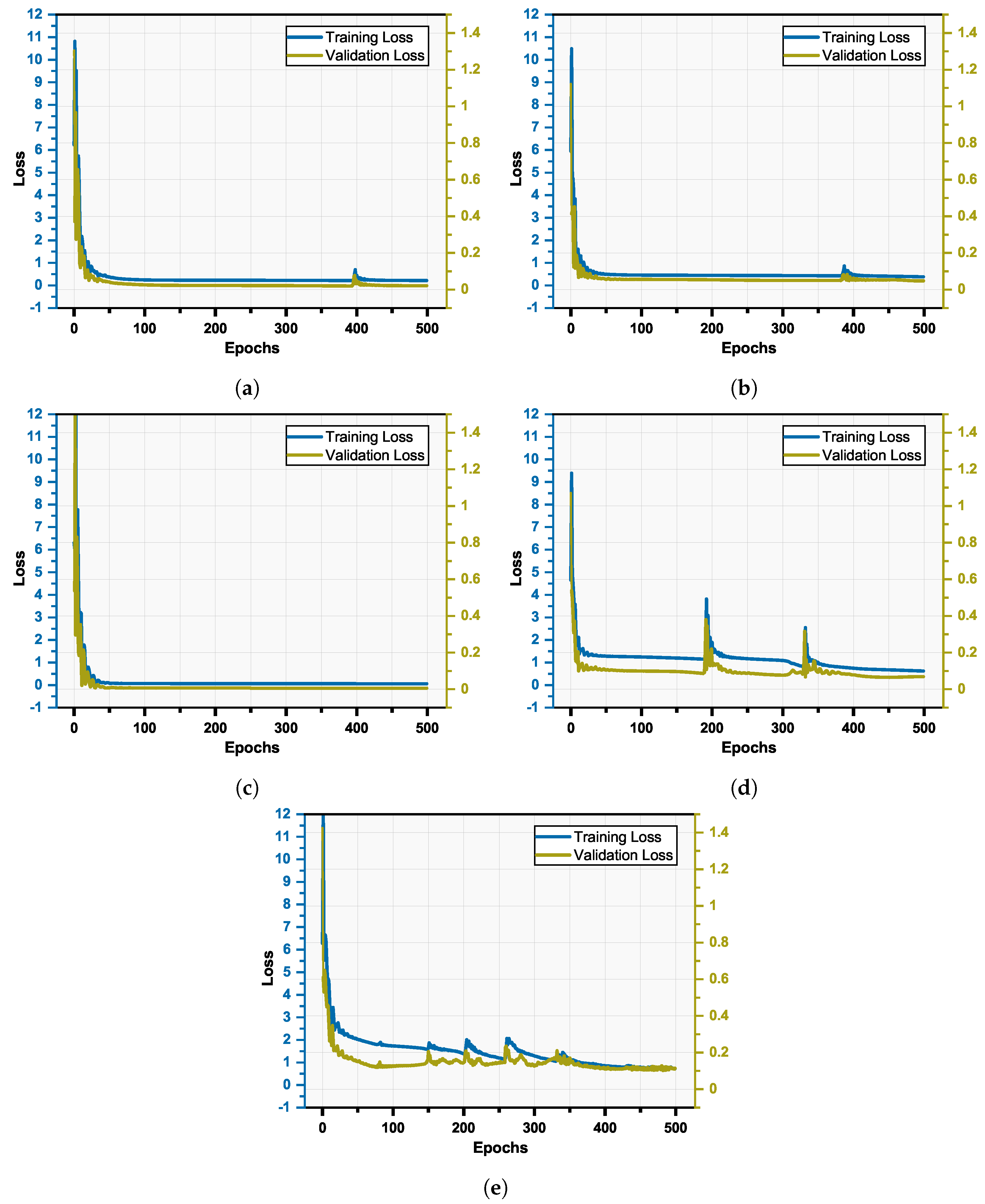
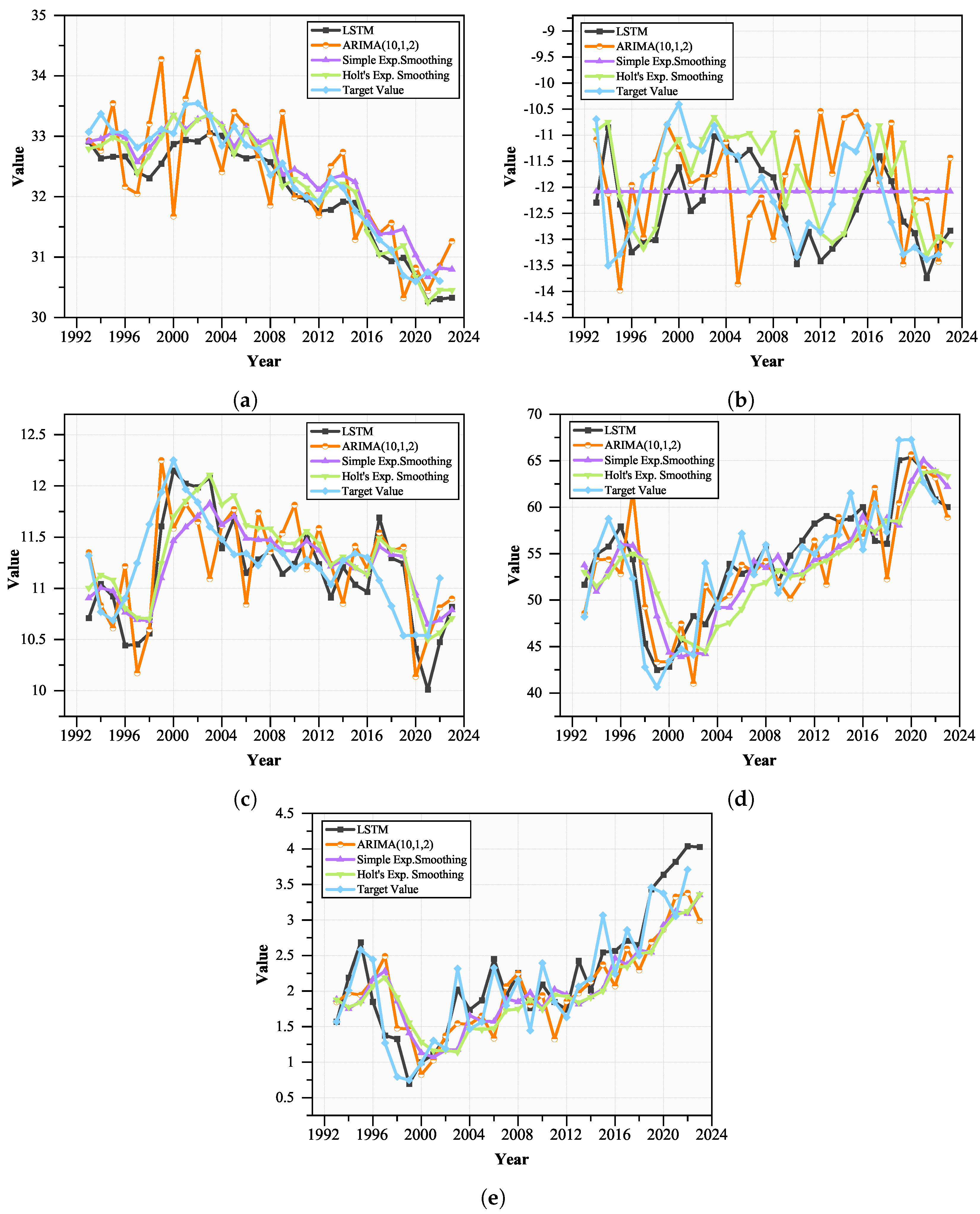
Initially, the data corresponding to each district comprise 39 years’ worth of annually sampled data for each of five climate variables. The size of training window is and the stride length is , yielding feature vectors in each district in each variable, each of which is 10 units long. There are a total of 22 districts under study. Hence, the dimensions of feature vectors across all districts in each variable are 638 × 10. The ratio of splitting training data, validation data, and test data was kept as 0.8:0.1:0.1 with the dimensions of 528 × 10, 66 × 10, 66 × 10 samples, respectively. The model is trained for 500 epochs and the learning algorithm is set with Adam optimization for faster convergence. Each input sample is in the dimension specifying the previous 10 annual values used to predict one futuristic estimate with a unit sliding window stride. Five different neural networks are thus trained for the five specified climate variables. The overall loss and convergence patterns of each network are illustrated in Figure 3a–e. The overall mean squared error (on normalized validation data) figures achieved on the proposed network for , , , , and variables are 0.0211, 0.0483, 0.0057, 0.0695, and 0.1022, respectively. Since the generated predictions are conditional on the first 10 annual values of each variable, the predictions are generated by the neural network model from the year 1993 onward, until the year 2023. We proceed to provide a comparative analysis of the proposed LSTM-framework for forecasting the climate variables with respect to some benchmark econometric models (illustrated in Table 5) in terms of root mean squared error (RMSE) and mean absolute error (MAE). We perform forecasting against the actual unnormalized target values from 1993 to 2023 (including unnormalized train, test, and validation data) across all the compared models, viz., LSTM, ARIMA(10,1,2) [76], simple exponential smoothing [77] and Holt’s exponential smoothing [78] (smoothing parameters of 0.3 and 0.5). Figure 4a–e showcase the variability patters and corresponding predictions generated from the compared models in the region for each of the climate variables.
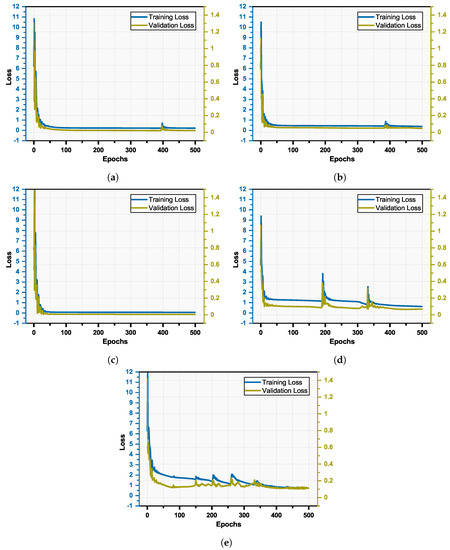
Figure 3.
Loss plot of proposed LSTM−based network for studied climate variables. (a) (b) (c) (d) (e) .

Table 5.
Comparative tabulation of root mean squared error (RMSE) and mean absolute error (MAE) between predicted values and target values in each model.
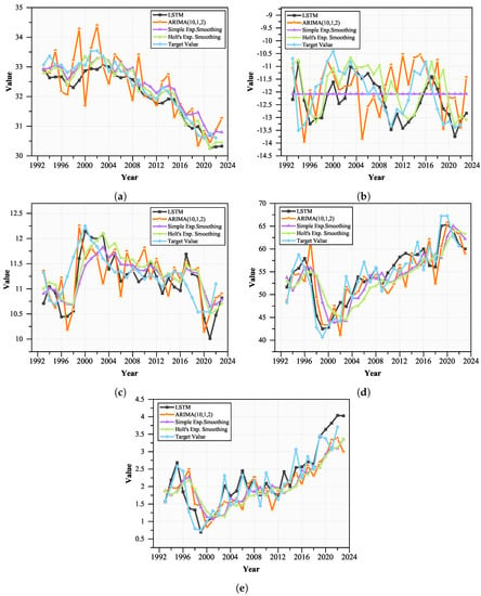
Figure 4.
Variability and forecasting for studied climate variables. (a) (b) (c) (d) (e) .
As can be seen from the results, the proposed LSTM-based architecture achieves a considerable convergence and acceptable error. As seen from Figure 3a–e, the training loss and validation loss almost coincide at convergence, suggesting that the LSTM-approximator has a better fit to the distribution of climate data with respect to the compared models (as shown in Table 5). We proceed to analyse the climate variability using the specified neural network model by generating estimations of futuristic annual figures for all climate variables averaged across districts.
4.2. Analysis of Exposure of the Studied Region to Climate Change
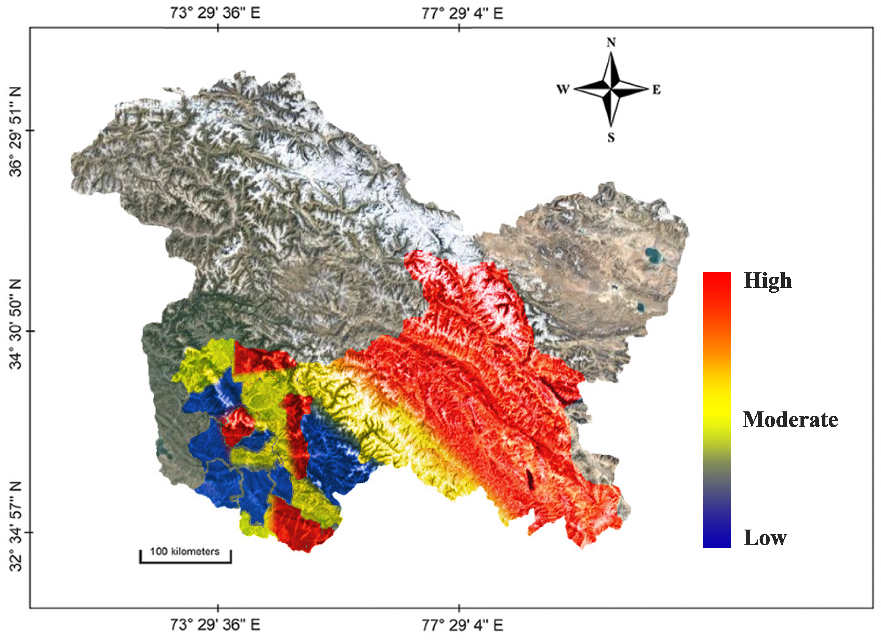
As reported from the results, an overall decrease in the annual maximum temperature () is observed during the period 1993–2023. It is worth noting that does not represent an averaged number but a distribution of annually observed maximal temperature values. Significant impacts are seen in and . is observed to have a normal distribution during the years 1993–2023 with a deviation of about 1.05–1.28 C, and is observed to have an increasing trend. A similar observation was seen in [81]. On the other hand, representing the average temperature is showing an increasing trend from 1993 of about 0.8–1 C with a variance of . It is seen that the trends of annual relative humidity () and annual precipitation () are increasing rapidly [82]. The repercussions of a collective system of these interacting variables can have diverse effects on the cropping framework across the spectrum. The extent of exposure is seen to vary across districts in the studied region. A heatmap representation of the studied region is shown in Figure 5 which illustrates the exposure in the studied region.

Figure 5.
Heatmap showing the exposure to climate change in the studied region across various districts.
4.3. Analysis of Sensitivity to Climate Change
Due to commercialisation and urbanisation, land holdings () have shrunk across the region. On such terrain, basic agricultural activities are undesirable, and it renders stakeholders susceptible to climate change. The average landholding has been decreasing over the years, exhibiting a ha difference since 1983. The magnitude of sensitivity of an area is directly proportional to its area under culturable waste lands (), and it is reported to show a decreasing trend. The premise of increasing freshwater scarcity [83] poses a threat to the populace that depends on water-demanding food crops (such as rice [84]). The quantity of the area utilized for such an agricultural product along with the associated population are, thus, susceptible. In the extension to this context, any long-term change in climate would impress an impact on the hydrological regimes of an area with consequent effects on its irrigation system, making water-dependent crops even more sensitive. We witnessed an increase in the gross irrigated area () and net irrigated area () with district Leh having the largest area under its influence. We also observed that the principal food crops in Jammu and Kashmir followed a decreasing trend since 1983. Rice acreage is declining due to the large-scale conversion of the area into commercial, residential, and horticultural fields (particularly apple orchards). Although the irrigation system of apple is less complex, meeting the requirements of sufficient chilling hours is essential for its sustainability. A long-term increase in threatens apple production. We proceed to quantify the illiteracy rate () as a parameter of sensitivity because it poses a hurdle in establishing mitigation measures and promoting awareness. Since the districts of Jammu, Kashmir and Ladakh largely qualify as socially suburban, all of the districts have average illiteracy rates (with district Budgam reporting the highest illiteracy rate). Illiteracy is also an indirect indicator of unemployment and poverty scenario in the district. Owing to all these factors, climate stress affects the populace that entirely depends on its agricultural footprint. However, we report a declining percentage of agricultural workers () but an increasing percentage of agricultural labourers (), with the highest percentage increase in district Kargil. Lastly, we analyse the role of population characteristics with the objective of specifying the sensitivity of the area. In densely populated areas, the distribution and availability of natural resources such as water, food, and energy become more challenging. Dense populations are more susceptible to the spread of climate-related diseases. In addition, social vulnerability can be higher in densely populated areas, as these communities often face challenges in accessing resources, services, and timely emergency response during climatic catastrophes. A region’s sensitivity is also measured in terms of its BPL population (), both are positively correlated because of lower access to strategic resources. It was observed that the Srinagar district, followed by Bandipora, has the highest population density () while district Leh has the least. In this framework, Figure 6 illustrates a heatmap representation of the studied area to quantify its district-wise sensitivity to climate variability.

Figure 6.
Heatmap showing the sensitivity to climate change in the studied region across various districts.
4.4. Analysis of Adaptation to Climate Change
The adaptive capacity of a system relies on various socio-economic elements, including the progress of infrastructure, availability of essential resources, and span of literacy. Infrastructure development indicators, such as health and educational facilities, as well as road density, play a significant role in determining the adaptation backbone of a region. Access to technology, electrification, percentage of the female workforce, infrastructural/institutional development, and literacy rate are its other essential indicators. Here, we proceed to discuss the trends of significant adaptive capacity indicators. An analysis of data in our study revealed a rise in regional cropping intensity () [85] and irrigation intensity () across all districts. Similarly, we saw an increase in the net sown area () in various districts. An increase in livestock productivity is another positive indication of the adaptive capacity. Since ancient times, livestock and their products have supplemented crop production, provided means of sustenance during lean seasons, and improved resilience to climatic extremes [86]. Livestock productivity increases with the increase in fodder crops () and it was observed that Kargil has the highest percentage of land under fodder crops, Udhampur the lowest, while many districts lag behind this benchmark. On the other hand, the districts in the Kashmir sub-region saw a slight decrease in forest cover, which is otherwise effective in managing the micro-climate settings. This behaviour is attributed to the rapid exploitation of the natural habitat. We have taken the area under walnut () as an adaption measure as these are robust fruit crops that may survive adverse weather conditions and reduce financial stress in the failure of field crops. Its cultivation has expanded due to public understanding of its benefits (with Kishtwar leading the spectrum). In the next context, the noticeable increase in literacy rates could help bring about preparation for and awareness of the impacts of climate change and help in developing the corresponding mitigation strategies [87]. Similarly, with the reported increase in rural electrification () numbers, farming mechanisation could help in stressed areas by maximising land utilisation. Various other indicators pertinent to housing, infrastructure, and welfare, which help stakeholders in terms of financial stability and risk-coverage, have grown overall in the region. While the trends of all aforementioned indicators have been reported for the overall region, some districts show relatively worse performances. A heatmap representation is shown in Figure 7 that illustrates the relative performance of the adaptive capacity among the districts in the studied region.

Figure 7.
Heatmap showing the adaptive capacity to climate change in the studied region.
4.5. Categorisation of Districts on the Basis of Climate Vulnerability
The vulnerability to climate change reflects an aggregate effect of various exposure, sensitivity, and adaptation parameters [18]. The Leh, Kathua, and Bandipora districts demonstrated the highest variability in the climate variables, especially due to a higher rate of change in precipitation and temperatures. As far as sensitivity variables are concerned, the Budgam, Bandipora, and Ganderbal districts were found to be highly sensitive, mainly due to higher illiteracy rates, population density, area under rice, area under apple, number of agri-labourers, and net irrigated area. On the other hand, the Budgam, Ganderbal, and Pulwama districts were found to be highly adaptive. Based upon the aggregation of exposure, sensitivity, and adaptation variables as defined by Equation 1, the districts Budgam, Bandipora, and Ganderbal were found to be the most vulnerable areas to climate change, while as the Kargil, Rajouri, and Poonch districts were found to be the least vulnerable due to various socio-economic factors and institutional measures. Furthermore, the central part of Kashmir valley was found to be the most vulnerable sub-region, followed by northern Kashmir, and then followed by southern Kashmir. Figure 8 illustrates a heatmap representation of the overall vulnerability pattern in the studied region.
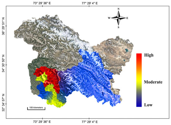
Figure 8.
Heatmap showing the vulnerability to climate change in the studied region across various districts.
4.6. Impact of Climate Change and Agricultural Growth Model
An ordinary least squares-based estimation scheme was employed to determine the coefficients of indicator variables (discussed in Equation (7)). Table 6 summarises the estimates of these coefficients used in modelling agricultural growth [88] as a linear regression function. The estimates of these coefficients help us realize the correlation of the indicators with respect to agricultural growth. The variability in climate variables was seen to have a serious negative influence on the agricultural growth modelled as a Ricardian function (Equation (7)). The decreasing land holdings also show a significant negative impact on the growth. The determinant factor of this result is attributed to the increase in annual minimum temperature (). The number of inputs, technology, and institutional variables, including the public investment in agriculture, have significantly contributed towards positive agricultural growth. The rural literacy rate was also found to be one of the important variables, influencing agricultural growth, in a positive direction. These findings advocate a holistic approach to reducing the negative influence of climate change and impart resilience in the production system of the region.

Table 6.
Estimates of the coefficients pertinent to the agricultural growth model defined in Equation (7).
5. Conclusions
This study conducted an empirical investigation in the region of Jammu, Kashmir, and Ladakh with the aim of assessing its agricultural growth, modelled as a linear regression function under the influence of the variables of climatic stress and socio-economic indicators. The estimated coefficients detail the underlying dependence of agricultural performance on various variables that could help in establishing proactive/mitigation strategies in the agricultural paradigm against climate variability. We propose a framework for quantifying the vulnerability of twenty-two sub-regions (districts) of the studied region utilizing min–max normalization-based ranking scheme that helps to identify the underlying hazardous indicators in a region and its subsequent resilience factors. The sub-regions were categorised according to the indexed values that provide an understanding of the causes and prospective adaptive policies towards the threat of climate variability. An analysis of trends in climate variability was performed with the comprehensive detailing of region-level effects, using an LSTM-backbone model. Our proposed approach yields significant accuracy in predicting the annual estimate of five climate variables that have a direct relationship with the agricultural footprint in the region. Our work provides a baseline for all prospective studies towards the quantification of the region’s susceptibility to climate change.
Author Contributions
Conceptualization, I.M., M.A., Y.G., S.H.B., M.S.M. and A.B.S.; Data curation, I.M., M.A., Y.G. and S.H.B.; Formal analysis, I.M., M.A. and Y.G.; Funding acquisition, Y.G.; Investigation, I.M., M.A., Y.G. and A.S.; Methodology, I.M., M.A., Y.G. and M.S.M.; Project administration, Y.G.; Resources, I.M., M.A. and Y.G.; Software, I.M., M.A., Y.G. and S.H.B.; Supervision, Y.G., M.S.M. and A.S.; Validation, I.M., M.A., Y.G. and S.H.B.; Visualization, Y.G. and O.E.; Writing—original draft, I.M., M.A. and Y.G.; Writing—review and editing, Y.G., S.H.B., M.S.M., A.B.S., A.S. and O.E. All authors have read and agreed to the published version of the manuscript.
Funding
This work was supported by the Deanship of Scientific Research, Vice Presidency for Graduate Studies and Scientific Research, King Faisal University, Saudi Arabia, under Project Grant 3,672.
Institutional Review Board Statement
Not applicable.
Informed Consent Statement
Not applicable.
Data Availability Statement
The data used in this study were curated from the datasets of Digest of Statistics—Government of Jammu and Kashmir [37]; and NASA LaRC POWER [38]. The data are publicly available and can be obtained from the mentioned sources.
Conflicts of Interest
The authors declare no conflict of interest.
Appendix A
Whilst undertaking the third objective of this study, which pertains to modelling the agricultural growth function as a linear combination of socio-economic and derived exposure variables (as defined in Equation (7)), some diagnostic tests were performed on the framed model comprising the empirically selected set of variables, determining whether a linear estimator could be considered for modelling this function. The results of the tests were discussed in the following subsections:
Appendix A.1. Test of Auto-Correlation of Residuals (Durbin–Watson Test)
We leverage the Durbin–Watson statistic () to test the presence or absence of auto-correlation in the residuals, defined as , where is a parameter of the function, and denote the observed and predicted values of the response variable, denotes sample auto-correlation, and . Considering the null hypothesis () that residuals are auto-correlated, while the residuals are not auto-correlated in the alternative hypothesis (), the Durbin–Watson statistic recorded the value of 2.09 (very close to 2), accepting the alternative hypothesis. The observed statistic indicates that there was no significant correlation among the residuals, which can thus be treated as independent.
We proceed to extend the deduction using Ljung–Box auto-correlation test, against the same set of hypotheses. The statistics and p-values in across lags = {1, 2, 3, …, 30} are illustrated in Table A1. Since the p-value > 0.05, then the null hypothesis is accepted.

Table A1.
Results of Ljung–Box auto-correlation test.
Table A1.
Results of Ljung–Box auto-correlation test.
| Ljung–Box (LB) Test | ||||||
|---|---|---|---|---|---|---|
| Lag-value | 1 | 2 | 3 | 4 | 5 | 6 |
| LB statistic | 2.013155 | 2.03636 | 5.550541 | 7.324725 | 7.352519 | 7.353024 |
| LB p-value | 0.155941 | 0.361252 | 0.135647 | 0.119691 | 0.195715 | 0.289429 |
| Lag-value | 7 | 8 | 9 | 10 | 11 | 12 |
| LB statistic | 10.32041 | 10.99063 | 11.23732 | 11.26712 | 12.70028 | 12.88068 |
| LB p-value | 0.171132 | 0.202231 | 0.259792 | 0.337089 | 0.313365 | 0.377773 |
| Lag-value | 13 | 14 | 15 | 16 | 17 | 18 |
| LB statistic | 13.76404 | 14.81549 | 16.67063 | 16.67072 | 16.72562 | 17.02409 |
| LB p-value | 0.390669 | 0.390883 | 0.338932 | 0.407208 | 0.4731 | 0.521449 |
| Lag-value | 19 | 20 | 21 | 22 | 23 | 24 |
| LB statistic | 17.1546 | 17.17511 | 17.5885 | 18.89323 | 18.89363 | 18.94258 |
| LB p-value | 0.579395 | 0.641575 | 0.674875 | 0.651912 | 0.707381 | 0.755045 |
| Lag-value | 25 | 26 | 27 | 28 | 29 | 30 |
| LB Statistic | 20.37629 | 20.54265 | 21.74614 | 22.27702 | 24.35248 | 27.60363 |
| LB p-value | 0.726819 | 0.765169 | 0.750163 | 0.768308 | 0.711367 | 0.591433 |
Appendix A.2. Test of Collinearity (Variance–Inflation Factor Statistic)
The variance–inflation factor () is used to measure the extent to which the variance of the estimated regression coefficient is increased due to collinearity. The results are tabulated in Table A2.

Table A2.
Variance–inflation factor test results.
Table A2.
Variance–inflation factor test results.
| Indicator | Tolerance | Indicator | Tolerance | ||
|---|---|---|---|---|---|
| 0.351 | 2.845 | 0.271 | 3.687 | ||
| 0.977 | 1.023 | 0.665 | 1.503 | ||
| 0.209 | 4.782 | 0.317 | 3.149 | ||
| 0.189 | 5.277 | 0.488 | 2.047 | ||
| 0.242 | 4.126 | 0.205 | 4.87 | ||
| 0.234 | 4.268 | 0.209 | 4.784 | ||
| 0.312 | 3.197 | 0.426 | 2.343 |
values above indicate the presence of collinearity, with higher values suggesting stronger collinearity. Typically, values above 5–6 are considered indicative of a higher degree of collinearity and as per the results the values (and the corresponding tolerance) are in the justifiable range that showed a minor spectrum of multicollinearity between variables.
Appendix A.3. Test of Normality (Shapiro–Wilk Statistic)
We test the null hypothesis () against an alternative hypothesis () defined as
: residuals are normally distributed.
: residuals are not normally distributed.
The required test statistic () is defined as
where k = , when n is even and k = , otherwise. The distribution from denotes the sorted values of the sample distribution (). The values of are compared to the benchmark threshold values () at significance level () framed in [89]. If the calculated value of is less than , then is rejected, or otherwise accepted. The parameters of the statistic are illustrated in Table A3.

Table A3.
Results of Shapiro–Wilk test to check normality of residuals.
Table A3.
Results of Shapiro–Wilk test to check normality of residuals.
| Indicator | p-Value | Significance | |
|---|---|---|---|
| 0.763 | 0.231 | NS | |
| 0.952 | 0.166 | NS | |
| 0.925 | 0.069 | NS | |
| 0.878 | 0.072 | NS | |
| 0.921 | 0.082 | NS | |
| 0.951 | 0.152 | NS | |
| 0.925 | 0.079 | NS | |
| 0.944 | 0.096 | NS | |
| 0.822 | 0.100 | NS | |
| 0.963 | 0.326 | NS | |
| 0.979 | 0.763 | NS | |
| 0.983 | 0.875 | NS | |
| 0.982 | 0.861 | NS | |
| 0.944 | 0.098 | NS | |
| 0.923 | 0.065 | NS |
NS denotes non-significant.
Shapiro–Wilk test statistic was found to be non-significant (p-Value > 0.05) at 5% level significance, indicating that the assumptions of the randomness and normal distribution of the residuals were satisfied.
Appendix A.4. Test of Homoscedasticity: White Test and Breusch–Pagan–Godfrey Test
To verify the presence of homoscedasticity in the residuals, we test the null hypothesis () against the alternative hypothesis () defined as
: homoscedasticity is present.
: heteroscedasticity is present.
To concede to the appropriate hypothesis, we undertake the White test and Breusch–Pagan–Godfrey test, the results of which are specified in Table A4.

Table A4.
Results of the White test and the Breusch–Pagan–Godfrey Test.
Table A4.
Results of the White test and the Breusch–Pagan–Godfrey Test.
| White Test | Breusch–Pagan–Godfrey Test | ||
|---|---|---|---|
| Test statistic | 7.0766 | Lagrange multiplier statistic | 7.9956 |
| Test statistic p-value | 0.2150 | p-value | 0.8895 |
| F-statistic | 1.4764 | F-statistic | 0.4044 |
| F-statistic p-value | 0.2314 | F-statistic p-value | 0.9532 |
For the White test analysis, since the p-value > 0.05, we accept the null hypothesis. The same conclusion was obtained for the Breusch–Pagan–Godfrey test, hence it is conceded that the residuals are homoscedastic.
References
- Bernstein, L.; Bosch, P.; Canziani, O.; Chen, Z.; Christ, R.; Riahi, K. 2007: Climate Change 2007: Synthesis Report; IPCC: Geneva, Switzerland, 2008. [Google Scholar]
- Staudt, A.; Leidner, A.K.; Howard, J.; Brauman, K.A.; Dukes, J.S.; Hansen, L.J.; Paukert, C.; Sabo, J.; Solórzano, L.A. The added complications of climate change: Understanding and managing biodiversity and ecosystems. Front. Ecol. Environ. 2013, 11, 494–501. [Google Scholar] [CrossRef]
- Maure, D.; Kittel, C.; Lambin, C.; Delhasse, A.; Fettweis, X. Spatially heterogeneous effect of the climate warming on the Arctic land ice. Cryosphere Discuss. 2023, 2023, 1–20. [Google Scholar]
- Arnell, N.W.; Lowe, J.A.; Challinor, A.J.; Osborn, T.J. Global and regional impacts of climate change at different levels of global temperature increase. Clim. Chang. 2019, 155, 377–391. [Google Scholar] [CrossRef]
- Altizer, S.; Ostfeld, R.S.; Johnson, P.T.; Kutz, S.; Harvell, C.D. Climate change and infectious diseases: From evidence to a predictive framework. Science 2013, 341, 514–519. [Google Scholar] [CrossRef] [PubMed]
- Berrang-Ford, L.; Siders, A.; Lesnikowski, A.; Fischer, A.P.; Callaghan, M.W.; Haddaway, N.R.; Mach, K.J.; Araos, M.; Shah, M.A.R.; Wannewitz, M.; et al. A systematic global stocktake of evidence on human adaptation to climate change. Nat. Clim. Chang. 2021, 11, 989–1000. [Google Scholar] [CrossRef]
- Zhang, J.; Shi, K.; Paerl, H.W.; Rühland, K.M.; Yuan, Y.; Wang, R.; Chen, J.; Ge, M.; Zheng, L.; Zhang, Z.; et al. Ancient DNA reveals potentially toxic cyanobacteria increasing with climate change. Water Res. 2023, 229, 119435. [Google Scholar] [CrossRef] [PubMed]
- Adediran, I.A.; Isah, K.O.; Ogbonna, A.E.; Badmus, S.K. A global analysis of the macroeconomic effects of climate change. Asian Econ. Lett. 2023, 4. [Google Scholar] [CrossRef]
- Jha, B.; Tripathi, A. How susceptible Is India’s food basket to climate change? Soc. Chang. 2017, 47, 11–27. [Google Scholar] [CrossRef]
- Bhattacharyya, P.; Pathak, H.; Pal, S.; Bhattacharyya, P.; Pathak, H.; Pal, S. Impact of climate change on agriculture: Evidence and predictions. Clim. Smart Agric. Concepts Chall. Oppor. 2020, 17–32. [Google Scholar]
- World Bank. World Bank Open Data; World Bank: Washington, DC, USA, 2020. [Google Scholar]
- Easterling, W.E.; Aggarwal, P.K.; Batima, P.; Brander, K.M.; Erda, L.; Howden, S.M.; Kirilenko, A.; Morton, J.; Soussana, J.F.; Schmidhuber, J.; et al. Food, fibre and forest products. Clim. Chang. 2007, 2007, 273–313. [Google Scholar]
- Raza, A.; Razzaq, A.; Mehmood, S.S.; Zou, X.; Zhang, X.; Lv, Y.; Xu, J. Impact of climate change on crops adaptation and strategies to tackle its outcome: A review. Plants 2019, 8, 34. [Google Scholar] [CrossRef]
- Kumar, R.; Gautam, H.R. Climate change and its impact on agricultural productivity in India. J. Climatol. Weather. Forecast. 2014, 2, 1–3. [Google Scholar] [CrossRef]
- Malhi, G.S.; Kaur, M.; Kaushik, P. Impact of climate change on agriculture and its mitigation strategies: A review. Sustainability 2021, 13, 1318. [Google Scholar] [CrossRef]
- Akhtar, R.; Masud, M.M. Dynamic linkages between climatic variables and agriculture production in Malaysia: A generalized method of moments approach. Environ. Sci. Pollut. Res. 2022, 29, 41557–41566. [Google Scholar] [CrossRef]
- Jamshidi, O.; Asadi, A.; Kalantari, K.; Azadi, H.; Scheffran, J. Vulnerability to climate change of smallholder farmers in the Hamadan province, Iran. Clim. Risk Manag. 2019, 23, 146–159. [Google Scholar] [CrossRef]
- Fellmann, T. The assessment of climate change-related vulnerability in the agricultural sector: Reviewing conceptual frameworks. Build. Resil. Adapt. Clim. Chang. Agric. Sect. 2012, 23, 37. [Google Scholar]
- Reed, M.; Podesta, G.; Fazey, I.; Geeson, N.; Hessel, R.; Hubacek, K.; Letson, D.; Nainggolan, D.; Prell, C.; Rickenbach, M.; et al. Combining analytical frameworks to assess livelihood vulnerability to climate change and analyse adaptation options. Ecol. Econ. 2013, 94, 66–77. [Google Scholar] [CrossRef]
- IPCC, W. Special report on emissions scenarios. In Intergovernmental Panel on Climate Change Special Reports on Climate Change; Cambridge University Press: Cambridge, UK, 2000; Volume 570. [Google Scholar]
- Anand, V.; Gupta, S.; Gupta, D.; Gulzar, Y.; Xin, Q.; Juneja, S.; Shah, A.; Shaikh, A. Weighted Average Ensemble Deep Learning Model for Stratification of Brain Tumor in MRI Images. Diagnostics 2023, 13, 1320. [Google Scholar] [CrossRef]
- Gulzar, Y.; Khan, S.A. Skin Lesion Segmentation Based on Vision Transformers and Convolutional Neural Networks—A Comparative Study. Appl. Sci. 2022, 12, 5990. [Google Scholar] [CrossRef]
- Khan, S.A.; Gulzar, Y.; Turaev, S.; Peng, Y.S. A modified HSIFT Descriptor for medical image classification of anatomy objects. Symmetry 2021, 13, 1987. [Google Scholar] [CrossRef]
- Alam, S.; Raja, P.; Gulzar, Y. Investigation of Machine Learning Methods for Early Prediction of Neurodevelopmental Disorders in Children. Wirel. Commun. Mob. Comput. 2022, 2022, 5766386. [Google Scholar] [CrossRef]
- Sahlan, F.; Hamidi, F.; Misrat, M.Z.; Adli, M.H.; Wani, S.; Gulzar, Y. Prediction of Mental Health Among University Students. Int. J. Perceptive Cogn. Comput. 2021, 7, 85–91. [Google Scholar]
- Dhanya, V.; Subeesh, A.; Kushwaha, N.; Vishwakarma, D.K.; Kumar, T.N.; Ritika, G.; Singh, A. Deep learning based computer vision approaches for smart agricultural applications. Artif. Intell. Agric. 2022, 6, 211–229. [Google Scholar] [CrossRef]
- Gulzar, Y. Fruit Image Classification Model Based on MobileNetV2 with Deep Transfer Learning Technique. Sustainability 2023, 15, 1906. [Google Scholar] [CrossRef]
- Yang, B.; Xu, Y. Applications of deep-learning approaches in horticultural research: A review. Hortic. Res. 2021, 8, 123. [Google Scholar] [CrossRef]
- Igried, B.; AlZu’bi, S.; Aqel, D.; Mughaid, A.; Ghaith, I.; Abualigah, L. An Intelligent and Precise Agriculture Model in Sustainable Cities Based on Visualized Symptoms. Agriculture 2023, 13, 889. [Google Scholar] [CrossRef]
- Ayoub, S.; Gulzar, Y.; Rustamov, J.; Jabbari, A.; Reegu, F.A.; Turaev, S. Adversarial Approaches to Tackle Imbalanced Data in Machine Learning. Sustainability 2023, 15, 7097. [Google Scholar] [CrossRef]
- Bali, N.; Singla, A. Emerging Trends in Machine Learning to Predict Crop Yield and Study Its Influential Factors: A Survey; Springer: Berlin/Heidelberg, Germany, 2022; pp. 1–18. [Google Scholar]
- Aggarwal, S.; Gupta, S.; Gupta, D.; Gulzar, Y.; Juneja, S.; Alwan, A.A.; Nauman, A. An Artificial Intelligence-Based Stacked Ensemble Approach for Prediction of Protein Subcellular Localization in Confocal Microscopy Images. Sustainability 2023, 15, 1695. [Google Scholar] [CrossRef]
- Mekhilef, S.; Saidur, R.; Kamalisarvestani, M. Effect of dust, humidity and air velocity on efficiency of photovoltaic cells. Renew. Sustain. Energy Rev. 2012, 16, 2920–2925. [Google Scholar] [CrossRef]
- Nie, H.; Han, X.; He, B.; Sun, L.; Chen, B.; Zhang, W.; Wu, S.; Kong, H. Deep sequence-to-sequence entity matching for heterogeneous entity resolution. In Proceedings of the 28th ACM International Conference on Information and Knowledge Management, Beijing, China, 3–7 November 2019; pp. 629–638. [Google Scholar]
- Crane-Droesch, A. Machine learning methods for crop yield prediction and climate change impact assessment in agriculture. Environ. Res. Lett. 2018, 13, 114003. [Google Scholar] [CrossRef]
- Alibabaei, K.; Gaspar, P.D.; Lima, T.M. Crop yield estimation using deep learning based on climate big data and irrigation scheduling. Energies 2021, 14, 3004. [Google Scholar] [CrossRef]
- Directorate of Economics and Statistics, Planning Development & Monitoring Department (Government of Jammu & Kashmir), Digest of Statistics. Available online: https://ecostatjk.nic.in/ (accessed on 11 January 2023).
- NASA Langley Research Center (LaRC), Prediction Of Worldwide Energy Resources (POWER). Available online: https://power.larc.nasa.gov (accessed on 14 January 2023).
- Meinshausen, M.; Lewis, J.; McGlade, C.; Gütschow, J.; Nicholls, Z.; Burdon, R.; Cozzi, L.; Hackmann, B. Realization of Paris Agreement pledges may limit warming just below 2 C. Nature 2022, 604, 304–309. [Google Scholar] [CrossRef] [PubMed]
- Yin, J. Rapid Decadal Acceleration of Sea Level Rise along the US East and Gulf Coasts during 2010–2022 and Its Impact on Hurricane-Induced Storm Surge. J. Clim. 2023, 36, 4511–4529. [Google Scholar] [CrossRef]
- Konapala, G.; Mishra, A.K.; Wada, Y.; Mann, M.E. Climate change will affect global water availability through compounding changes in seasonal precipitation and evaporation. Nat. Commun. 2020, 11, 3044. [Google Scholar] [CrossRef]
- Allan, R.P.; Barlow, M.; Byrne, M.P.; Cherchi, A.; Douville, H.; Fowler, H.J.; Gan, T.Y.; Pendergrass, A.G.; Rosenfeld, D.; Swann, A.L.; et al. Advances in understanding large-scale responses of the water cycle to climate change. Ann. N. Y. Acad. Sci. 2020, 1472, 49–75. [Google Scholar] [CrossRef]
- Mahato, A. Climate change and its impact on agriculture. Int. J. Sci. Res. Publ. 2014, 4, 1–6. [Google Scholar]
- Sun, Z.; Wang, C. Impact of changing climate on agriculture in China. Sci. Technol. Rev. 2010, 28, 110–117. [Google Scholar]
- Singh, P.; Kumar, V.; Thomas, T.; Arora, M. Changes in rainfall and relative humidity in river basins in northwest and central India. Hydrol. Process. Int. J. 2008, 22, 2982–2992. [Google Scholar] [CrossRef]
- Chaudhry, S.; Sidhu, G.P.S. Climate change regulated abiotic stress mechanisms in plants: A comprehensive review. Plant Cell Rep. 2022, 41, 1–31. [Google Scholar] [CrossRef]
- Ceccarelli, S.; Grando, S.; Maatougui, M.; Michael, M.; Slash, M.; Haghparast, R.; Rahmanian, M.; Taheri, A.; Al-Yassin, A.; Benbelkacem, A.; et al. Plant breeding and climate changes. J. Agric. Sci. 2010, 148, 627–637. [Google Scholar] [CrossRef]
- Sharma, V.; Khatri, R.; Alok, G. Impact of global warming and climate change on environment, seribiodiversity and human health in India. Life Sci. Bull. 2011, 8, 205–210. [Google Scholar]
- Dhiman, R.C.; Pahwa, S.; Dhillon, G.; Dash, A.P. Climate change and threat of vector-borne diseases in India: Are we prepared? Parasitol. Res. 2010, 106, 763–773. [Google Scholar] [CrossRef] [PubMed]
- van Beek, C.L.; Meerburg, B.G.; Schils, R.L.; Verhagen, J.; Kuikman, P.J. Feeding the world’s increasing population while limiting climate change impacts: Linking N2O and CH4 emissions from agriculture to population growth. Environ. Sci. Policy 2010, 13, 89–96. [Google Scholar] [CrossRef]
- Bindi, M.; Olesen, J.E. The responses of agriculture in Europe to climate change. Reg. Environ. Chang. 2011, 11, 151–158. [Google Scholar] [CrossRef]
- Eisenack, K.; Tekken, V.; Kropp, J. Stakeholder Perceptions of climate change in the Baltic Sea Region. Coastline Rep. 2007, 8, 245–255. [Google Scholar]
- Fiorino, D.J. Climate change and right-wing populism in the United States. Environ. Politics 2022, 31, 801–819. [Google Scholar] [CrossRef]
- Chauhan, B.S.; Prabhjyot-Kaur; Mahajan, G.; Randhawa, R.K.; Singh, H.; Kang, M.S. Global warming and its possible impact on agriculture in India. Adv. Agron. 2014, 123, 65–121. [Google Scholar]
- Hatfield, J.L.; Boote, K.J.; Kimball, B.A.; Ziska, L.; Izaurralde, R.C.; Ort, D.; Thomson, A.M.; Wolfe, D. Climate impacts on agriculture: Implications for crop production. Agron. J. 2011, 103, 351–370. [Google Scholar] [CrossRef]
- Longobardi, P.; Montenegro, A.; Beltrami, H.; Eby, M. Deforestation induced climate change: Effects of spatial scale. PLoS ONE 2016, 11, e0153357. [Google Scholar] [CrossRef]
- Williams, R.G.; Roussenov, V.; Goodwin, P.; Resplandy, L.; Bopp, L. Sensitivity of global warming to carbon emissions: Effects of heat and carbon uptake in a suite of Earth system models. J. Clim. 2017, 30, 9343–9363. [Google Scholar] [CrossRef]
- Jat, N.; Mazumdar, S.; Gajanand, J. Agriculture: A contributor and victim of climate change. Indian J. Fertil. 2011, 7, 124–136. [Google Scholar]
- Lal, M.; Singh, K.; Rathore, L.; Srinivasan, G.; Saseendran, S. Vulnerability of rice and wheat yields in NW India to future changes in climate. Agric. For. Meteorol. 1998, 89, 101–114. [Google Scholar] [CrossRef]
- Mall, R.K.; Aggarwal, P. Climate change and rice yields in diverse agro-environments of India. I. Evaluation of impact assessment models. Clim. Chang. 2002, 52, 315–330. [Google Scholar] [CrossRef]
- Attri, S.; Rathore, L. Simulation of impact of projected climate change on wheat in India. Int. J. Climatol. J. R. Meteorol. Soc. 2003, 23, 693–705. [Google Scholar] [CrossRef]
- Strzepek, K.; Boehlert, B. Competition for water for the food system. Philos. Trans. R. Soc. Biol. Sci. 2010, 365, 2927–2940. [Google Scholar] [CrossRef] [PubMed]
- Guiteras, R. The Impact of Climate Change on Indian Agriculture; Department of Economics, University of Maryland: College Park, MD, USA, 2009. [Google Scholar]
- O’brien, K.; Eriksen, S.; Nygaard, L.P.; Schjolden, A. Why different interpretations of vulnerability matter in climate change discourses. Clim. Policy 2007, 7, 73–88. [Google Scholar] [CrossRef]
- Schilling, J.; Hertig, E.; Tramblay, Y.; Scheffran, J. Climate change vulnerability, water resources and social implications in North Africa. Reg. Environ. Chang. 2020, 20, 1–12. [Google Scholar] [CrossRef]
- Huang, T.; Hsu, Y.; Chou, Y. Influence of climate change on the incidence of rice diseases and our adaptive strategies. Plant Prot. Bull. 2010, 52, 25–42. [Google Scholar]
- Yohannes, H. A review on relationship between climate change and agriculture. J. Earth Sci. Clim. Chang. 2016, 7, 335. [Google Scholar]
- Thathsarani, U.; Gunaratne, L. Constructing and index to measure the adaptive capacity to climate change in Sri Lanka. Procedia Eng. 2018, 212, 278–285. [Google Scholar] [CrossRef]
- Wall, E.; Smit, B. Climate change adaptation in light of sustainable agriculture. J. Sustain. Agric. 2005, 27, 113–123. [Google Scholar] [CrossRef]
- Quiggin, J. Agriculture and global climate stabilization: A public good analysis. Agric. Econ. 2010, 41, 121–132. [Google Scholar] [CrossRef]
- Wang, H.; Li, H.; Fang, J.; Wang, H. Robust Gaussian Kalman Filter With Outlier Detection. IEEE Signal Process. Lett. 2018, 25, 1236–1240. [Google Scholar] [CrossRef]
- Mendelsohn, R.; Nordhaus, W.D.; Shaw, D. The impact of global warming on agriculture: A Ricardian analysis. Am. Econ. Rev. 1994, 84, 753–771. [Google Scholar]
- Greff, K.; Srivastava, R.K.; Koutník, J.; Steunebrink, B.R.; Schmidhuber, J. LSTM: A search space odyssey. IEEE Trans. Neural Netw. Learn. Syst. 2016, 28, 2222–2232. [Google Scholar] [CrossRef]
- Lu, Y.; Lu, J. A universal approximation theorem of deep neural networks for expressing probability distributions. Adv. Neural Inf. Process. Syst. 2020, 33, 3094–3105. [Google Scholar]
- Khiatani, D.; Ghose, U. Weather forecasting using Hidden Markov Model. In Proceedings of the 2017 International Conference on Computing and Communication Technologies for Smart Nation (IC3TSN), Gurgaon, India, 12–14 October 2017; pp. 220–225. [Google Scholar] [CrossRef]
- Box, G.E.; Jenkins, G.M.; Reinsel, G.C.; Ljung, G.M. Time Series Analysis: Forecasting and Control; John Wiley & Sons: Hoboken, NJ, USA, 2015. [Google Scholar]
- Ostertagová, E.; Ostertag, O. The simple exponential smoothing model. In Proceedings of the The 4th International Conference on Modelling of Mechanical and Mechatronic Systems, Technical University of Košice, Slovak Republic, Proceedings of Conference, Vysoke Tatry, Slovakia, 25–27 November 2011; pp. 380–384. [Google Scholar]
- Gardner Jr, E.S. Exponential smoothing: The state of the art—Part II. Int. J. Forecast. 2006, 22, 637–666. [Google Scholar] [CrossRef]
- Amari, S.i. Backpropagation and stochastic gradient descent method. Neurocomputing 1993, 5, 185–196. [Google Scholar] [CrossRef]
- Goodfellow, I.; Bengio, Y.; Courville, A.; Bengio, Y. Deep Learning; MIT Press: Cambridge, UK, 2016; Volume 1. [Google Scholar]
- Woolway, R.I.; Weyhenmeyer, G.A.; Schmid, M.; Dokulil, M.T.; de Eyto, E.; Maberly, S.C.; May, L.; Merchant, C.J. Substantial increase in minimum lake surface temperatures under climate change. Clim. Chang. 2019, 155, 81–94. [Google Scholar] [CrossRef]
- Neelin, J.D.; Sahany, S.; Stechmann, S.N.; Bernstein, D.N. Global warming precipitation accumulation increases above the current-climate cutoff scale. Proc. Natl. Acad. Sci. USA 2017, 114, 1258–1263. [Google Scholar] [CrossRef]
- McNabb, D.E.; Swenson, C.R. FromWater Stress to aWater Crisis. In America’s Water Crises: The Impact of Drought and Climate Change; Springer: Cham, Switzerland, 2023; pp. 29–53. [Google Scholar] [CrossRef]
- Sarker, M.A.R.; Alam, K.; Gow, J. Assessing the effects of climate change on rice yields: An econometric investigation using Bangladeshi panel data. Econ. Anal. Policy 2014, 44, 405–416. [Google Scholar] [CrossRef]
- Challinor, A.J.; Parkes, B.; Ramirez-Villegas, J. Crop yield response to climate change varies with cropping intensity. Glob. Chang. Biol. 2015, 21, 1679–1688. [Google Scholar] [CrossRef] [PubMed]
- McMichael, A.J.; Powles, J.W.; Butler, C.D.; Uauy, R. Food, livestock production, energy, climate change, and health. Lancet 2007, 370, 1253–1263. [Google Scholar] [CrossRef] [PubMed]
- Escoz-Roldán, A.; Gutiérrez-Pérez, J.; Meira-Cartea, P.Á. Water and climate change, two key objectives in the agenda 2030: Assessment of climate literacy levels and social representations in academics from three climate contexts. Water 2019, 12, 92. [Google Scholar] [CrossRef]
- Smith, W.; Grant, B.; Desjardins, R.; Kroebel, R.; Li, C.; Qian, B.; Worth, D.; McConkey, B.; Drury, C. Assessing the effects of climate change on crop production and GHG emissions in Canada. Agric. Ecosyst. Environ. 2013, 179, 139–150. [Google Scholar] [CrossRef]
- Shapiro, S.S.; Wilk, M.B. An analysis of variance test for normality (complete samples). Biometrika 1965, 52, 591–611. [Google Scholar] [CrossRef]
Disclaimer/Publisher’s Note: The statements, opinions and data contained in all publications are solely those of the individual author(s) and contributor(s) and not of MDPI and/or the editor(s). MDPI and/or the editor(s) disclaim responsibility for any injury to people or property resulting from any ideas, methods, instructions or products referred to in the content. |
© 2023 by the authors. Licensee MDPI, Basel, Switzerland. This article is an open access article distributed under the terms and conditions of the Creative Commons Attribution (CC BY) license (https://creativecommons.org/licenses/by/4.0/).

