Integrated Assessment of the Land Use Change and Climate Change Impact on Baseflow by Using Hydrologic Model

Abstract

Changes in land use and climate can affect both the surface runoff and baseflow of streamflow. Baseflow significantly contributes to stream function in regions where climatic characteristics are seasonally distinct. Baseflow estimation depends on the observed streamflow in gauge water sheds, but baseflow estimations in data-poor or gauged watersheds depend solely on streamflow predicted from the hydrologic model. To accurately predict base runoff through the model, it is necessary to apply proper hydrological parameters. Accordingly, the objectives of this study are to (1) improve predictions of SWAT by applying the alpha factor estimated using BFLOW for calibration, and (2) evaluate streamflow and baseflow the effects of changes in land use and climate. The results show the alpha factor estimated using BFLOW in SWAT calibration improves the prediction for streamflow and recessions in the baseflow. In this study, streamflow increased due to land use change (impervious urban and agricultural areas), while baseflow decreased. The baseflow was more significant in the dry season than in the wet season, and the baseflow fluctuation was significant from February to May. Moreover, the changes in land use in the study area lead to differences in the seasonal characteristics observed for the temporal distribution of streamflow and baseflow.

1. Introduction

Climate change, and land use changes are typical factors affecting variability in hydrologic responses [1,2,3]. Climate alterations and human actions both act as stress factors to place pressure on water resources [4,5]. The variations in climate and land use directly impact surface runoff and baseflow, causing events of droughts and floods that impact the sustainability of these resources and the social ecosystem. Several studies have examined alterations in streamflow due to changes in temperature and precipitation, land use change, and urbanization [6,7,8]. Land use change (e.g., urbanization), in particular, affects the hydrologic components such as infiltration and evaporation, and consequently, affects other components related to the hydrologic cycle [9,10]. In other words, land use change is one of the dominant factors influencing hydrologic characteristics, and hence, may be used effectively to determine changes related to estimating the degree of urbanization. Many studies have been conducted regarding the changes in hydrologic responses due to rapid urbanization, usually for the primary purpose of preventing direct impacts on humans and ecosystems, such as floods [11,12,13,14,15,16]. Urbanization has a large impact on stream environments in both wet and dry seasons [17]. However, previous studies have focused on the effect of urbanization on event-based flows (e.g., stormwater or peak flow). The influence of urbanization on the wet season relates to the increases in surface runoff. In this context, the functions of the stream in terms of water quality, fish habitat, and flow regime are threatened by increases in sedimentation and streamflow [18]. Accordingly, there is a need for further investigation of the effect of urbanization on baseflow, which should provide substantial insight into the soundness of a river environment during the dry seasons [19]. Streamflow is mainly composed of surface runoff and baseflow. Baseflow is the streamflow portion generated from groundwater and other delayed sources into the stream channel [20,21,22]. Also, baseflow is distinguished from surface and subsurface runoffs, which are assumed to be direct responses to events such as precipitation and snowmelt [23,24]. During hydrologic events such as precipitation or snowmelt, streamflow is dominated by this ‘event-based flow’, while baseflow is the dominant contributor to streamflow between events and during the dry season. In this context, reductions in baseflow can negatively affect water quality and the hydro-ecosystem and increase the risk of stream depletions where groundwater is being extracted. In particular, baseflow is necessary for maintaining the functionality of streams for both humans and hydro-bios, especially in regions where there are marked seasonal variations in climate [25]. In addition, the effects of urbanization on hydrologic responses have made it more difficult to efficiently manage water resources. Therefore, accurate baseflow estimation is necessary for the health of streams during the dry season. Integrated stream management must consider interactions between surface runoff and baseflow, in order to make an accurate determination of water availability and water use allocations, and there is an additional requirement for the development and improvement of management strategies for water supply systems and water quality. The determination of baseflow from streamflow is generally carried out based on hydrograph analysis [26,27,28,29,30]. Determination of baseflow requires data for the initial and final points of the surface runoff in a streamflow hydrograph. Previous predictions of baseflow in gauged watersheds have typically used observational data for streamflow [31,32].

However, baseflow estimations in data-poor or gauged watersheds depend solely on streamflow predicted from rainfall-runoff models [33]. In this regard, various models have been used for the prediction of streamflow in a watershed. Among such models, the Soil Water Assessment Tool (SWAT), a semi-distribution rainfall-runoff model, is one of the most widely used for predictions of water quality, streamflow, and groundwater in gauged watersheds [34,35]. In addition to recent graphical methods, hydrograph analyses have been generally conducted by using analytical and digital filtering methods to separate baseflow from total streamflow [36,37]. Among the various approaches to the separation of baseflow from streamflow over time, the BFLOW program, which uses a digital filtering method, was developed to provide consistent baseflow separation results. A major role of the BFLOW program is to calculate an alpha factor, which is a parameter that is related to baseflow change and groundwater recharged in a watershed. Lee et al. [38] proposed a method in which there is a requirement for improved predictions of hydrograph recession in order to more accurately estimate baseflow related to the alpha factor. The alpha factor is a direct index of baseflow responses to changes in the recharge of the shallow aquifer [38].

This research aimed to evaluate the response of watershed streamflow and baseflow to climate variability and land use change in an urban watershed in South Korea, based on a simulation following a comprehensive calibration.

(1) Evaluate long-term trends in flow and baseflow using a SWAT model calibrated to account for land use and climate change between 1990 and 2019 in an urban watershed. When using the calibrated SWAT model, we apply the method proposed by Lee et al. [38] which is to improve the recession prediction, the alpha factor is recalibrated and applied in SWAT to evaluate the individual and combined effects of climate and land use change on Streamflow and baseflow. (2) Simulate the combined effects of both rainfall variation and land use change on hydrology in this watershed. For this goal, plausible scenarios of land use change and climate variation were developed based on trends and information exploited from the urban watershed in South Korea. The results provide valuable information to improve the current understanding of hydrological component variation.

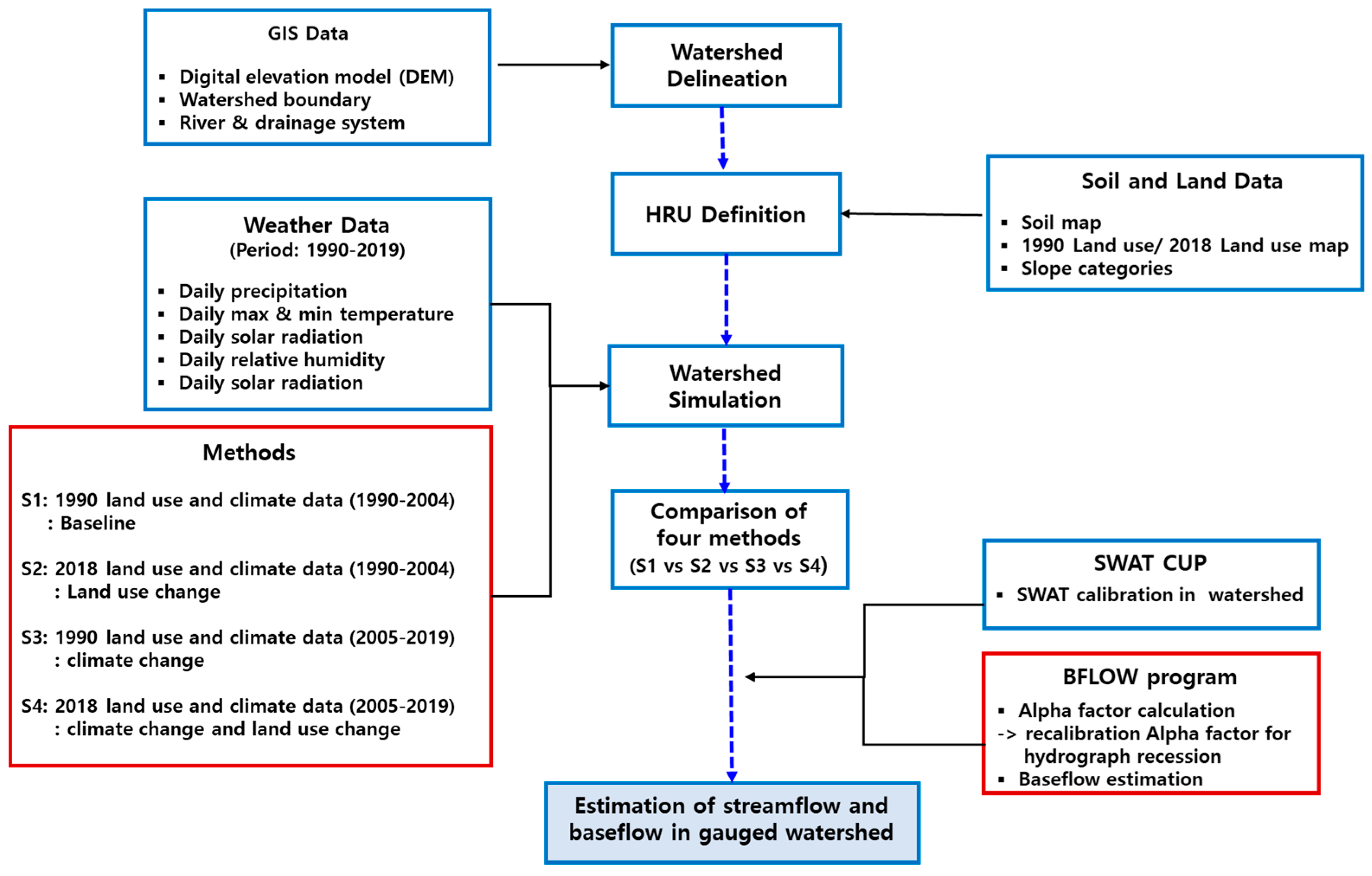
2. Methods

To evaluate the separate and combined influences of land use change and climate alteration on hydrological elements, the fix-changing approach was used, which was changed while holding others constant. Based on the change detection analysis of temporal trends of precipitation and temperature and land use change, the meteorological data from 1990–2019 were divided into two periods, with each period including one land use map. The period of 1990–2004 was called CC1 and the impacted period of 2005–2019 was called CC2. The 1990 land use map for 1990 represented the patterns in CC1, while the 2018 land use map for 2010 was used to show the patterns in CC2, assuming that minimal change existed in the watershed land use from 1990 to 2004, similarly after 2005 to 2019. Among the land use data provided by the EGIS (Environmental Geographic Information System), the oldest land use data (1990) and the most recent land use data (2018) were used for the study area. The calibrated SWAT model of Scenario 1 (or S1) was applied for each of the other three scenarios of the two meteorological periods to give four scenarios overall to evaluate the influences of land use and climate change.

For SWAT simulation, these four scenarios were developed:

• Scenario 1 (S1: Baseline): 1990 land use and CC1 climate data (1990–2004).
• Scenario 2 (S2: Land-use change): 2018 land use and CC1 climate data (1990–2004).
• Scenario 3 (S3: Climate change): 1990 land use and CC2 climate data (2005–2019).
• Scenario 4 (S4: Climate change and land use change): 2018 land use and CC2 climate data (2005–2019).

The methodology of this study involves three main steps as follows: (1) the ability of SWAT to predict runoff in a watershed is enhanced by adjusting the alpha factor related to hydrograph recession while calibration using SWAT-CUP, and (2) baseflow is estimated by applying the BFLOW program to the predicted runoff for spatiotemporally different land use and climate change. It should provide a concise and precise description of the experimental results, their interpretation, as well as the experimental conclusions that can be drawn. The procedure used in this study is shown in Figure 1.

2.1. Site Description

The Gapcheon watershed (602.22 km²) is located in the center of South Korea, as a sub-watershed of the Geum river basin (Figure 2). The watershed, in which about 1,500,000 residents live, contains Daejeon Metropolitan City, the 5th biggest city in South Korea, which has undergone extensive development during the past two decades. Daejeon city is a satellite city of the Seoul metropolitan area, and as such, has absorbed an additional 700,000 residents during the past 40 years (Figure 3). The resultant urbanization of the Gapcheon watershed has been raised as a serious issue in water resource management. SWAT calibration is performed for the Gapcheon watershed (observed), where the Wonchon monitoring station is located. The watershed is an average slope of about 28 percent. Also, the watershed has an average elevation of about 175.65 m and an average width of 10.77 km. The average annual rainfall and temperature of the watershed are about 1354 mm and 12.3 °C. Annual precipitation experienced a decrease during the past 30 years, as shown in Figure 4. The analysis showed Land use has been substantially altered from 1990 to 2018 in the Gapcheon watershed, as shown in

Table 1. Characteristics of land use change in the Gapcheon watershed from 1990 to 2018.

	Year	1990		2018		Temporal Change in Area (km2)
Land Use Type		Area (km2)	Percent (%)	Area (km2)	Percent (%)
Urbanization		42.28	7.02	75.76	12.58	33.48
Agriculture		91.30	15.16	56.07	9.31	−35.23
Forest		410.53	68.17	428.00	71.07	17.46
Pasture		29.15	4.84	24.39	4.05	−4.76
Water		2.53	0.42	2.59	0.43	0.06
Paddy		26.44	4.39	15.42	2.56	−11.02
Total		602.22	100.00	602.22	100.00	0.00

. Figure 5 indicate three land use dataset in this study. In 1990, 15.16% of the watershed land use was agriculture, 7.02% was Urbanization, 4.84% was pasture, and 4.39% was paddy. Agriculture, paddy, and pasture land use have declined, while urban areas have increased since 1990. The parts inside the dotted lines in Figure 5 represent regions where the most urbanized regions are in the study area. This means that a considerable increase is shown and urban areas (Urbanized area: +33.48 km²) in the watershed compared to other land use types (Figure 5) (Table 1). Accordingly, it is necessary to identify the hydrologic impact of land use changes and climate change in the watershed.

2.2. Data Description

The SWAT is used to assess the effects of changes in land use on streamflow and to estimate baseflow in gauged watersheds. In this regard, the simulations using SWAT are performed for two comparable periods: 1990–2004 (CC1) and 2005–2019 (CC2). Also, simulations of streamflow using SWAT require climatic data (precipitation, wind, humidity, solar radiation, and temperature) and topographic data, as well as land use and soil geographical information. Daily climatic data is available for the monitoring station of the Korea Meteorological Administration (KMA). A Digital Elevation Model (DEM) of the Gapcheon watershed is resolved with a grid size of 10 m from a numerical map at a 1:5000 scale. Also, two land use maps for the years 1990 and 2018, at a 1:25,000 scale, and a soil map were obtained from the Environmental Geographic Information System (EGIS) and the National Academy of Agricultural Science in South Korea, respectively. Streamflow data from the Wonchon monitoring station were obtained from the Water Management Information System (WAMIS) and were used to calibrate the SWAT model.

Table 2. Dataset for SWAT simulation.

Data Type	Resolution	Periods	Source
Precipitation	Temporal (1 day)	1990~2019	KMA (Korea Meteorological Administration)
Temperature	Temporal (1 day)	1990~2019	KMA (Korea Meteorological Administration)
Wind Speed	Temporal (1 day)	1990~2019	KMA (Korea Meteorological Administration)
Solar Radiation	Temporal (1 day)	1990~2019	KMA (Korea Meteorological Administration)
Humidity	Temporal (1 day)	1990~2019	KMA (Korea Meteorological Administration)
DEM (Digital Elevation Model)	Spatial	-	NGII (National Geographic Information Institute)
Land use	Spatial	1990, 2018	EGIS (Environmental Geographic Information System)
Soil	Spatial	2017	RDA (Rural Development Administration)

shows the summarized dataset used in this study.

2.3. Description of SWAT and SWAT-CUP

The SWAT is a continuous-time, long-term, and semi-distributed model for the simulation of streamflow, and water quality at the watershed scale. Many studies have been conducted to improve the accuracy of the prediction of SWAT [39,40]. Recently, Lee et al. [38] suggested that streamflow recession and baseflow were more accurately predicted when SWAT is calibrated for recession periods and baseflow with the alpha factor. For, this reason, the SWAT model has been widely applied in many countries, including the U.S., to contribute to watershed management decisions [34]. SWAT enables a watershed to be partitioned into sub-watersheds according to stream linkage which has different hydrologic data, or Hydrologic Response Units (HRU) identification, consisting of distinctive combinations of land cover, soils, and management for each sub-watershed. The computation time depends on HRU delineation, as similar soil and land use areas are considered lumped units [41]. SWAT utilizes the Penman-Monteith method, the Priestley-Taylor method, and the Hargreaves method to estimate potential evapotranspiration. Also, the NRCS curve number or the Green-Ampt infiltration method is used to estimate surface runoff based on the temporal resolution of input climatic data. In this study, the Penman-Monteith and NRCS curve numbers are used to estimate PET and runoff, respectively. The kinematic storage model, based on a mass continuity equation, is used to estimate subsurface runoff. For baseflow, SWAT simulates both a shallow aquifer which supplies return flow to streams within the watershed system, and a deep aquifer which affects streams outside the watershed [42]. In order to run SWAT, several input data are required. The observed data of this study are precipitation, daily streamflow, temperature, radiation, wind speed, topography, land use, and soil type with the datasets consisting of numerical data and maps. SWAT involves many parameters that are associated with hydrologic processes such as rainfall-runoff, and it is necessary to optimize these parameters in order to improve the accuracy of prediction. For calibration of the SWAT model, SWAT-CUP has been developed to incorporate several calibration modules for automating calibration or uncertainty analysis into SWAT. The program involves SUFI-2 [43], GLUE [44], ParaSol [45], MCMC [46], and PSO [47] in Window mode. In this study, the SUFI-2 algorithm was selected for calibration purposes and has previously been used to optimize the parameters of SWAT in several studies [43,48,49] (Figure 6).

In this study, nine parameters for calibration are efficiently selected throughout sensitivity analysis in order to determine the most significant parameters governing streamflow. Also, the performance assessment for the calibration of the SWAT model is determined by the measure of Nash Sutcliffe Efficiency (NSE), coefficient of determination (R²), index of agreement (d), PBIAS, and modified Kling-Gupta Efficiency (KGE) in this study.

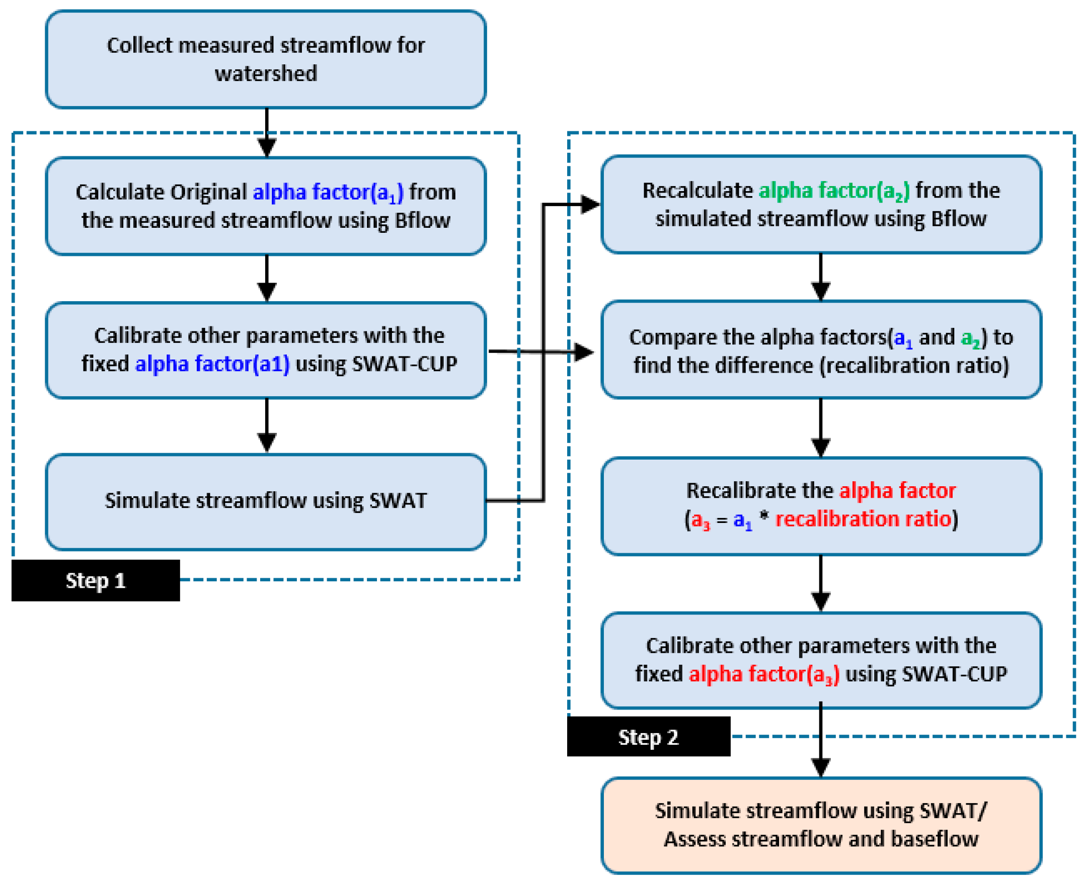
2.4. Estimation of Alpha Factor and SWAT Calibration Using the Estimated Alpha Factor

Stream recession in baseflow estimation provides important information about the natural supply of water into a stream and is strongly related to baseflow, which dominates stream water in the dry season. In this context, the stream recession affects specific parameters related to baseflow in calibrating the rainfall-runoff model. However, in SWAT calibrations conducted by numerous parameter sets, the alpha factor, which is deeply dependent on stream recession, can be distorted by various other parameters related to streamflow, including low flow. Furthermore, the alpha factor was underestimated or overestimated when analyzing the alpha factor from the simulated streamflow following calibration [50]. In such cases, it is difficult to accurately reflect the characteristics of baseflow in SWAT calibrations.

In this regard, Lee et al. [38] proposed a method in which the alpha factor is recalibrated and applied in SWAT to improve the accuracy of the recession prediction (Figure 7). Accordingly, in this study, the alpha factor is calculated by using the BFLOW program and then the alpha factor is recalibrated in order to evaluate baseflow in the Gapcheon watershed.

2.5. Baseflow Estimation Using the BFLOW Program

The digital filter can provide multiple passes through the filter (first pass, second pass, and third pass) (Equations (1) and (2)), allowing users to select and use the desired number of passes to calculate the baseflow for the streamflow [29].

$$F_t= \mathsf{\alpha } * F_{t-1}+\frac{1+\mathsf{\alpha }}{2} * \left(Q_t-Q_{t-1}\right)$$

(1)

$$B_t=Q_t-F_t, 0\le B_t\le Q_t$$

(2)

where $B_t$ is the baseflow, $\mathsf{\alpha }$ is the filter parameter (0.925), $Q_t$ is the total streamflow, $F_t$ is the filtered surface runoff (quick response) and t is the time step (one day). The value of 0.925 was determined by Nathan and McMahon [26] and Arnold et al. [51] to give realistic results when compared to manual separation techniques.

It is commonly observed that the first pass baseflow is consistent with manually calculated baseflow. Moreover, Ahiablame et al. [52] constructed a regression equation to estimate baseflow within the state of Indiana for ungagged watersheds and calculated the baseflow that was used to create the equation using measured data from the first pass of the BFLOW program. In this study, the first pass results were used. The baseflow was separated from the streamflow provided by the Wonchon monitoring station. Accordingly, the effect of land use change and climate on baseflow is quantified by applying the BFLOW program to streamflow estimations from SWAT simulations.

2.6. Evaluation of Streamflow and Baseflow Estimation from Scenarios

In this study, the streamflow of the Gapcheon watershed was predicted using weather data from the period 1990 to 2019. Following Moriasi et al. [53], graphical comparison and statistical indices can assess the performance of the calibrated parameters. The conformance assessment for the calibration of the SWAT model is determined by the coefficient of determination (R²), Nash Sutcliffe Efficiency (NSE), Kling-Gupta Efficiency (KGE), Root Mean Squared Errors (RMSE), and the Mean Absolute Error (MAE) for the simulated streamflow and baseflow (Equations (3)–(9)). An NSE, R, and R² value of “1” indicates perfect agreement between observations and simulations. The modified index of the agreement also varies from 0 to 1 with higher values indicating a better fit of the model.

Singh et al. [54] state that MAE and RMSE values less than half the standard deviation of the measured data may be considered low, and either is appropriate for model evaluation. RMSE is the standard deviation of the residuals, and MAE is the mean of the absolute values of the errors. Therefore, meaning that the closer the verification values are to zero, the more similar the observed and the model values are.

$$\mathrm{NSE}=1-\frac{{{\displaystyle \sum }}_{\mathrm{i}=1}^{\mathrm{n}}{({\mathrm{Y}}_{\mathrm{i}}^{\mathrm{obs}}-{\mathrm{Y}}_{\mathrm{i}}^{\mathrm{sim}})}^2}{{{\displaystyle \sum }}_{\mathrm{i}=1}^{\mathrm{n}}{({\mathrm{Y}}_{\mathrm{i}}^{\mathrm{obs}}-{\overline{\mathrm{Y}}}^{\mathrm{obs}})}^2}$$

(3)

$${\mathrm{R}}^2=\frac{{({{\displaystyle \sum }}_{\mathrm{i}=1}^{\mathrm{n}}\left({\mathrm{Y}}_{\mathrm{i}}^{\mathrm{obs}}-{\overline{\mathrm{Y}}}^{\mathrm{obs}}\right)\left({\mathrm{Y}}_{\mathrm{i}}^{\mathrm{sim}}-{\overline{\mathrm{Y}}}^{\mathrm{sim}}\right))}^2}{({{\displaystyle \sum }}_{\mathrm{i}=1}^{\mathrm{n}}{({\mathrm{Y}}_{\mathrm{i}}^{\mathrm{obs}}-{\overline{\mathrm{Y}}}^{\mathrm{obs}})}^2{{\displaystyle \sum }}_{\mathrm{i}=1}^{\mathrm{n}}{({\mathrm{Y}}_{\mathrm{i}}^{\mathrm{sim}}-{\overline{\mathrm{Y}}}^{\mathrm{sim}})}^2}$$

(4)

$$\mathrm{KGE}=1-\sqrt{{\left(\mathsf{\gamma }-1{)}^2+{(\mathsf{\beta }-1)}^2(\mathrm{r}-1\right)}^2}$$

(5)

where

$$\mathsf{\gamma }=\frac{C{V}^{sim}}{C{V}^{obs}}=\frac{\frac{{\sigma }^{sim}}{{\mu }^{sim}}}{\frac{{\sigma }^{obs}}{{\mu }^{obs}}}$$

(6)

and

$$\mathsf{\beta }=\frac{{\mu }^{sim}}{{\mu }^{obs}}$$

(7)

$$RMSE=\sqrt{\frac{{{\displaystyle \sum }}_{i=1}^n{(Y_i^{obs}-Y_i^{sim})}^2}{n}}$$

(8)

$$MAE = \frac{1}{n}\sum |Y_i^{sim}-Y_i^{obs}|$$

(9)

where $Y_i^{obs}$ is the observed data, ${\overline{Y}}^{obs}$ is the mean of the actual value, $Y_i^{sim}$ is the estimated value of t, ${\overline{Y}}^{obs}$ is the mean of the estimated value, and n is the total number of times.

The $\mathsf{\gamma }$ is the variation coefficient ratio between the simulated ($C{V}^{sim})$ and the observed $(C{V}^{obs})$ flow, in which ${\sigma }^{sim}$ and ${\sigma }^{obs}$ represent the standard deviations of both measured and simulated data, respectively; $\mathsf{\beta }$ is the ratio between the simulated mean (${\mu }^{sim})$ and the observed mean $\left({\mu }^{obs}\right)$ flow, $r$ is the correlation between the measured and simulated values.

3. Results and Discussion

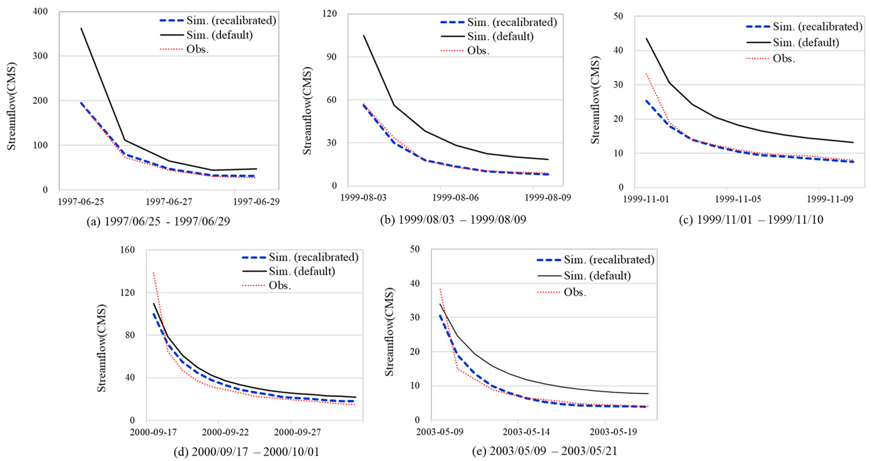
3.1. Calibration and Validation Results of SWAT Consider to Recession Curve

It is necessary to accurately predict streamflow in gauged watersheds in order to estimate baseflow according to the effect of land use and climate change. This study calibrates the SWAT model for streamflow observed from a monitoring station (Wonchon) in the Gapcheon watershed and attempts to improve streamflow predictions using SWAT. The sensitivity analysis (

Table 3. List of twelve sensitive parameters for SWAT in the study area.

Rank	Parameter Name	p-Value	t-Stat
1	CH_K2	0	−23.36
2	ALPHA_BF	0	12.29
3	SLSUBBSN	0	−2.80
4	SURLAG	0.02	2.35
5	CN2	0.11	1.62
6	SOL_K	0.11	1.60
7	HRU_SLP	0.20	−1.29
8	CANMX	0.20	−1.28
9	ESCO	0.30	−1.04
10	SOL_AWC	0.34	−0.95
11	EPCO	0.45	0.76
12	GWQMN	0.82	0.22

) shows that, in general, CH_K2, ALPHA_BF, SLSUBBSN, SURLAG, CN2, and SOL_K are the sensitive and essential parameters for the watershed, as they show larger absolute values of t-statistics and their p-values are significant. The sensitivity parameters analysis showed that parameters representing surface runoff, soil properties, and groundwater return flow are sensitive [55]. The most sensitive parameter is the effective hydraulic conductivity of the main channel (CH_K2), followed by the baseflow recession alpha factor (Alpha_BF) which could affect the shape of the streamflow hydrograph, and is identified as a parameter with a second sensitivity rank. The quick recession and steep nature of the streamflow could partly explain this hydrograph due to the mountainous area, which are the specific characteristics of the Gapcheon watersheds [56]. The estimation of the alpha factor was 0.0175 using the BFLOW program to consider the physical characteristics of recession in order to improve the accuracy in the SWAT. In this study, the alpha factor was recalibrated using the method proposed by Lee et al. [38] in order to properly reflect the calculated alpha factor from measured streamflow data (Figure 7). The recalibrated alpha factor value was 0.045 and then this value was used as a fixed parameter in SWAT-CUP.

This indicates that the alpha factor value obtained from baseflow filtering is low and appears to be inappropriate for SWAT, providing poor calibration. The discrepancy between the value derived by the baseflow filter program and SWAT may be due to the empirical nature of the method and its lack of realistic representation of the watershed characteristics [57]. As mentioned earlier, the recalibrated alpha factor value in the stream part of the watershed likely reflects this effect-related recession curve.

The results of calibration and validation are shown in

Table 4. Values of statistical indicators in the calibration and validation periods for streamflow and baseflow.

Period	Streamflow (m3/s)					Baseflow (m3/s)
	NSE	R2	KGE	RMSE	MAE	NSE	R2	KGE	RMSE	MAE
Calibration (1994–2004)	0.66	0.71	0.52	9.98	9.97	0.59	0.64	0.70	8.03	5.16
Validation (2005–2008)	0.70	0.75	0.63	6.60	6.61	0.73	0.75	0.78	5.85	3.29

. The calibration results from the S1 method show an NSE of 0.66, R² of 0.71, KGE of 0.52, RMSE of 9.98, and MAE of 9.97. Moreover, the validation achieved was an NSE of 0.70, R² of 0.75, KGE of 0.63, RMSE of 6.60, and MAE of 6.61. The performance of the SWAT for streamflow simulation was considered “Satisfactory” in the evaluation criteria of calibration and validation based on the guidance in Moriasi et al. [53].

Figure 7 and Figure 8 show the simulated (default: step1, recalibrate: step2) streamflow and observed streamflow recession (extracted) as an example of a comparison of the recession curves. It indicates that the recession simulations were a similar trend which means that the simulated streamflow showed a reasonable match with the observed records. Furthermore, the accuracy of streamflow and baseflow was improved due to the recalibrated alpha factor. These statistical outputs indicated that the simulated baseflow in calibration and validation was in “Good” agreement, according to Singh et al. [54] criteria. Table 4 shows that compared to the streamflow results, the highest values of KGE, R², RMSE, and MAE were found for the watershed for the baseflow results.

This is because the alpha factor was applied to the SWAT-CUP calibration after multiplying the calculated alpha factor from the measured streamflow data by approximately 2.57 (recalibration ratio) proposed (Figure 7). This means that baseflow prediction in SWAT could be improved by taking into account the recession characteristics correctly. The alpha factor should have to consider measured streamflow data. This means that the alpha factor can be applied differently according to the characteristics of the watershed such as the weather data. Lee et al. [38] reported when applying the alpha factor in the SWAT model to five study areas with different watershed characteristics (land use, slope, etc.) in South Korea, it is suggested to apply the alpha factor at a recalibration ratio of approximately two or a little more (difference or recalibration ratio). In addition, by applying the recalibrated alpha factor in the SWAT, the prediction results of streamflow and baseflow were more accuracy improved. Subsequently, although the five study area characteristics are different compared to those in this study (Gapcheon watershed), it is essential to the consider recession curve in order to improve the prediction of streamflow and baseflow.

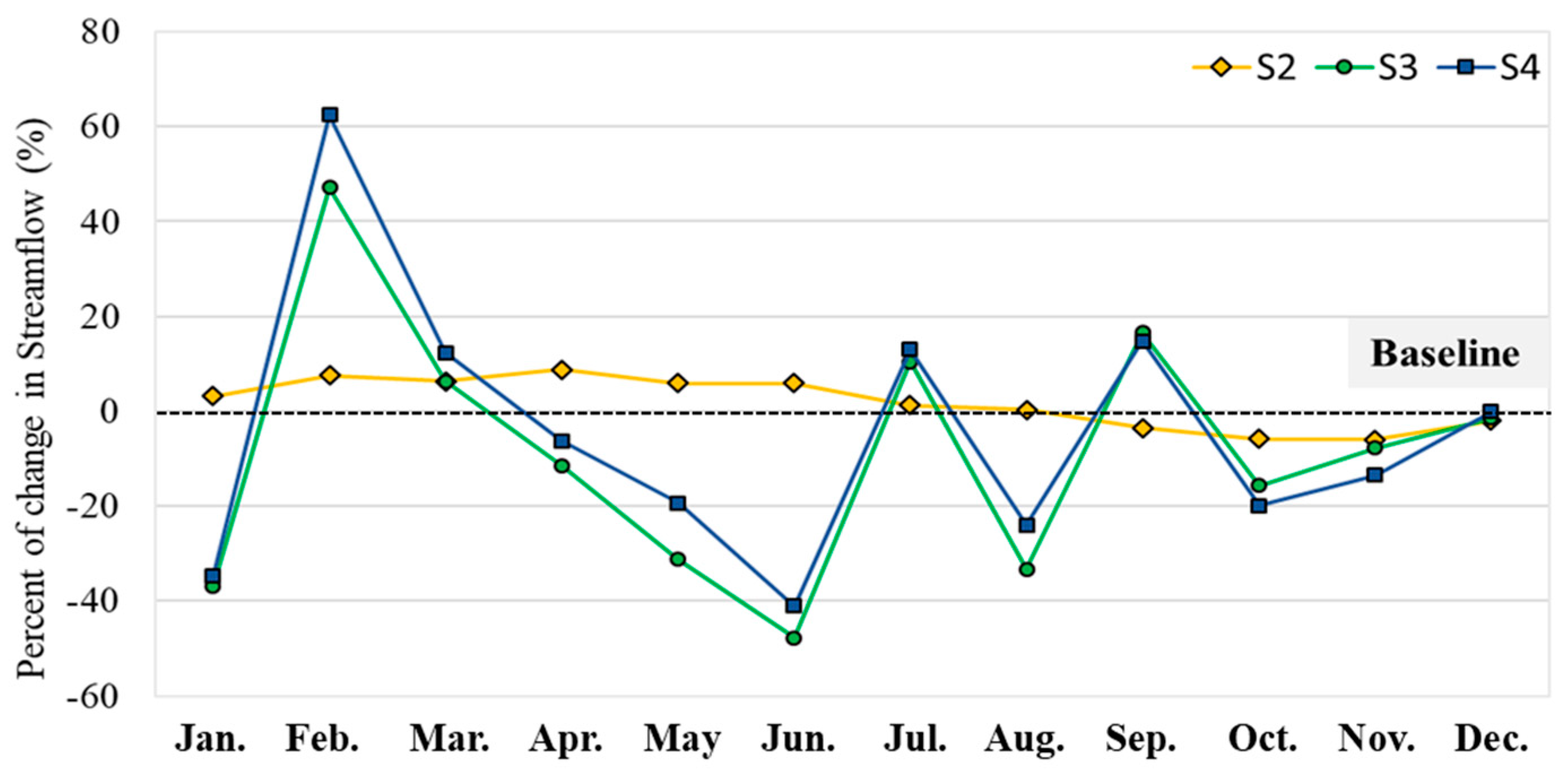
3.2. Change in Streamflow and Baseflow according to Land Use Climate Change Scenarios

Table 5. Comparison of average annual change in study watershed.

No.	Climate	Average Precipitation (mm)	Land Use	Streamflow (mm)			Surface Runoff (mm)			Baseflow (mm)
				Average	Percent (%)	Change	Average	Percent (%)	Change	Average	Percent (%)	Change
S1	CC1	1398.2 (Max: 2070.0) (Min: 828.7)	1990	705.6	-	-	578.8	-	-	126.8	-	-
S2	CC1	1398.2 (Max: 2070.0) (Min: 828.7)	2018	725.5	2.8%	19.9	620.8	7.3%	42.0	104.7	−17.4%	−22.1
S3	CC2	1296.5 (Max: 1943.4) (Min: 822.6)	1990	629.8	−10.7%	−75.8	515.2	−11.0%	−63.6	114.6	−9.6%	−12.2
S4	CC2	1296.5 (Max: 1943.4) (Min: 822.6)	2018	649.4	−8.0%	−56.2	555.8	−4.0%	−23.0	93.6	−26.2%	−33.2

explains the simulated SWAT annual average streamflow and baseflow under different scenarios of climate and land use change in the study watershed. Results illustrated that the difference in average annual streamflow between S2 and S1, which simulated the impacts of land use change, showed an increase of 19.9 mm (2.8%). Compared to S1, the average annual streamflow decreased by −75.8 mm (−10.7%), which demonstrated the impacts of climate variation. Meanwhile, the average annual streamflow decreased by −56.2 mm (−8.0%) due to the combined effects of climate variation and land use change. These findings show that indicate that the average annual streamflow decreased during CC1 and CC2 due to climate change, such as precipitation. It is the influence of climate change greater than land use dynamics. Therefore, the contribution of the combined impacts was higher than land use change and climate change separately.

However, the simulation suggested an increase in the average annual surface runoff (mm) due to the effect of land use change, even though decreasing baseflow between S1 and S2. In other words, urban expansion had a significant impact on annual streamflow by increasing the impervious area and decreasing infiltration. Table 5 shows that the average annual baseflow decreased by −22.1 mm (−17.4%), which demonstrated the impacts of land use dynamics compared to S1. The contribution of climate change and land use change separately impacts were lower than combined impacts. Climate variation has increased the negative impact of land use change by 21.0 mm as it increased from S4 (−26.2%) to S3 (−9.63%).

The baseflow index (BFI) was analyzed based on simulated streamflow using BFLOW. The BFI represents the characteristics of aquifers in the watershed and plays an important role in determining the characteristics of the runoff. The BFI results of scenario (1~4) were calculated dry season (S1; 31.2%, S2; 27.3%, S3: 33.0%, S4; 29.8%) and wet season (S1; 18.4%, S2; 16.0%; S3; 17.7%, S4; 14.1%). The dry season was divided into January to May and October to December, and the wet season from June to September. Among the four scenarios in dry seasons, S3, in which the baseflow rate is highest when compared to the surface runoff, has the largest value of BFI, while S2 has the smallest value of BFI. The land use in S2 is impervious increase due to urbanization relative to another Scenario 3. Through these results, it is necessary to maintain and manage baseflow in the dry season than in the wet season. Although baseflow increased due to precipitation variation in climate change, according to the results of scenario 4, the baseflow ratio decreased due to land use and other factors.

The distribution of precipitation and temperature was divided into 10-year units and analyzed (average, maximum, minimum, and median), as shown in

Table 6. Trend analysis of average annual precipitation and temperature pattern.

Year	Average Annual Precipitation				Average Annual Temperature
	Average (mm)	Maximum (mm)	Minimum (mm)	Median (mm)	Maximum (°C)	Minimum (°C)
Year 1 (1990–2000)	1381.3	2070.0	857.39	1455.2	34.8	−13.5
Year 2 (2001–2010)	1360.3	1750.9	828.7	1399.2	33.8	−13.6
Year 3 (2011–2019)	1255.2	1943.4	822.6	1127.5	36.4	−13.8

. As a result of the analysis, in recent years, except for the average annual maximum precipitation of 1943.4 mm, precipitation changes tended to decrease (mean, minimum, median). Moreover, the temperature trend also increased by approximately 2 °C in Year 3 (2011–2019) compared to Year 1 (1990–2000). It is analyzed that this precipitation decrease pattern and temperature increase trend have a significant effect on the decrease of not only streamflow but also baseflow.

Figure 9 shows the average monthly streamflow changes relative to the baseline scenario (S1). Compared to S1, annual runoff exhibited small changes, monthly runoff the medium changes (increasing in all months except September to November) in S2, because of variable influence on evapotranspiration and antecedent soil water storage. In the case of S2, same climate conditions, land use is changed. The land use changed by decreasing agriculture and paddy areas and increasing urbanized areas from 1990 to 2018.

Figure 10 shows the temporal distributions in monthly baseflow changes relative to the baseline scenario (S1). Compared to scenario 1, the percent of change in streamflow increased from February to March, and the percent of change in baseflow increased from March to April in scenarios 3 and 4. Baseflow decreases due to the increase in the impermeable area of urban areas, despite heavy rains in summer. For comparing S1–S2 and S3–S4, Baseflow decreased by an average of 27.63%, this is because the location of the urbanized area is near the outlet of the watershed which derived an immediate increase in the streamflow. Despite heavy rains in the summer, the baseflow decreases due to the increase in the impermeable area in urban areas. The monthly baseflow at the Gapcheon watershed was the largest in April (dry season) and the smallest in June (wet season). This is possible because the surface runoff in the marginal region flows into the central region with a mild slope due to the high precipitation.

Our findings in this study are similar to the results of land use change [58,59,60]. Siddik et al. [58] found that urbanization-dominated land use change has been observed to have a significant influence on baseflow. The land use change in recent decades is significantly higher than in previous decades. Mojid and Mainuddin [59] reported that increased urbanization might have an effect on declining baseflow. Kim et al. [60] indicated that in the case of considering only the land use change scenario, as the urban area with many impervious increases and the permeable space decreases, total streamflow and surface runoff increase while the baseflow decreases.

4. Conclusions

It is of vital significance to understand the behaviors of hydrologic components under the separate and combined impacts of climate variation and land use dynamics. This means that rainfall variation and urbanization play a significant role in altering the Spatiotemporal distribution of water resources. In particular, streamflow and baseflow are crucially important hydrology components that are essential to sustain water demands by various sectors. In this study, the SWAT was used to calibrate and validate streamflow and baseflow from 1990 to 2019 to determine the separate impact of climate variability and urbanization at the Gapcheon watershed. Moreover, the automated SUFI-2 approach and baseflow recession method helped in minimizing the discrepancies between the observed and simulated data. The following conclusions were drawn in this study.

(1)

In this study, Lee et al. [38] as the method proposed, the predictability of the base flow and low flow intervals is improved by considering the characteristics of the reducing section. Through these results, the variability of runoff and base runoff due to land use and climate change was analyzed. When analyzing using the SWAT model in various studies in the future, it is judged to be more effective only when flow rate and base flow rate analysis are performed after considering the characteristics of the reducing part.

(2)

In the case of Scenario 2, the impervious urban area increased, and the agricultural area, the permeability area, decreased. Compared to the baseline (Scenario 1), the total streamflow increased while the baseflow decreased. According to the hydrologic variation research results, land-use change with an increase in significant urbanization and a gradual decrease in agriculture and paddy area. Scenario 4, which analyzed both climate change and land-use change, showed similar trends in streamflow fluctuation to Scenario 3, which considered only climate change.

(3)

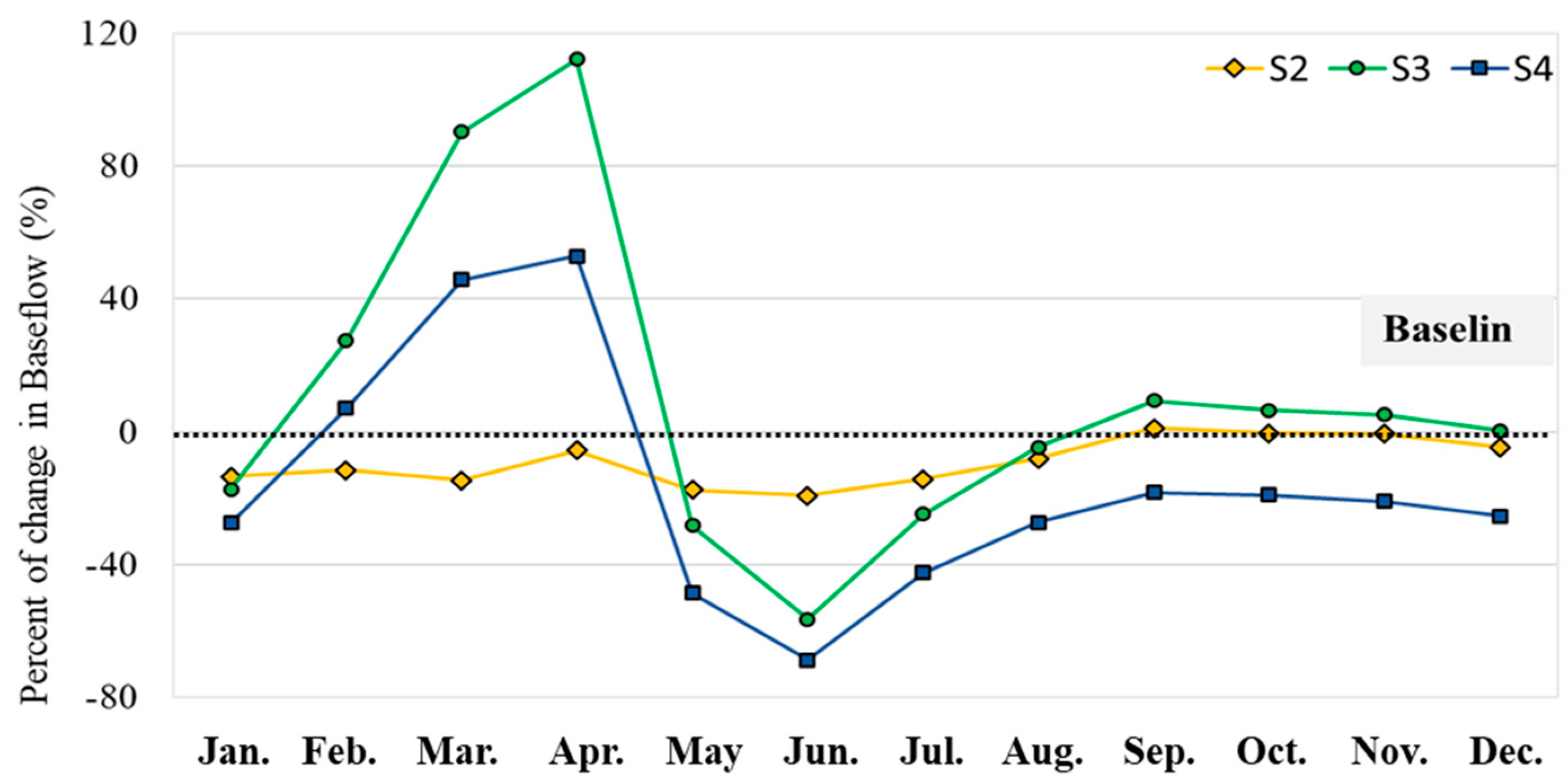
According to the results of the monthly streamflow and baseflow analysis, in Scenario 2, streamflow increased due to increased precipitation in summer, and baseflow decreased due to an increase in impervious area. Also, the amount of streamflow showed a tendency to decrease in the fall/winter season. Compared to the baseline in Scenario 1, Scenarios 3–4 showed large flow fluctuations in February and March, and then the baseflow was delayed with large fluctuations in March and April. The baseflow lag time is due to the study area’s steep slope topographical factors and soil properties.

(4)

It finds study area is vulnerable to both changes due to rapid population growth, precipitation changes due to climate change, land covers, and land-use change. Based on this study, findings will provide practical suggestions for environmental researchers and hydrology researchers on how to retain water resources more efficiently concerning its variability as a response to climate change and land use. The outcomes of this study can be used in quantifying the potential impacts of future projected climate change and land use change. Therefore, more studies need to evaluate this potential future impact on the hydrological system, with an emphasis on the interactive effect of environmental change drivers when predicting future change.

References

- Ferguson, G.; Gleeson, T. Vulnerability of coastal aquifers to groundwater use and climate change. Nat. Clim. Chang. 2012, 2, 342–345. [Google Scholar] [CrossRef]
- Lee, J.; Lee, S.; Hong, J.; Lee, D.; Bae, J.H.; Yang, J.E.; Kim, J.; Lim, K.J. Evaluation of rainfall erosivity factor estimation using machine and deep learning models. Water 2021, 13, 382. [Google Scholar] [CrossRef]
- Li, R.; Merchant, J.W. Modeling vulnerability of groundwater to pollution under future scenarios of climate change and biofuels-related land use change: A case study in North Dakota, USA. J. Sci. Total Environ. 2013, 447, 32–45. [Google Scholar] [CrossRef]
- Lee, J.; Kim, J.; Lee, J.M.; Jang, H.S.; Park, M.; Min, J.H.; Na, E.H. Analyzing the Impacts of Sewer Type and Spatial Distribution of LID Facilities on Urban Runoff and Non-Point Source Pollution Using the Storm Water Management Model (SWMM). Water 2022, 14, 2776. [Google Scholar] [CrossRef]
- Haddelanda, I.; Heinkeb, J.; Biemansd, H.; Eisnere, S.; Florkee, M.; Hanasakif, N.; Konzmannb, M.; Ludwigd, F.; Masakif, Y.; Scheweb, J.; et al. Global water resources affected by human interventions and climate change. Proc. Natl. Acad. Sci. USA 2014, 111, 3251–3256. [Google Scholar] [CrossRef]
- George, Z.N.; Woyessa, Y. Evaluation of streamflow under climate change in the Zambezi River basin of Southern Africa. Water 2021, 13, 3114–3134. [Google Scholar]
- Lee, J.; Ryu, J.C.; Kang, H.W.; Kum, D.H.; Jang, C.H.; Choi, J.D.; Lim, K.J. Evaluation of SWAT flow and sediment estimation and effects of soil erosion best management practices. J. Korean Soc. Agric. Eng. 2012, 54, 99–108. [Google Scholar] [CrossRef]
- Lee, J.; Shin, Y.; Park, Y.S.; Kum, D.; Lim, K.J.; Lee, S.O.; Kim, H.; Jung, Y. Estimation and assessment of baseflow at an ungauged watershed according to landuse change. J. Wetl. Res. 2014, 16, 303–318. [Google Scholar]
- Shuster, W.D.; Bonta, J.; Thurston, H.; Warnemuende, E.; Smith, D.R. Impacts of impervious surface on watershed hydrology: A review. J. Urban Water 2005, 2, 263–275. [Google Scholar] [CrossRef]
- Ogden, F.L.; Raj, P.N.; Downer, C.W.; Zahner, J.A. Relative importance of impervious area, drainage density, width function, and subsurface storm drainage on flood runoff from an urbanized catchment. J. Water Resour. Res. 2011, 47, 1–12. [Google Scholar] [CrossRef]
- Kim, S.J.; Kwon, H.J.; Park, G.; Lee, M.S. Assessment of land-use impact on streamflow via a grid-based modelling approach including paddy fields. J. Hydrol. Process. 2005, 19, 3801–3817. [Google Scholar] [CrossRef]
- Gao, Y.Z.; Giese, M.; Han, X.G.; Wang, D.L.; Zhou, Z.Y.; Brueck, H.; Lin, S.; Taube, F. Land use and drought interactively affect interspecific competition and species diversity at the local scale in a semiarid steppe ecosystem. J. Ecol. Res. 2009, 24, 627–635. [Google Scholar] [CrossRef]
- Maneta, M.P.; Torres, M.D.O.; Wallender, W.W.; Vosti, S.; Howitt, R.; Rodrigues, L.; Bassoi, L.H.; Panday, S. A spatially distributed hydro economic model to assess the effects of drought on land use, farm profits, and agricultural employment. J. Water Resour. Res. 2009, 45, W11412. [Google Scholar] [CrossRef]
- De Moel, H.; Aerts, J.C.J.H. Effect of uncertainty in land use, damage models and inundation depth on flood damage estimates. J. Nat. Hazards 2011, 58, 407–425. [Google Scholar] [CrossRef]
- Wheater, H.S.; Ballard, C.; Bulygina, N.; McIntyre, N.; Jackson, B.M. Modelling Environmental Change: Quantification of Impacts of Land Use and Land Management Change on UK Flood Risk. J. Syst. Identif. Environ. Model. Control Syst. Des. 2012, 22, 449–481. [Google Scholar]
- Hamel, P.; Daly, E.; Fletcher, T.D. Source-control stormwater management for mitigating the impacts of urbanization on baseflow: A review. J. Hydrol. 2013, 485, 201–211. [Google Scholar] [CrossRef]
- Malhi, Y.; Aragão, L.E.; Galbraith, D.; Huntingford, C.; Fisher, R.; Zelazowski, P.; Sitch, S.; Mc Sweeney, C.; Meir, P. Exploring the likelihood and mechanism of a climate-change-induced dieback of the Amazon rainforest. Proc. Natl. Acad. Sci. USA 2009, 106, 20610–20615. [Google Scholar] [CrossRef] [PubMed]
- Wang, L.; Lyons, J.; Kanehl, P.; Bannerman, R. Impacts of urbanization on stream habitat and fish across multiple spatial scales. J. Environ. Manag. 2001, 28, 255–266. [Google Scholar] [CrossRef]
- Price, K. Effects of watershed topography, soils, land use, and climate on baseflow hydrology in humid regions: A review. J. Geogr. Phys. 2011, 35, 465–492. [Google Scholar] [CrossRef]
- Hall, F.R. Base-Flow Recessions-A Review. J. Water Resour. Res. 1968, 4, 973–983. [Google Scholar] [CrossRef]
- Sophocleous, M. Interactions between groundwater and surface water: The state of the science. J. Hydrogeol. 2002, 10, 52–67. [Google Scholar] [CrossRef]
- Santhi, C.; Allen, P.M.; Muttiah, R.S.; Arnold, J.G.; Tuppad, P. Regional estimation of base flow for the conterminous United States by hydrologic landscape regions. J. Hydrol. 2008, 351, 139–153. [Google Scholar] [CrossRef]
- Ward, R.C.; Robinson, M. McGraw-Hill International UK Limited, UK. J. Princ. Hydrol. 1990, 365. [Google Scholar]
- Lee, J.; Park, Y.S.; Jung, Y.; Cho, J.; Yang, J.E.; Lee, G.; Kim, K.S.; Lim, K.J. Analysis of spatiotemporal changes in groundwater recharge and baseflow using SWAT and BFlow Models. J. Korean Soc. Water Environ. 2014, 30, 549–558. [Google Scholar] [CrossRef]
- Avesani, D.; Galletti, A.; Piccolroaz, S.; Bellin, A.; Majone, B. A dual-layer MPI continuous large-scale hydrological model including Human Systems. Environ. Model. Softw. 2021, 139, 105003. [Google Scholar] [CrossRef]
- Nathan, R.J.; McMahon, T.A. Evaluation of automated techniques for base flow and recession analyses. J. Water Resour. Res. 1990, 26, 1465–1473. [Google Scholar] [CrossRef]
- Tallaksen, L.M. A review of baseflow recession analysis. J. Hydrol. 1995, 165, 349–370. [Google Scholar] [CrossRef]
- Szilagyi, J.; Parlange, M.B. Baseflow separation based on analytical solutions of the Boussinesq equation. J. Hydrol. 1998, 204, 251–260. [Google Scholar] [CrossRef]
- Arnold, J.G.; Allen, P.M. Validation of Automated Methods for Estimating Baseflow and Groundwater Recharge from Stream Flow Records. J. Am. Water Resour. Assoc. 1999, 35, 411–424. [Google Scholar] [CrossRef]
- Ahiablame, L.; Chaubey, I.; Engel, B.; Cherkauer, K.; Merwade, V. Estimation of annual baseflow at ungauged sites in Indiana USA. J. Hydrol. 2013, 476, 13–27. [Google Scholar] [CrossRef]
- Bako, M.D.; Owoade, A. Field application of a numerical method for the derivation of baseflow recession constant. J. Hydrol. Process. 1988, 2, 331–336. [Google Scholar] [CrossRef]
- Wilcox, B.P.; Huang, Y. Woody plant encroachment paradox: Rivers rebound as degraded grasslands convert to woodlands. J. Geophys. Res. Lett. 2010, 37. [Google Scholar] [CrossRef]
- Samuel, J.; Coulibaly, P.; Metcalfe, R.A. Identification of rainfall–runoff model for improved baseflow estimation in ungauged basins. J. Hydrol. Process. 2012, 26, 356–366. [Google Scholar] [CrossRef]
- Gitau, M.W.; Chaubey, I. Regionalization of SWAT model parameters for use in ungauged watersheds. J. Water 2010, 2, 849–871. [Google Scholar] [CrossRef]
- Singh, A.; Imtiyaz, M.; Isaac, R.K.; Denis, D.M. Comparison of soil and water assessment tool (SWAT) and multilayer perceptron (MLP) artificial neural network for predicting sediment yield in the Nagwa agricultural watershed in Jharkhand, India. J. Agric. Water Manag. 2012, 104, 113–120. [Google Scholar] [CrossRef]
- Eckhardt, K. How to construct recursive digital filters for baseflow separation. J. Hydrol. Process. 2005, 19, 507–515. [Google Scholar] [CrossRef]
- Eckhardt, K. A comparison of baseflow indices, which were calculated with seven different baseflow separation methods. J. Hydrol. 2008, 352, 168–173. [Google Scholar] [CrossRef]
- Lee, J.; Kim, J.; Jang, W.S.; Lim, K.J.; Engel, B. Assessment of Baseflow estimates considering recession characteristics in SWAT. Water 2018, 10, 371–385. [Google Scholar] [CrossRef]
- Chaplot, V. Impact of DEM mesh size and soil map scale on SWAT runoff, sediment, and NO3–N loads predictions. J. Hydrol. 2005, 312, 207–222. [Google Scholar] [CrossRef]
- Jeong, J.; Kannan, N.; Arnold, J.; Glick, R.; Gosselink, L.; Srinivasan, R.; Harmel, D. Development of Sub Daily Erosion and Sediment Transport Models in SWAT. Trans. ASABE 2011, 54, 1685–1691. [Google Scholar] [CrossRef]
- Neitsch, S.L.; Arnold, J.G.; Kiniry, J.R.; Williams, J.R.; King, K.W. Soil and Water Assessment Tool: Theoretical Documentation, Version 2005; Texas Water Resources Institute: College Station, TX, USA, 2005. [Google Scholar]
- Arnold, J.G.; Allen, P.M.; Bernhardt, G. A comprehensive surface-groundwater flow model. J. Hydrol. 1993, 142, 47–69. [Google Scholar] [CrossRef]
- Abbaspour, K.C.; Yang, J.; Maximov, I.; Siber, R.; Bonger, K.; Mieleitner, J.; Zobrist, J.; Srinivasan, R. Modelling Hydrology and Water Quality in the Pre-alpine Thur Watershed using SWAT. J. Hydrol. 2007, 333, 413–430. [Google Scholar] [CrossRef]
- Beven, K.J.; Binley, A.M. The future of distributed models: Model calibration and uncertainty prediction. J. Hydrol. Process. 1992, 6, 279–298. [Google Scholar] [CrossRef]
- Van Griensven, A.; Meixner, T. Methods to quantify and identify the sources of uncertainty for river basin water quality models. J. Water Sci. Technol. 2006, 53, 51–59. [Google Scholar] [CrossRef] [PubMed]
- Kuczera, G.; Parent, E. Monte Carlo assessment of parameter uncertainty in conceptual catchment models: The Metropolis algorithm. J. Hydrol. 1998, 211, 69–85. [Google Scholar] [CrossRef]
- Eberhart, R.; Kennedy, J. A new optimizer using particle swarm theory. In Proceedings of the Sixth International Symposium on Micro Machine and Human Science, MHS’95, Nagoya, Japan, 4–6 October 1995; pp. 39–43. [Google Scholar]
- Rostamian, R.; Jaleh, A.; Afyuni, M.; Mousavi, S.F.; Heidarpour, M.; Jalalian, A.; Abbaspour, K.C. Application of a SWAT model for estimating runoff and sediment in two mountainous basins in central Iran. J. Hydrol. Sci. 2008, 53, 977–988. [Google Scholar] [CrossRef]
- Abbaspour, K.C. SWAT-CUP4: SWAT Calibration and Uncertainty Programs—A User Manual; EAWAG Swiss Federal Institute of Aquatic Science and Technology: Dubendorf, Switzerland, 2011; pp. 1–103. [Google Scholar]
- Leta, O.T.; El-kadi, A.I.; Dulai, H.; Ghazal, K.A. Assessment of climate change impacts on water balance components of Heeia watershed in Hawaii. J. Hydrol. Reg. Stud. 2016, 8, 182–197. [Google Scholar] [CrossRef]
- Arnold, J.G.; Allen, P.M.; Muttiah, R.; Bernhardt, G. Automated baseflow separation and recession analysis techniques. Groundwater 1995, 33, 1010–1018. [Google Scholar] [CrossRef]
- Ahiablame, L.; Engel, B.; Chaubey, I. Representation and evaluation of low impact development practices with L-THIA-LID: An example for planning. Environ. Pollut. 2012, 1, 1. [Google Scholar] [CrossRef]
- Moriasi, D.N.; Arnold, J.G.; Van Liew, M.W.; Bingner, R.L.; Harmel, R.D.; Veith, T.L. Model evaluation buidelines for systematic quantification of accuracy in watershed simulations. Am. Soc. Agric. Biol. Eng. 2007, 50, 885–900. [Google Scholar]
- Singh, J.; Knapp, H.V.; Arnold, J.G.; Demissie, M. Hydrologic modeling of the Iroquois river watershed using HSPF and SWAT. J. Am. Water Resour. Assoc. 2005, 41, 361–375. [Google Scholar] [CrossRef]
- Jang, W.S.; Engel, B.; Ryu, J. Efficient flow calibration method for accurate estimation of baseflow using a watershed scale hydrological model (SWAT). Ecol. Eng. 2018, 125, 50–67. [Google Scholar] [CrossRef]
- Izuka, S.K.; Hill, B.R.; Shade, P.J.; Tribble, G.W. Geohydrology and Possible Transport Routes of Polychlorinated Biphenyls in Haiku Valley, Oahu Hawaii; Water-Resources Investigations Report; USGS: Reston, VA, USA, 1993. [Google Scholar]
- Furey, P.R.; Gupta, V.K. A physically based filter for separating base flow from streamflow time series. Water Resour. Res. 2001, 37, 2709–2722. [Google Scholar] [CrossRef]
- Siddik, S.; Tulip, S.S.; Rahman, A.; Islam, N.; Haghighi, A.T.; Mustafa, S.M.T. The impact of land use and land cover change on groundwater recharge in northwestern Bangladesh. J. Environ. Manag. 2022, 315, 115130. [Google Scholar] [CrossRef] [PubMed]
- Mojid, M.A.; Mainuddin, M. Water-saving agricultural technologies: Regional hydrology outcomes and knowledge gaps in the eastern gangetic plains—A review. Water 2021, 13, 636. [Google Scholar] [CrossRef]
- Kim, H.-K.; Kang, M.-S.; Lee, E.-J.; Park, S.-W. Climate and Land Use Changes Impacts on Hydrology in a Rural Small Watershed. J. Korean Soc. Agric. Eng. 2011, 53, 75–84. [Google Scholar]