The Aerodynamic Performance of Horizontal Axis Wind Turbines under Rotation Condition

Abstract

The near-surface unsteady incoming flow in the atmospheric boundary layer has a great influence on the aerodynamic performance of horizontal axis wind turbines. To consider the effect of the rotation of the blade on the aerodynamic state of a wind turbine near the ground, the fluid-structure interaction (FSI) method based on the shear stress transfer (SST) turbulence model is applied to analyze the unsteady aerodynamic interaction characteristics including solving the velocity field, pressure field, structural response state, variation of deformation, and output power in the flow field of the wind turbine. The deformation fluctuation points of different blades in the upwind and downwind regions were observed to move towards the blade tips with increasing rotational speed. The variations of flow velocity and pressure that occur along the radial direction of the wind turbine are observed. The velocity increases from the root to the tip of the blade. The tower shadow effect causes the blade deformation in the upper and lower wind areas to fluctuate. It is more obvious when the blade overlaps with the tower; the overall displacement under the effect of rotation has a large increase compared with the shutdown. The peak increments reach 2.1437 mm to 0.8674 mm; under the effect of inter-action wind speed increased, wind turbine output power increased from 68.33 kW to 84.33 kW, respectively. It helps to better understand the aerodynamic performance of wind turbines, prolong the service life, and optimize the design.

1. Introduction

Wind energy is one of the most important clean energy to support sustainable energy transformation [1,2,3,4]. As a type of large-scale rotary power generation equipment, the wind turbine frequently works in an erratic airflow environment during the energy conversion [5], such as wind shear, tower shadow effect, rotation effect, atmospheric turbulence, tilt, and yaw imbalance, which may lead to an unstable load of wind turbines [6,7,8,9,10,11]. This directly contributes to wind turbine failure, shorter service lives, lower output power, and more expensive operation and maintenance [12]. At the same time, complex operating conditions will cause separation, stall, and other phenomena in the process of wind turbine blade rotation. This causes instability of the flow field in the three-dimensional space and is accompanied by changes in aerodynamic load. Furthermore, it complicates the operation state of the wind turbine. Therefore, the aerodynamic modeling and the accurate acquisition of unsteady load under the rotating state of the wind turbine are faced with some difficulties [9,13]. To solve this problem, the fluid-structure coupling method is used to extend the computational fluid dynamics characteristics to the structural surface part to study the important method for the operation of the whole wind turbine [14,15,16,17,18]. It provides an effective numerical simulation method to accurately obtain the aerodynamic and structural response state during wind turbine rotation, and evaluate the flow field and aerodynamic performance of wind turbines. Therefore, it is of great significance to study the aerodynamic characteristics of wind turbines under unsteady inflow conditions [5,10,19].

Currently, the numerical methods mainly contain the Blade Element Momentum method (BEM) [20,21,22], Vortex Wake method (VWM) [23,24], and Computational Fluid Dynamics (CFD) [25,26]. These are the three main numerical research techniques used to study the aerodynamic characteristics of wind turbines. Many researchers have studied the aerodynamic performance of wind turbines with different airfoil shapes and sizes by using the blade element momentum method and modification method [21,27,28,29]. Sang et al. [30] confirmed the feasibility of the new technique through numerical simulation analysis and comparison. They proposed a traditional boundary element correction method for dynamic wind vector changes of wind turbine blades. However, due to the simplification of basic assumptions, the BEM has some limitations to accurately obtain the three-dimensional aerodynamic effects during the operation of wind turbines. Based on potential flow theory, the VWM is a kind of method between BEM and CFD to predict the aerodynamic performance of rotating machinery by calculating the eddy current trajectory. For this method, Dong et al. [31] and Shaler et al. [32] have improved the algorithm on the computational efficiency of the free vortex circulation model. The increase in the size of the wind turbine makes the blades more flexible and increases the interaction deformation, which is followed by unstable load fluctuations. These fluctuations damage the structural stability and aerodynamic performance of the blades and affect the stable operation of the wind turbine. The CFD method does not simplify the actual flow field too much but obtains the complete flow field information by solving the fluid control equation numerically. It shows its powerful ability to calculate the aerodynamic performance of wind turbines and analyze the flow mechanism. Therefore, it is an important means for the aerodynamic research of wind turbines. The computational fluid mechanics method is more and more favored by scholars.

For the aerodynamic performance research of wind turbines with unsteady influence, the current research mainly focuses on the influence of the wind turbine blade structure part. The research on the influence of the overall structure of wind turbines is more neglected. The influence of the external field environment is mostly considered under normal incoming wind conditions, so the physical characteristics of the full-size wind turbine flow field and the fluid-structure interaction mechanism cannot be accurately analyzed.

In this paper, the unsteady conditions under the joint action of the uniform incoming flow and three-dimensional rotational effects are considered. ANSYS platform fluid-structure interaction analysis is combined. The results of the steady-state calculation of the flow field through the structural field are received. The interaction surface pressure, velocity, and other data are transferred to study the aerodynamic interaction characteristics of the solid structure of a wind turbine under the action of the fluid.

Section 2 introduces the research method and mathematical model. It summarizes the superiority of CFD computational fluid dynamics simulations. Also, it solves the CFD-CSD equations using weakly coupled separation. Section 3 describes the characteristics and material properties of the research object. It sets up the wind turbine geometry models for different working conditions. Moreover, it establishes the coupled computational models for the internal and external flow field environments and the full-size wind turbine geometry. Section 4 presents all the analysis results and explains the related physical phenomena and reasons.

2. Methodology

2.1. Governing Equations

The weakly coupled separated solution method is used in conjunction with the numerical simulation software solution module. To transfer the computational data of the fluid-domain fluid dynamics (CFD) equations and the solid-domain structural dynamics (CSD) equations in a predetermined order, realizing the fluid-structure interaction at each time step. The air in this study can be thought of as being incompressible because the fluid velocity is low and far below Mach 0.3 [33]. The gas density is taken to be 1.1691 kg/m³ at 25 °C, one standard atmosphere. The assumed constant viscosity is 1.84 × 10⁻⁵ kg/ms⁻¹. The whole flow area is solved for the incompressible, unsteady Reynolds-averaged Navier-Stokes (URANS) equation. To increase accuracy, a solver using a linked pressure basis and a second-order implicit formulation is selected. The solution variables are solved using a second-order windward discretization scheme.

2.1.1. Fluid Governing Equations

Mass conservation equation:

$$\frac{\partial {\rho }_{\mathrm{f}}}{\partial t}+\nabla \cdot \left({\rho }_{\mathrm{f}}\mathit{v}\right)=0$$

(1)

Momentum conservation equation:

$$\frac{\partial \left({\rho }_{\mathrm{f}}\mathit{v}\right)}{\partial t}+\nabla \cdot \left({\rho }_{\mathrm{f}}\mathit{v}\mathit{v}-{\mathit{\tau }}_{\mathrm{f}}\right)={\mathit{f}}_{\mathrm{f}}$$

(2)

where ${\rho }_{\mathrm{f}}$ is the fluid density, $\mathit{v}$ is the fluid velocity vector, ${\mathit{f}}_{\mathrm{f}}$ is the body force vector, ${\mathit{\tau }}_{\mathrm{f}}$ is the shear stress tensor, the expression is:

$${\mathit{\tau }}_{\mathrm{f}}=(-p+\mu \nabla \cdot \mathit{v})\mathit{I}+2\mu \mathit{e}$$

(3)

where $p$ is fluid pressure, $\mu$ is dynamic viscosity, $\mathit{I}$ is the identity matrix, and $\mathit{e}$ is the velocity stress tensor, the expression is:

$$\mathit{e}=\frac{1}{2}\left(\nabla \mathit{v}+\nabla {\mathit{v}}^{\mathrm{T}}\right)$$

(4)

2.1.2. Structure Governing Equations

The conservation equation of the solid part system is derived from Newton’s second law as follows:

$${\rho }_{\mathrm{s}}{\ddot{\mathit{d}}}_{\mathrm{s}}=\nabla \cdot {\mathit{\sigma }}_{\mathrm{s}}+{\mathit{f}}_{\mathrm{s}}$$

(5)

where ${\rho }_{\mathrm{s}}$ is structure density, ${\ddot{\mathit{d}}}_{\mathrm{s}}$ is a local structure domain acceleration vector, ${\mathit{\sigma }}_{\mathrm{s}}$ is the Cauchy stress tensor, and ${\mathit{f}}_{\mathrm{s}}$ is the volume force vector.

2.1.3. Basic Conservation Equation of Fluid-Structure Interaction

The conservation of stress and displacement at the interaction junction is calculated. The following equations are satisfied:

$$\left\{\begin{array}{l}{\mathit{\tau }}_{\mathrm{f}}{n}_{\mathrm{f}}={\mathit{\tau }}_{\mathrm{s}}{n}_{\mathrm{s}}\\ {\mathit{d}}_{\mathrm{f}}={\mathit{d}}_{\mathrm{s}}\end{array}\right.$$

(6)

where $\mathit{\tau }$ is stress, $\mathit{d}$ is displacement, $n$ is the direction cosine, the subscript $\mathrm{f}$ represents the fluid, and the subscript $\mathrm{s}$ stands for solid.

2.2. Turbulence Modeling

The investigation of the aerodynamic connection of horizontal axis wind turbines employs a hybrid k–ω/k–ε shear stress transfer (SST) turbulence model [34]. The k–ω SST model is a two-equation hybrid model applicable to the k–ω/k–ε turbulence model interconverted to forecast far-field flow. It can take turbulent shear transport into account and successfully predict flow transport under various pressure gradient situations [35]. For exterior areas and free shear flow, the k–ε model is employed [36]. This model has been widely utilized by academics to examine the aerodynamic functionality of wind turbines with good convergence and accuracy [5,21,37,38].

The accuracy of the convergence of the residuals for flow continuity, velocity, turbulent kinetic energy, and specific dissipation rate was adjusted to 1 × 10⁻⁶ and 1 × 10⁻³. Indicator residual monitoring was utilized to determine the convergence of the computational findings. Pressure, momentum, turbulent kinetic energy, specific dissipation rate, and specific energy were all roughly discretized spatially to second order. Here are the details of the SST model:

$$\begin{array}{lll}\frac{\partial (\rho k)}{\partial t}+\frac{\partial \left(\rho u_{i}k\right)}{\partial x_i}& =& \frac{\partial }{\partial x_i}\left[\left(\mu +{\sigma }_k{\mu }_t\right)\frac{\partial k}{\partial x_i}\right]\hfill \\ & & +{\tilde{P}}_k-{\beta }^{\ast }\rho k\omega \hfill \end{array}$$

(7)

$$\begin{array}{cc}\frac{\partial (\rho \omega )}{\partial t}+\frac{\partial \left(\rho u_i\omega \right)}{\partial x_i}& =\alpha \rho S^2-\beta \rho {\omega }^2+\frac{\partial }{\partial x_i}\left[\left(\mu +{\sigma }_{\omega }{\mu }_t\right)\frac{\partial \omega }{\partial x_i}\right]\hfill \\ & +2\left(1-F_1\right)\rho {\sigma }_{\omega 2}\frac{1}{\omega }\frac{\partial k}{\partial x_i}\frac{\partial \omega }{\partial x_i}\hfill \end{array}$$

(8)

where $k$ is turbulent kinetic energy, $u_i$ is the directional speed, $x_i$ is the directional displacement, ${\mu }_t$ is eddy viscosity, ${\tilde{P}}_k$ is turbulence kinetic energy transmitted forward, $\omega$ is the specific dissipation rate, $S$ is the invariant measure of strain rate, ${\sigma }_k$, ${\beta }^{*}$, ${\sigma }_{\omega }$, ${\sigma }_{\omega }{}_2$ are model-related constants.

The mixed function F₁ is defined as:

$$F_1=\tanh \left\{{\left\{\min \left[\max \left(\frac{\sqrt{k}}{{\beta }^{\ast }\omega y},\frac{500v_{\infty }}{y^2\omega }\right),\frac{4\rho {\sigma }_{\omega 2}k}{C{D}_{k\omega }{y}^2}\right]\right\}}^4\right\}$$

(9)

where $C{D}_{k\omega }=\max \left(2\rho {\sigma }_{\omega 2}\frac{1}{\omega }\frac{\partial k}{\partial x_i}\frac{\partial \omega }{\partial x_i},{10}^{-10}\right)$ is the cross-diffusion term, $y$ is the distance to the closest wall, $v$ is the kinematic viscosity, $F_1$ is one inside the boundary layer (k–ω model), and both values are zero away from the surface.

3. Numerical Procedures

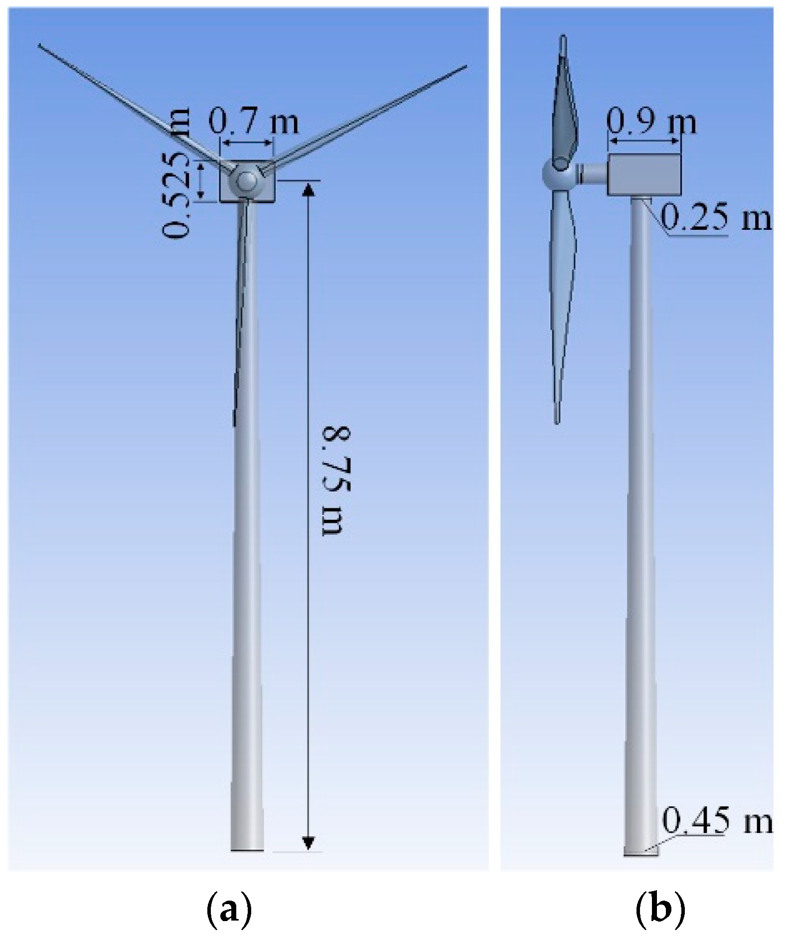
3.1. Geometric Model

The NACA44XX airfoil coordinates are selected in the Profili program. The leaf element coordinates of the blade section are added to the airfoil coordinates. To create the fundamental framework of the blade, the leaf element curves were scaled and rotated around the angle of attack of the airfoil. The laminate surface was used to simulate the leaf element coordinates. The model of the 1.5 MW NREL horizontal axis wind turbine is referenced in the geometric structure. The engine room is a cube structure measuring 0.9 m × 0.7 m × 0.525 m thanks to a simplified design, as shown in Figure 1. The diameter of the wind wheel is 6.5 m, the height of the tower barrel is 8.75 m, the top section diameter of the tower barrel is 0.25 m, and the bottom section diameter is 0.45 m.

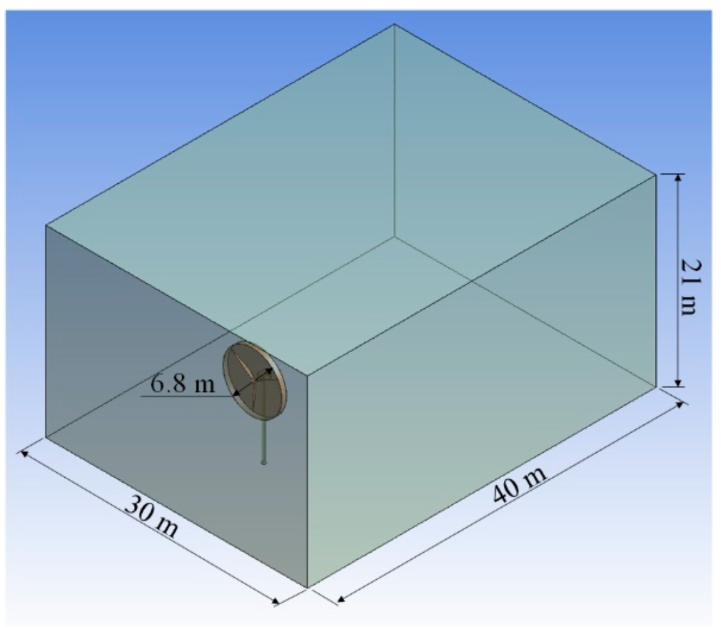
3.2. Computational Domain Configuration

To replicate the wind turbine in its rotating state. The moving cylindrical rotating inner domain enclosing the entire rotor of the wind turbine is joined with the stationary rectangular outer domain containing the engine room and tower barrel. The diameter and thickness of the inner cylinder are 6.8 m and 0.6 m, respectively. By using a Boolean operation, the blade and inner rotation domains are produced. The middle tower and inner basin were removed. In order to simulate the unsteady influence of uniform wind speed and reduce the influence of the boundary environment, the method of digging out the tower cylinder in the outer basin and the inner basin is adopted. The entire calculation area is 40 m × 30 m × 21 m, as shown in Figure 2. The two regions moving relative to each other share a sliding interface that acts as a coupling surface for data transmission.

Before CFD calculation analysis, grid independence verification was carried out. Three different grid sizes were used in the grid test. Grid details and results are shown in

Table 1. Grid details and results.

		Element	Power (kW)
Mesh1	Fine	1,346,994	72.428
Mesh2	Medium	1,084,680	71.431
Mesh3	Coarse	718,140	68.469

. Verify that the grid is divided into fine, medium, and coarse, and the number of grid units increases in equal proportion, and the overall grid growth rate between adjacent grids is 25%. The three grids are simulated and calculated under standard working conditions, and the final output power results are compared. It can be seen that even on the coarse grid, the power difference between the coarse grid and the medium grid is 4.32%, and the power difference between the medium grid and the fine grid is only 1.42%. Therefore, the accuracy of the medium grid is sufficient.

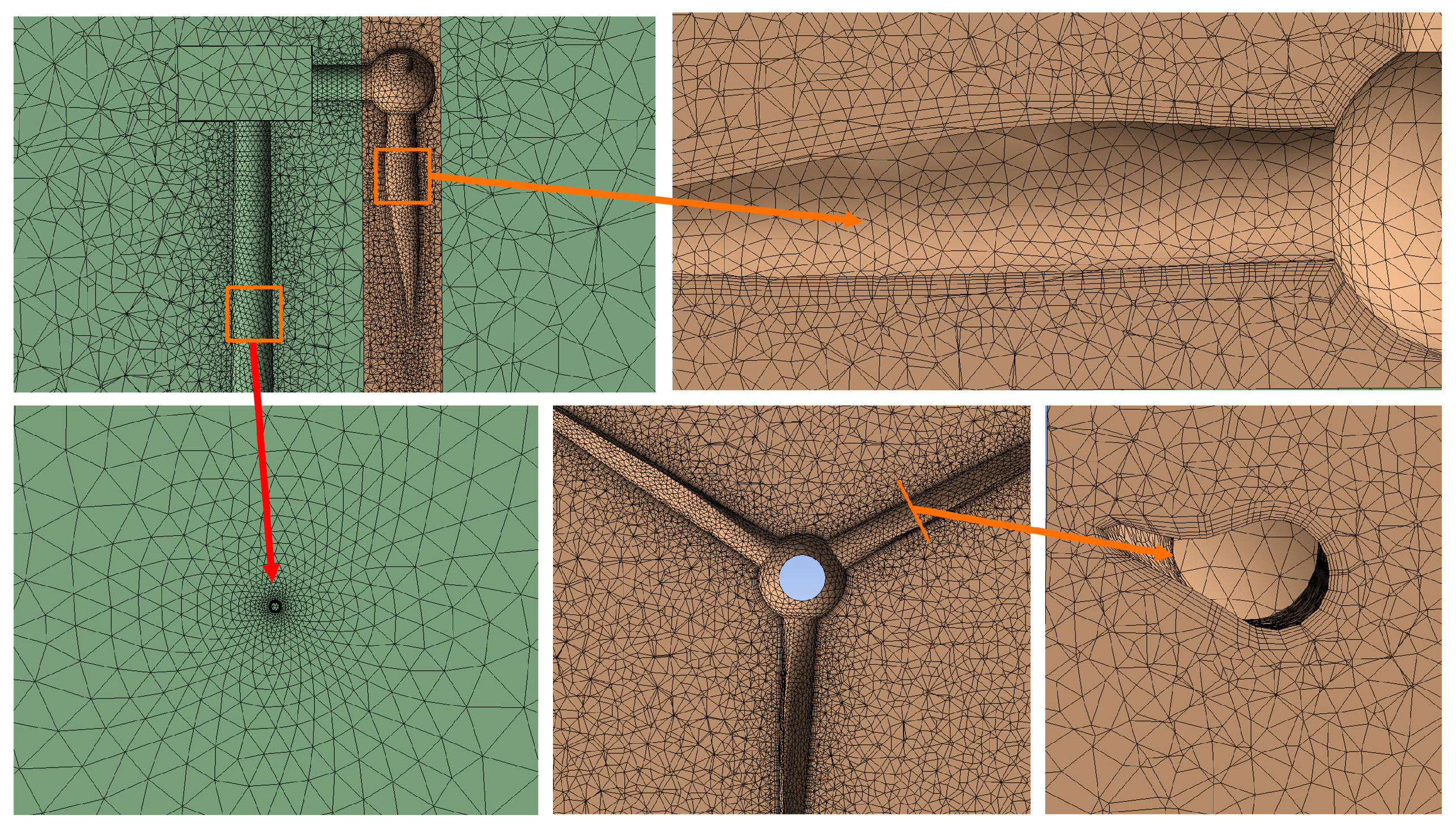
3.2.1. CFD Mesh and Boundary Conditions

The flow field setting is realized by the FLUENT module in ANSYS Workbench. The flow field domain calculation inhibits the structural field part of the overall calculation domain. The blade surface is a rotating wall without slip shear and is also the interface of the fluid domain and the structural domain that transfer data between the two solvers. The area is discretized with unstructured meshes. Finer meshes and additional expansion layers are added to the blade surface to improve resolution. In meshing, the size of the symmetrical wall and ground elements was set at 2.719 m. The size of the volume mesh was set at 0.1 m in the internal rotation domain. The curvature capture division method was adopted, and the normal angle of curvature was defined as 18°. The mesh division of the flow field is shown in Figure 3. The details of the grid’s local magnification are marked in red.

The upstream velocity inlet boundary param was set at free flow wind speed at a distance of 10 m from the entire machine. The initial standard flow rate is 12 m/s, turbulence kinetic energy intensity at 0.05, and turbulence viscosity ratio at 10. A standard atmosphere of pressure is present at the downstream pressure outlet border, which is 30 m from the machine. The fixed symmetric wall surface, ground surface, and blade surface of the inner rotating domain in the outer domain were given non-slip bounds. Frame motion was applied to create the rotation domain to rotate around the Z-axis relative to the stationary domain. As shown in Figure 4, the connection between the wind turbine and the engine room is the rotation axis. The center point of the connection surface is the initial coordinate of the rotation axis. The initial coordinates of the rotation axis were (−4.9567 × 10⁻³, 2.541, 0.7535), and the rotation speed was defined. Since the blade and the rotation domain were in relative motion during the simulation process, a wall motion mode similar to that in the rotation domain was adopted for the blade interface. The moving wall was selected, the movement type was rotation, and the relative speed was 0.

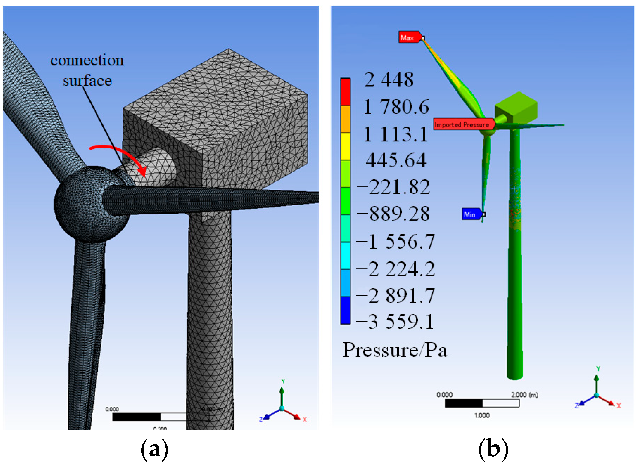
3.2.2. Structural Model Setup

The calculation and setting of the structural field consider the pressure data from the numerical calculation of the flow field and ignore the volume part of the flow field. Before mesh division, material properties are assigned to the wind wheel and tower barrel, respectively, as shown in

Table 2. Wind turbine material properties.

Number	Name	Material	Density (kg/m3)	Young’s Modulus (GPa)	Poisson’s Ratio	Bulk Modulus (GPa)	Shear Modulus (GPa)
1	Blade	Aluminum alloy	2713	69.04	0.33	67.686	25.955
2	Tower	Structure steel	7850	200	0.3	166.67	76.923

.

During blade mesh division, to avoid element distortion at the front and rear flange Angle tips during mesh division, surface mesh division units were embedded, and blade and tower barrel element sizes were set at 0.02 m and 0.05 m, respectively, as shown in Figure 4a. Since the blade surface is a coupled boundary, the aerodynamic force and structural displacement are exchanged, and the large deflection assumption is adopted. The centrifugal force takes into account the rotational speed of the blade structure and defines the rotation mode of the wind wheel. To solve the setting, add the rotation axis and amplitude value of the wind turbine, select the bottom of the wind turbine support, and apply a fixed constraint. In the solution of fluid-structure interaction and structure, the blade surface was taken as the interaction interface, and the flow field pressure data was imported. The maximum pressure value was 2448 Pa, and the minimum pressure value was −3559.1 Pa, as shown in Figure 4b.

4. Results and Discussion

To evaluate the convergence of CFD analysis, the residual, velocity, turbulent kinetic energy, and specific dissipation rate were monitored, 2000 iteration steps were set, the standard initialization method was adopted, and the initial value was calculated from the inlet boundary. The convergence was proved by determining that the residual value was less than 1 × 10⁻⁶ or the net mass percentage was less than 0.1% [39,40]. The result shows that the net export mass flow difference is much less than 0.1% of the total import flow.

4.1. Aerodynamics Distribution

Figure 5 shows the velocity distributions at the wind turbine of z = 1 m plane and the blade, respectively. As plotted in Figure 5a, the global velocity has a range from 0 m/s to 89.25 m/s, and there is a velocity expansion along the blade, in which the velocity increases rapidly from the blade root to the blade tip, and the rotating annular flow pattern can be observed. Considering the blocking effect of the blade structure on the airflow, the area where the blade is rotated forms wind eddy currents, leading to aerodynamic changes. Such eddy currents are generated immediately and disappear quickly with the rotation of the rotor. The vortex alternately and periodically occurs and falls off, dissipating a large amount of energy in the mainstream, so the wind speed in the flow field area where the blade is rotated is lower than that in other areas, which is the reason for the trailing phenomenon of the blade. Figure 5b shows that the hub region is in a relatively static state, and the speed starts to show a linear growth trend at the blade root and gradually develops to the tip at the mid-span.

Figure 6 shows the wind turbine velocity distribution contours at x = 0 m and y = 2.5 m planes. From Figure 6a, it can be seen that the rotation domain is blocked under the incoming wind speed. The velocity variation in the near wind turbine region is concentrated, resulting in wake drag in the downstream region of the wind turbine, and the range of velocity variation expands. Without the barrier of the structure, the airflow exchanges to a steady state. The wind speed of the far wind area along the inflow direction gradually decreases and finally reaches the initial speed. Figure 6b shows that as the wind speed decreases in the flow field created by the wind turbine, the influence range of the airflow disturbance grows steadily bigger. The velocity gradient gradually decreases along the wake region and eventually dissipates in the atmosphere to return to normal wind levels. Due to changes in the adjacent flow field brought on by the tower barrel effect, the distribution position of the tower barrel and engine room, along with the geometric shape of the blades, induce velocity loss in the near wake area, lowering wind speed behind the tower.

Figure 7 shows the pressure distribution contours of the wind turbine rotation domain at the profile z = 1 m and the blade. The pressure of the rotation domain at the profile z = 1 m is shown in Figure 7a. As the wind wheel is shearing the air, negative pressure starts to develop on the lower surface of the blade along the direction of the rotation. The pressure across the middle to the tip of the blade begins to increase. Considering that at the same angular velocity, the linear velocity increases as it stretches along the chord length of the blade. The pressure difference between the upper and lower surfaces of the blade leads to an increase in the airflow supplement exchange speed. It can be observed that the airflow disturbance around the rotation region weakens and tends to be stable with the increase of the radial distance.

The pressure of the blade is shown in Figure 7b. The negative pressure on the upwind surface of the blade ranges from −3160 Pa to −217 Pa. In the middle of the blade, clear negative pressure zones start to form, and negative pressure is concentrated on the blade surface. Additionally, as the blades are propelled by the normal resultant force, the pressure is evenly distributed on the windward. The leeward sides are no longer completely attached to the blade surface due to the action of centrifugal force but instead, eventually dissipate through energy conversion. It complies with the law of energy conservation and also proves the rationality of the aerodynamic characteristics of the wind turbine.

4.2. Structural Response

Figure 8a displays the structural stress contours of a wind turbine during fluid-structure interaction. The analysis reveals that the overall deformation is distributed in a cantilever beam type under fixed support, with the stress primarily concentrating on both sides of the tower barrel. The maximum stress on the top barrel of the blade is eight times greater than on the bottom barrel as it rises steadily from the bottom to the top. The stress at the leading edge of the blade builds in a gradient over the chord length of the airfoil under the assumption of a constant pitch angle.

The wind shear mainly changes the stress gradient on the blade surface. Under the action of clockwise torque, the surface stress on the windward side is greater than that on the leeward side. The minimum stress on the leeward side is 70.058 Pa. The stress concentration area of the wind wheel is located in the area where the blade root is connected to the hub. The stress concentration area is mainly on the mid-span surface of the blade caused by the forward flow shear, and the stress peak value is 5.9239 MPa, which is far less than the designed strength of the blade material.

The strain contours are shown in Figure 8b. The analysis reveals that stress and strain exhibit a linear association because the distribution of the stress-strain contours is essentially the same. The large strain concentration area is located in the middle and upper part of the blade and the middle and lower part of the tower, and the maximum strain is located in the middle and upper part of the blade and reaches 8.6116 × 10⁻⁵ m/m, so the design strength of the middle and upper part of the blade should be improved to prevent fracture. Therefore, the design strength of the upper part of the blade should be improved to prevent breaking.

Figure 9 shows the deformation curve of wind turbine blades during shutdown and rotation. As shown in the lower right corner of Figure 9a, we numbered each blade. The starting point of the displacement curve does not reflect the zero displacement, but the displacement of the blade at the blade root.

The starting points of the three curves represent the displacement of the blade root and are not zero because the displacement on the blade is extracted on the basis of the deformation of the tower barrel, so the initial value corresponds to the displacement value at the top of the tower barrel. The endpoints of the three curves represent the displacement on the tip of the blade. It can be seen from the figure as the position with the largest deformation on the entire blade. The comparative analysis shows that the total displacement curves of the windward side of blade 1 and blade 2 both increase in the positive exponential form under these two conditions. The blade tip deformation is the largest in the shutdown state, and the transverse displacement of the blades in the windward area is basically the same. The same rule applies to rotation conditions.

Under rotating conditions, the response frequency of the blade structure becomes larger, and the overall displacement increases significantly compared with that when the blade is stopped, and the peak increment in the upwind area reaches 2.1437 mm and 0.8674 mm, respectively. It shows that the aerodynamic force and centrifugal force of the wind turbine significantly affect the deformation of the blades during operation. Similarly, the displacement of blade 3 in the downwind area decreases at first and then increases.

Unlike when the blade is stopped, the displacement mutation appears in the second half span and then recovers to the initial value. This is because when the blade overlaps with the tower, the airflow disturbance in the area around the structure is enhanced, and mutual interference leads to the deformation and fluctuation of the blade. When the blade skimmed over the tower, the airflow interference in the interference region was weakened, and the response frequency of the structure began to increase. At this time, the structural response state of blade 3 recovers rapidly until the lower half span begins to show a changing trend similar to the blade deformation in the windward region. It is proved that the azimuth angle has a great influence on the dynamic response of wind turbine structures.

The total deformation change curve of blade 3 in the downwind area of the wind turbine under different speeds is shown in Figure 10. The tower shadow effect affects the structural deformation at standard operating conditions (200 rpm), and the influence of the tower shadow effect on air interference is weakened at lower rotational speeds, resulting in the deformation mutation of the blades in the downwind area being advanced in the structural response. The change of blade deformation at lower rotation speeds (110 rpm, 140 rpm, 170 rpm) is also shown in the figure, and a comparative analysis is made with that at standard speed. The deformation of the blades in the downwind region also has a similar mutation as that under the standard speed, resulting in an advance in the structural response of the blades in the downwind region. The most intuitive representation in the figure is the advance of the deformation mutation point in the upward diffusion process of the blade. At lower rotational speeds, the influence of the tower shadow effect on air interference is enhanced, making it more difficult to get rid of the influence of tower shadow downwind. When the rotational speed increases, the deformation of the blades in the downwind region develops towards the blades in the upwind region, resulting in the mutation point moving toward the blade tip.

4.3. Torque and Output Power

To study the output power changes of wind turbines with different wind speeds under uniform inflow conditions, the inflow conditions were set at 5 m/s, 8 m/s, 10 m/s, 12 m/s, 15 m/s, 18 m/s, and 20 m/s. The above inflow conditions were simulated and calculated, respectively, and the wind turbine torque value M under different working conditions was obtained through data processing. The wind turbine output power P was obtained by using the following formula, and then the output data was analyzed.

$$P=M\omega$$

(10)

where, $\omega$ is the angular velocity, $\omega =\mathrm{RPM}·\pi /30$, rad/s.

Figure 11 shows the variation curve of wind turbine output power under different incoming flow conditions.

It can be concluded from the figure above that the output power of the wind turbine presents approximately linear changes under different uniform inlet flows of the wind field. When the inlet wind speed increases from 5 m/s to 20 m/s, the output power of the wind turbine increases from 68.33 kW to 84.33 kW, respectively. In the process of increasing output power, considering that the torque of wind turbines increases with the increase of windward speed. The aerodynamic pressure captured by wind turbine blades under the larger inlet wind speed is also higher. Due to the structural characteristics of the blades, under the action of the flow field, blade surface load changes blade shape param, and the lift-drag ratio of wind turbines increases. This results in better performance of the blades and an increase in output power.

The wind energy captured in the operation of wind turbines is provided to the rotor to generate torque. The centrifugal force diffuses the flow field data to the surrounding area, enhances the interaction of wind speed, and increases the central torque of wind turbines. Such changes in radial flow velocity and pressure are more significant, and ultimately, the output power is generated in essence. The mechanical properties of wind turbine blade speed and pressure are different under different wind conditions, which provides topic guidance for the study of wind turbine overall aerodynamic performance or aerodynamics.

The output power increases linearly with the incoming flow speed, and there is a strong correlation between the two. It is conceivable that this variation may represent the general characteristics of wind turbines at real-time wind speeds. In addition,

Table 3. CFD models are derived from the previous sources of literature.

Literature Source	Geometric Parameter	Turbulence Model	Incoming Velocity (m/s)	R2
Wang et al. [26]	100 m × 82 m × 50 m	k–ω SST	7.0–20.0	0.98736
Mo et al. [38]	90.6 m × 45.3 m × 90.6 m	k–ω SST	7.0–25.1	0.95218
Liu et al. [41]	24.4 m × 36.6 m	one−equation SpalarteAllmaras	7.0–20.0	0.96923

and Figure 12 show three previous studies [26,38,41] for power monitoring under changes in wind speed under different model sizes and turbulence models. The parameter values and results of similar CFD models under different studies are shown in Table 3, and the variation trend of the standardized power of the literature model with the standardization speed is shown in Figure 12. The velocity curves of the standardized calculation results of the three similar studies are also similar to those in this paper.

Wang et al. [26] and Liu et al. [41] are consistent with the variation range of incoming wind speed in this paper, but the CFD turbulence model adopted by them is different. The standardized power variation of the two models has a good correlation with the standardized speed, and the fitting correlation is relatively consistent with the CFD calculation results of the k–ω SST model in this paper. While the wind speed range of Mo et al. [38] is large, although the R² value is small, the results still confirm that the power has good growth at lower wind speeds. There is also a basically consistent trend of change. Compared with the CFD results of Wang et al. [26], Mo et al. [38], and Liu et al. [41], it can be seen that this study has a good similar variation rule with the literature data. It confirms the reliability of the CFD results and model.

5. Conclusions

The finite element software ANSYS is used to study the downstream solid interaction aerodynamic characteristics of wind turbines under the action of the flow field, and the following conclusions are drawn.

(1)

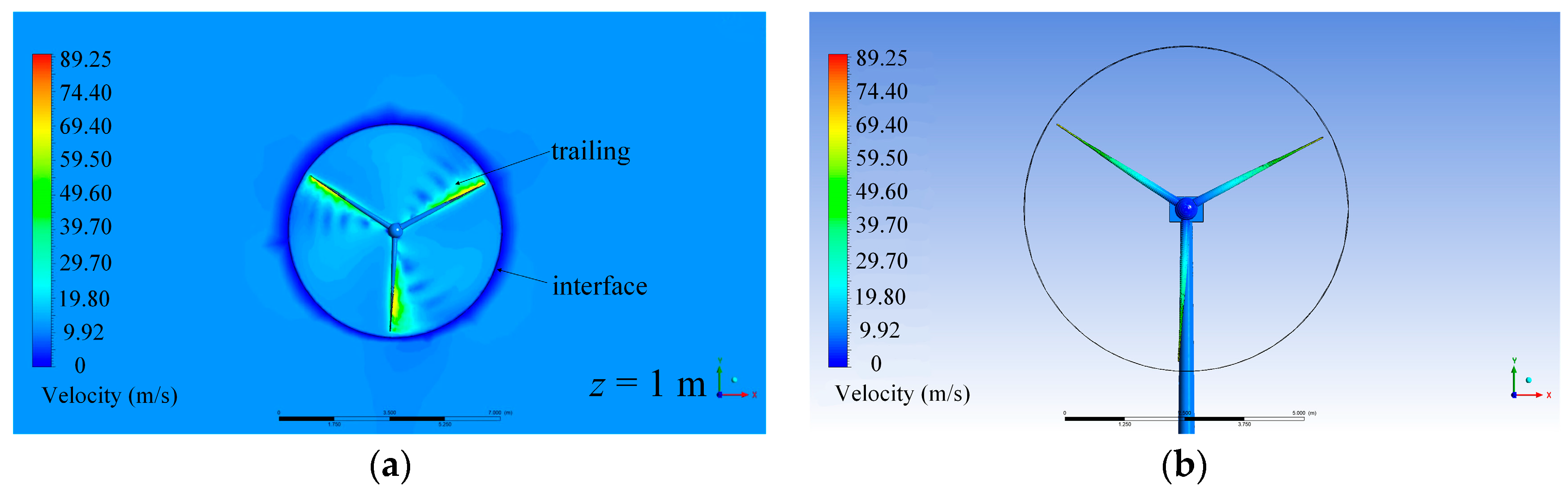
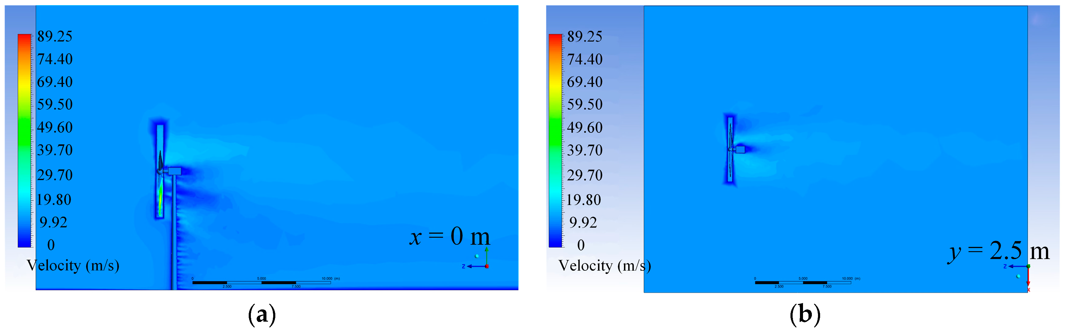
The fluid-structure interaction wind field model of the wind turbine is established and verified in light of the complexity of the aerodynamic environment. Under the influence of inflow wind and rotation in the flow field, the airflow disturbance closest to the wind turbine is the most important. Under the interference of the tower shadow effect, the wind speed in the near wake zone and the far wake zone decreases to varying degrees along the incoming wind direction.

(2)

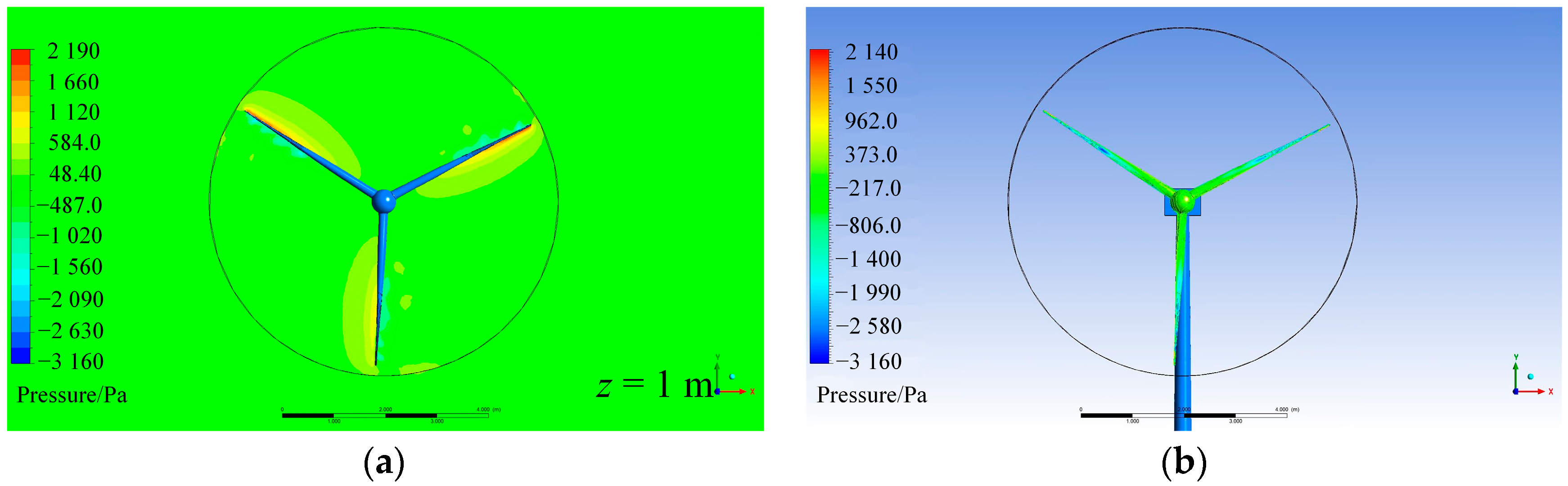
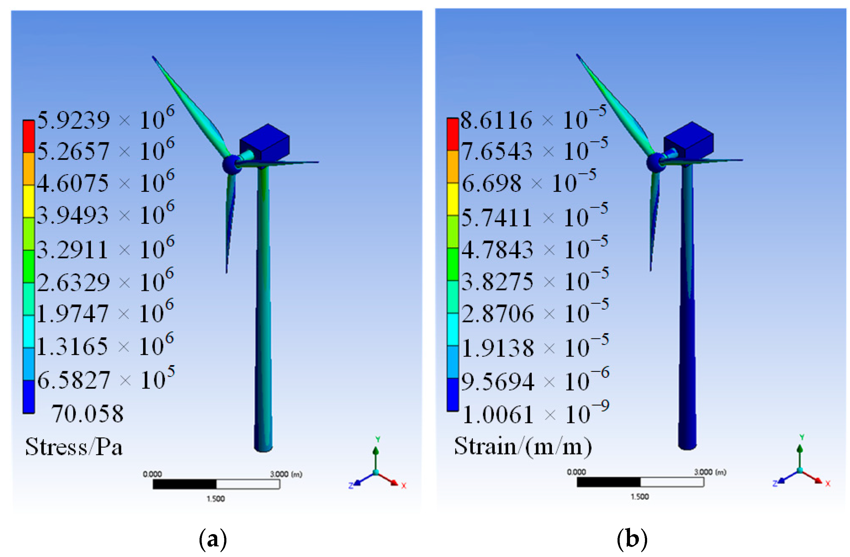
While the centrifugal force of the normal force that drives the pressure around the wind turbine has a greater impact and the pressure around the wind turbine changes primarily along the radial direction with the weakening of the airflow disturbance, the windward side of the blade first experiences the action of airflow, and the pressure changes in a wide range. The maximum stress in the structural reaction of the tower is eight times greater at its top than it is at its bottom. The peak blade stress reaches 5.92 MPa.

(3)

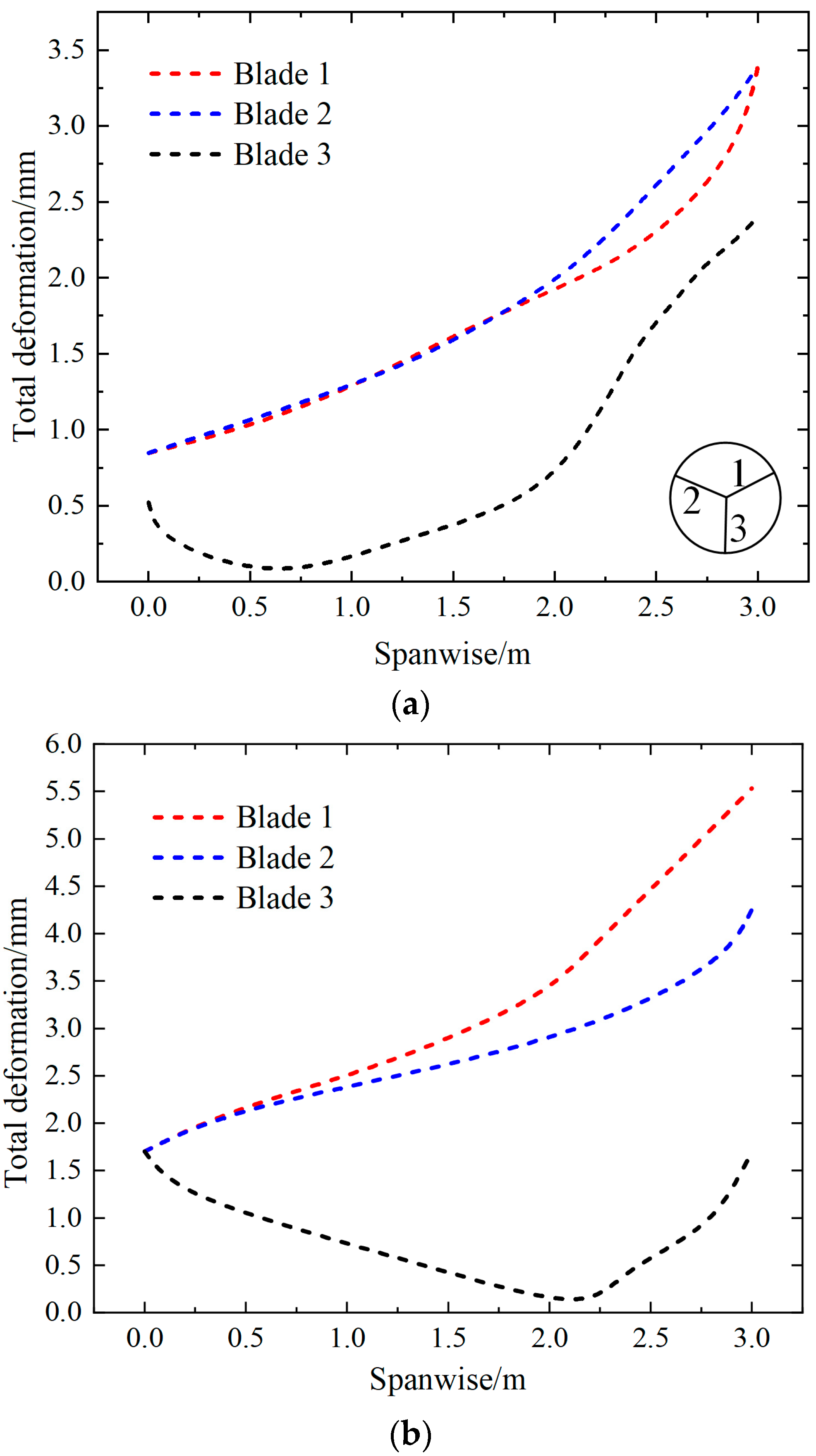
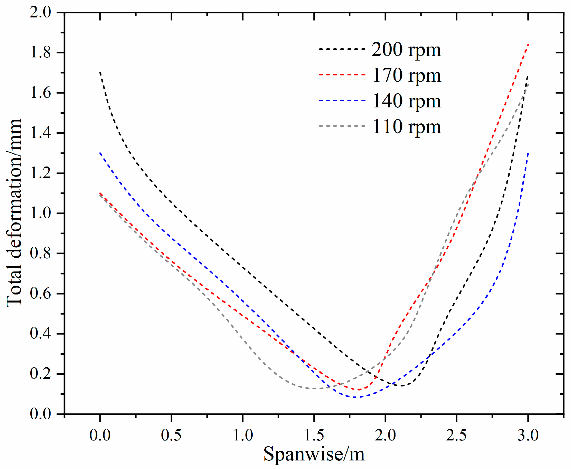
The change in wind turbine blade displacement in the upwind direction under standard (12 m/s and 200 rpm) and shutdown conditions is the same and grows exponentially. Under the action of rotation, the transverse deformation of blade 3 occurred in 73%, and the transverse deformation of downwind blade 3 was almost unchanged at 20%. With the increase of wind turbine speed, the abrupt deformation point of the blade in the downwind area moves towards the blade tip.

(4)

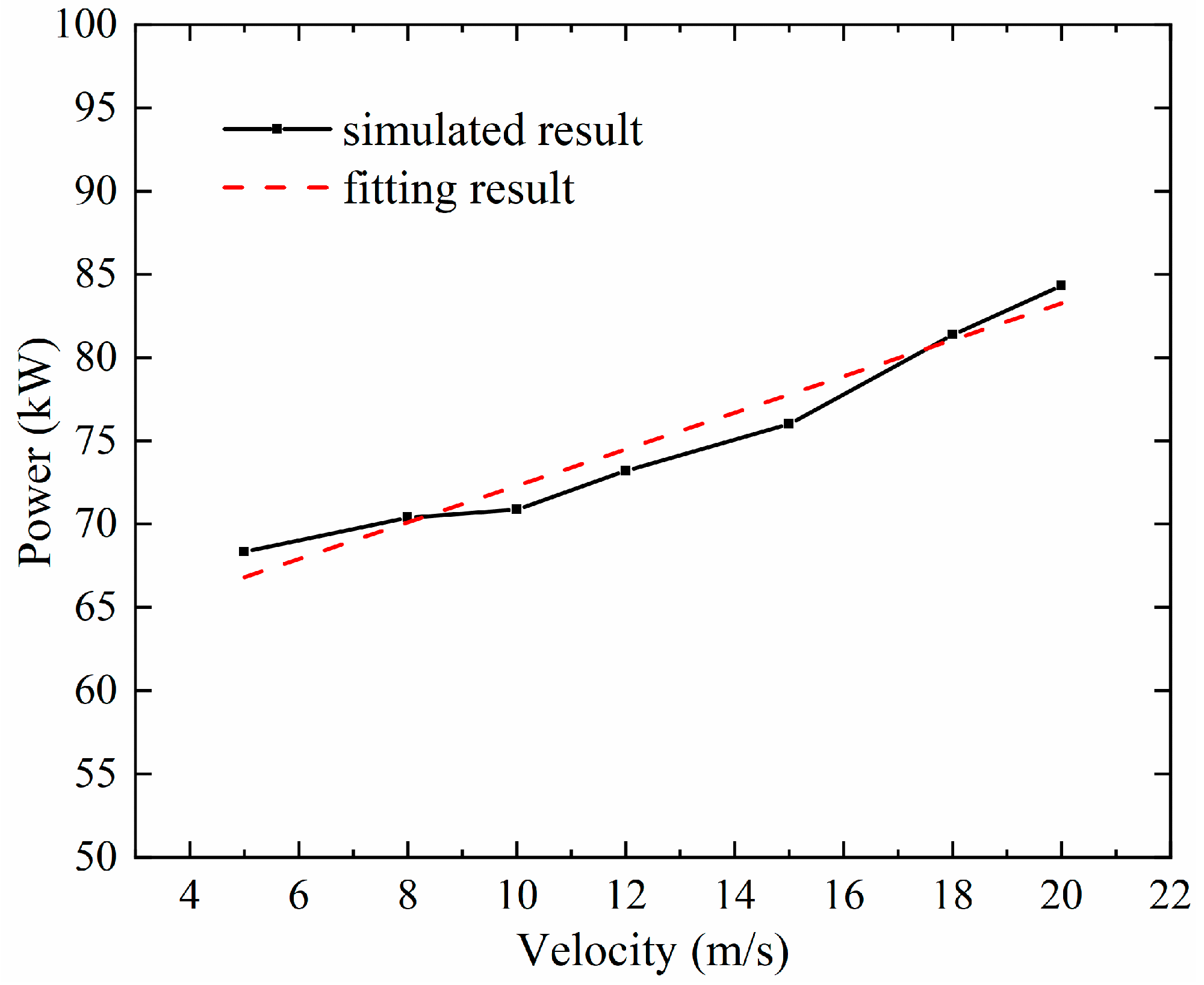
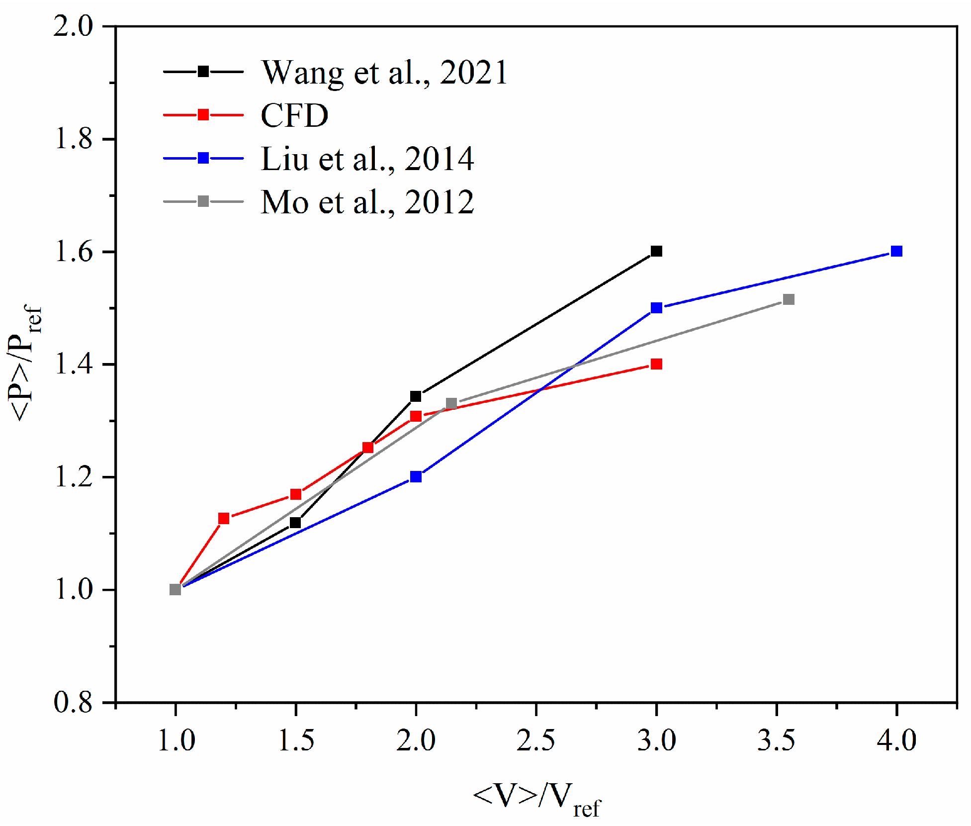
The aerodynamic impact of the wind turbine is improved by increasing the entering wind speed, catching more wind energy, producing a considerable bending moment and power, and increasing output power by a net 20 kW.

References

1. Global Wind Energy Council. GWEC Global Wind Report; Global Wind Energy Council: Brussels, Belgium, 2021. [Google Scholar]
2. Dai, K.; Bergot, A.; Liang, C.; Xiang, W.N.; Huang, Z. Environmental issues associated with wind energy—A review. Renew. Energy 2015, 75, 911–921. [Google Scholar] [CrossRef]
3. Fridleifsson, I.B. Geothermal energy for the benefit of the people. Renew. Sustain. Energy Rev. 2001, 5, 299–312. [Google Scholar] [CrossRef]
4. Gebhardt, C.G.; Preidikman, S.; Massa, J.C. Numerical simulations of the aerodynamic behavior of large horizontal-axis wind turbines. Int. J. Hydrog. Energy 2010, 35, 6005–6011. [Google Scholar] [CrossRef]
5. Cai, X.; Gu, R.; Pan, P.; Zhu, J. Unsteady aerodynamics simulation of a full-scale horizontal axis wind turbine using CFD methodology. Energy Convers. Manag. 2016, 112, 146–156. [Google Scholar] [CrossRef]
6. AbdelSalam, A.M.; Ramalingam, V. Wake prediction of horizontal-axis wind turbine using full-rotor modeling. J. Wind Eng. Ind. Aerodyn. 2014, 124, 7–19. [Google Scholar] [CrossRef]
7. Almohammadi, K.M.; Ingham, D.B.; Ma, L.; Pourkashan, M. Computational fluid dynamics (CFD) mesh independency techniques for a straight blade vertical axis wind turbine. Energy 2013, 58, 483–493. [Google Scholar] [CrossRef]
8. Danao, L.A.; Edwards, J.; Eboibi, O.; Howell, R. A numerical investigation into the influence of unsteady wind on the performance and aerodynamics of a vertical axis wind turbine. Appl. Energy 2014, 116, 111–124. [Google Scholar] [CrossRef]
9. Leishman, J.G. Challenges in modelling the unsteady aerodynamics of wind turbines. Wind Energy 2002, 5, 85–132. [Google Scholar] [CrossRef]
10. Li, Y.; Guo, X.; Li, R.; Li, D.; Dong, Y.; Zhao, L. Unsteady characteristics of pressure on wind turbine blade surface in the field. Mod. Phys. Lett. B 2021, 35, 2150281. [Google Scholar] [CrossRef]
11. Liu, P.; Yu, G.; Zhu, X.; Du, Z. Unsteady aerodynamic prediction for dynamic stall of wind turbine airfoils with the reduced order modeling. Renew. Energy 2014, 69, 402–409. [Google Scholar] [CrossRef]
12. Schepers, J.G.; Boorsma, K.; Cho, T.; Gomez-Iradi, S.; Schaffarczyk, P.; Jeromin, A.; Shen, W.Z.; Lutz, T.; Meister, K.; Stoevesandt, B.; et al. Analysis of Mexico Wind Tunnel Measurements: Final Report of IEA Task 29, Mexnext (Phase 1). 2012, Energy Research Centre of The Netherlands (ECN). ECN-E No. 12-004. Available online: https://orbit.dtu.dk/en/publications/analysis-of-mexico-wind-tunnel-measurements-final-report-of-iea-t (accessed on 13 July 2023).
13. Zhang, L.; Li, X.; Li, S.; Bai, J.; Xu, J. Unstable aerodynamic performance of a very thick wind turbine airfoil CAS-W1-450. Renew. Energy 2019, 132, 1112–1120. [Google Scholar] [CrossRef]
14. Bai, C.J.; Wang, W.C. Review of computational and experimental approaches to analysis of aerodynamic performance in horizontal-axis wind turbines (HAWTs). Renew. Sustain. Energy Rev. 2016, 63, 506–519. [Google Scholar] [CrossRef]
15. Cao, L.; Sun, W.; Zhou, J.; Cui, Q. Dynamic performance analysis for wind turbine in complex conditions. J. Vibroeng. 2020, 22, 209–224. [Google Scholar] [CrossRef]
16. Lee, Y.J.; Jhan, Y.T.; Chung, C.H. Fluid-structure interaction of FRP wind turbine blades under aerodynamic effect. Compos. Part B Eng. 2012, 43, 2180–2191. [Google Scholar] [CrossRef]
17. Li, Y.; Castro, A.M.; Sinokrot, T.; Prescott, W.; Carrica, P.M. Coupled multi-body dynamics and CFD for wind turbine simulation including explicit wind turbulence. Renew. Energy 2015, 76, 338–361. [Google Scholar] [CrossRef]
18. Wang, Y.; Li, G.; Shen, S.; Huang, D.; Zheng, Z. Investigation on aerodynamic performance of horizontal axis wind turbine by setting micro-cylinder in front of the blade leading edge. Energy 2018, 143, 1107–1124. [Google Scholar] [CrossRef]
19. Regodeseves, P.G.; Morros, C.S. Unsteady numerical investigation of the full geometry of a horizontal axis wind turbine: Flow through the rotor and wake. Energy 2020, 202, 117674. [Google Scholar] [CrossRef]
20. Vaz, J.R.P.; Pinho, J.T.; Mesquita, A.L.A. An extension of BEM method applied to horizontal-axis wind turbine design. Renew. Energy 2011, 36, 1734–1740. [Google Scholar] [CrossRef]
21. Kim, Y.; Bangga, G.; Delgado, A. Investigations of HAWT Airfoil Shape Characteristics and 3D Rotational Augmentation Sensitivity toward the Aerodynamic Performance Improvement. Sustainability 2020, 12, 7957. [Google Scholar] [CrossRef]
22. Mdouki, R. Parametric study of magnus wind turbine with spiral fins using BEM approach. J. Appl. Fluid Mech. 2021, 14, 887–895. [Google Scholar]
23. Dumitrescu, H.; Cardos, V. Wind Turbine Aerodynamic Performance by Lifting Line Method. Int. J. Rotating Mach. 1998, 4, 141–149. [Google Scholar] [CrossRef]
24. Coton, F.N.; Wang, T. The prediction of horizontal axis wind turbine performance in yawed flow using an unsteady prescribed wake model. Proc. Inst. Mech. Eng. Part A J. Power Energy 1999, 213, 33–43. [Google Scholar] [CrossRef]
25. Moon, H.G.; Park, S.; Ha, K.; Jeong, J.H. CFD-based in-depth investigation of the effects of the shape and layout of a vortex generator on the aerodynamic performance of a multi-MW wind turbine. Appl. Sci. 2021, 11, 10764. [Google Scholar] [CrossRef]
26. Wang, Y.; Wang, L.; Duan, C.; Zheng, J.; Liu, Z.; Ma, G. CFD simulation on wind turbine blades with leading edge erosion. J. Theor. Appl. Mech. 2021, 59, 579–593. [Google Scholar] [CrossRef]
27. Khan, S.; Li, M.S. A modeling study focused on improving the aerodynamic performance of a small horizontal-axis wind turbine. Sustainability 2023, 15, 5506. [Google Scholar] [CrossRef]
28. Oliveira, H.A.; de Matos, J.G.; Ribeiro, L.A.D.S.; Saavedra, O.R.; Vaz, J.R.P. Assessment of Correction Methods Applied to BEMT for Predicting Performance of Horizontal-Axis Wind Turbines. Sustainability 2023, 15, 7021. [Google Scholar] [CrossRef]
29. Madsen, H.A.; Riziotis, V.; Zahle, F.; Hansen, M.; Snel, H.; Grasso, F.; Larsen, T.; Politis, E.; Rasmussen, F. Blade element momentum modeling of inflow with shear in comparison with advanced model results. Wind Energy 2012, 15, 63–81. [Google Scholar] [CrossRef]
30. Sang, S.; Wen, H.; Cao, A.X.; Du, X.R.; Zhu, X.; Shi, Q.; Qiu, C.H. Dynamic modification method for BEM of wind turbine considering the joint action of installation angle and structural pendulum motion. Ocean Eng. 2020, 215, 107528. [Google Scholar] [CrossRef]
31. Dong, J.; Viré, A.; Ferreira, C.S.; Li, Z.; Van Bussel, G. A modified free wake vortex ring method for horizontal-axis wind turbines. Energies 2019, 12, 3900. [Google Scholar] [CrossRef]
32. Shaler, K.; Kecskemety, K.M.; McNamara, J.J. Benchmarking of a free vortex wake model for prediction of wake interactions. Renew. Energy 2019, 136, 607–620. [Google Scholar] [CrossRef]
33. Andreopoulos, W.Y. Density and compressibility effects in turbulent subsonic jets part 1: Mean velocity field. Exp. Fluids 2010, 48, 327–343. [Google Scholar]
34. Menter, F.R. Two-equation eddy-viscosity turbulence models for engineering applications. AIAA J. 1994, 32, 1598–1605. [Google Scholar] [CrossRef]
35. Wilcox, D.C. Formulation of the k-omega turbulence model revisited. AIAA J. 2008, 46, 2823–2838. [Google Scholar] [CrossRef]
36. Jones, W.P.; Launder, B.E. The prediction of laminarization with a two-equation model of turbulence. Int. J. Heat Mass Transf. 1972, 15, 301–314. [Google Scholar] [CrossRef]
37. Johansen, J.; Sørensen, N.N.; Michelsen, J.A.; Schreck, S. Detached-eddy simulation of flow around the NREL Phase-VI rotor. Wind Energy 2002, 5, 185–197. [Google Scholar] [CrossRef]
38. Mo, J.O.; Lee, Y.H. CFD Investigation on the aerodynamic characteristics of a small-sized wind turbine of NREL PHASE VI operating with a stall-regulated method. J. Mech. Sci. Technol. 2012, 26, 81–92. [Google Scholar] [CrossRef]
39. Bourdin, P.; Wilson, J.D. Windbreak aerodynamics: Is computational fluid dynamics reliable? Bound. Layer Meteorol. 2008, 126, 181–208. [Google Scholar] [CrossRef]
40. Wang, L.; Quant, R.; Kolios, A. Fluid structure interaction modelling of horizontal-axis wind turbine blades based on CFD and FEA. J. Wind Eng. Ind. Aerodyn. 2016, 158, 11–25. [Google Scholar] [CrossRef]
41. Liu, Z.Y.; Wang, X.D.; Kang, S. Stochastic performance evaluation of horizontal axis wind turbine blades using non-deterministic CFD simulations. Energy 2014, 73, 126–136. [Google Scholar] [CrossRef]
Figure 1. Wind turbine full-scale model. (a) front view; (b) side view.
Sustainability 15 12553 g001
Figure 2. Diagram of the computational domain for wind turbines.
Sustainability 15 12553 g002
Figure 3. Boundary layer detail mesh in the fluid domain.
Sustainability 15 12553 g003
Figure 4. (a) Structural mesh model; (b) Aerodynamic load loading.
Sustainability 15 12553 g004
Figure 5. The velocity contours at (a) wind turbine of z = 1 m plane and (b) wind turbine blade.
Sustainability 15 12553 g005
Figure 6. The plane flow field velocity contours at (a) x = 0 and (b) y = 2.5 m.
Sustainability 15 12553 g006
Figure 7. Pressure contours in the (a) rotational domain and (b) surface of the rotor.
Sustainability 15 12553 g007
Figure 8. (a) stress contours; (b) strain contours.
Sustainability 15 12553 g008
Figure 9. Blade deformation under (a) shutdown condition and (b) rotating operating condition.
Sustainability 15 12553 g009
Figure 10. Total deformation of the downwind zone at different speeds.
Sustainability 15 12553 g010
Figure 11. Variation of output power under different incoming streams.
Sustainability 15 12553 g011
Figure 12. Comparison of standardized power variation in the sources of literature of Wang et al. [26], Mo et al. [38] and Liu et al. [41].
Sustainability 15 12553 g012