Intrusion Detection in Healthcare 4.0 Internet of Things Systems via Metaheuristics Optimized Machine Learning

Abstract

Rapid developments in Internet of Things (IoT) systems have led to a wide integration of such systems into everyday life. Systems for active real-time monitoring are especially useful in areas where rapid action can have a significant impact on outcomes such as healthcare. However, a major challenge persists within IoT that limit wider integration. Sustainable healthcare supported by the IoT must provide organized healthcare to the population, without compromising the environment. Security plays a major role in the sustainability of IoT systems, therefore detecting and taking timely action is one step in overcoming the sustainability challenges. This work tackles security challenges head-on through the use of machine learning algorithms optimized via a modified Firefly algorithm for detecting security issues in IoT devices used for Healthcare 4.0. Metaheuristic solutions have contributed to sustainability in various areas as they can solve nondeterministic polynomial time-hard problem (NP-hard) problems in realistic time and with accuracy which are paramount for sustainable systems in any sector and especially in healthcare. Experiments on a synthetic dataset generated by an advanced configuration tool for IoT structures are performed. Also, multiple well-known machine learning models were used and optimized by introducing modified firefly metaheuristics. The best models have been subjected to SHapley Additive exPlanations (SHAP) analysis to determine the factors that contribute to occurring issues. Conclusions from all the performed testing and comparisons indicate significant improvements in the formulated problem.

1. Introduction

Healthcare 4.0 [1] is essentially a concept that can be considered to be a part of the Fourth Industrial Revolution, and it can be implemented by utilizing technologies such as artificial intelligence (AI), IoT, data analytics, and many others. This concept is crucial for overall improvement in the healthcare industry, enabling better accessibility, enhancing quality, and ensuring high efficiency in healthcare treatment [1]. By using this concept, the integration of personalized medicine is achieved, and smart patient care devices can be implemented, along with remote healthcare delivery solutions which are all paramount to achieving a sustainable healthcare system. Advanced technologies like Healthcare 4.0 can have certain challenges, particularly in terms of data security and privacy [2], which hinder its adoption rate. The primary concern revolves around protecting user data [3], which contains sensitive information about the service user or patient. The data stored in the database is of an extremely sensitive nature, encompassing personal information such as the user’s genetic code, medical history, identification details, and many others. Additionally, the lack of standards within this concept poses integration issues with various systems. Introducing standards can improve the mechanism of data exchange among different device levels and facilitate resource sharing among relevant healthcare institutions.

An important aspect of the Healthcare 4.0 concept which heavily influences sustainability is the provision of real-time information, aiming to enable faster and more efficient responses from medical staff and doctors, thereby achieving more effective patient diagnoses [1]. At any given moment, doctors have access to data indicating the current condition of the patient. It is also noteworthy that vital patient parameters can be monitored live, in real time [4]. In the event of deviations from the defined parameters set by the doctor, the medical staff and the doctor can immediately change the therapy and provide the appropriate treatment. Additionally, the Healthcare 4.0 concept facilitates the efficiency of detecting emergency cases, such as a heart attack in a patient. In such cases, appropriate measures are taken to save the patient’s life. The technology of Healthcare 4.0 can facilitate consultations with doctors in relevant medical fields, allowing for a more efficient exchange of necessary information with relevant medical institutions. This enables faster medical decision-making based on real-time diagnostics. The influence on sustainable cities is present in Healthcare 4.0 as well. Route optimization is important for sustainable health service providing which intertwines with other concepts like smart and sustainable cities. There is more on this topic in Section 2, which provides the literature review.

Every technology in the world has its vulnerabilities, and Healthcare 4.0 [3], with the use of the IoT, also faces issues regarding data protection and integrity. One of the attack techniques present in this technology is the man-in-the-middle attack, where patient data are intercepted. Furthermore, due to the use of weaker data encryption techniques [5] in the exchange of data between patients and relevant institutions on IoT devices, unauthorized access to sensitive and personal patient information can occur. Computer networks and systems that have IoT devices and integrated Healthcare 4.0 technology on their servers can be susceptible to potential attacks on the network infrastructure, where attackers intentionally attempt to disrupt the use of active services. Such attacks can cause damage to the network infrastructure or render it completely incapacitated [6,7]. As a result of such attacks, the attacker can install malicious software on devices, aiming to target IoT devices that interact with patients. The reason for these attacks is unauthorized access to patient data, where even solutions like blockchain are combined with IoT structures [8]. In addition to the proper training of employees regarding potential data leaks, where the human factor often plays a significant role, possible protection against such attacks can be the implementation and integration of hardware and software firewall mechanisms, as well as the implementation of the intrusion detection system (IDS) and intrusion prevention system (IPS) [9]. The implementation of IDS/IPS systems is of great importance to detect any suspicious activity in computer networks or cloud systems where Healthcare 4.0 technology is implemented in a timely manner [9]. Conclusively, a sustainable health system is not possible without ensuring a stable and secure infrastructure which is challenging as is due to a large number of device types and devices in general.

Healthcare 4.0 technology requires the implementation of mechanisms that can adapt to new potential vulnerabilities. In addition to the previously mentioned systems, other technologies can be utilized, such as automated incident response systems, security analytics systems, and identity and access management systems. Furthermore, a vulnerability management system can be employed to identify issues and detect vulnerabilities within the infrastructure of computer networks or cloud systems.

Artificial intelligence holds great potential in addressing numerous vulnerabilities and overall security challenges faced by Healthcare 4.0 technology. AI can utilize advanced machine learning algorithms to analyze large datasets and draw conclusions about potential threats or attacks. From such data sets, it is possible to identify patterns that may indicate a threat or attack. Moreover, based on such analyses, AI can discover and detect new potential system vulnerabilities that may appear unusual to the implemented systems. By leveraging known vulnerabilities, AI can even predict or anticipate attacks in advance.

Advanced machine learning algorithms can predict or take preventive measures before an actual infrastructure attack occurs. Through automation, efficiency can be achieved by implementing automated incident response in the infrastructure [9]. In the event of an attack or the introduction of malicious code into the infrastructure, AI can recognize attack patterns and automatically respond to them [9].

When it comes to data within the infrastructure where user data are stored, AI can enhance encryption mechanisms using deep learning on existing encryption algorithms. This improves the existing data encryption technique, and through deep learning, vulnerability detection mechanisms and systems can be enhanced, resulting in more modern data encryption systems being produced automatically.

To achieve sustainable environments and higher quality of life, it is paramount to take into account all the different aspects of the healthcare systems that are not universal around the globe. Researchers explore topics like the supply chains of pharmaceuticals [10], combine technologies like blockchain with IoT infrastructure for the optimized road health assistance [11], and even topics that do not affect the patient directly but electricity management in a hospital can bring other types of quality of service improvements and increase the well-being of patients leading the society to a more sustainable world [12].

Extreme gradient boosting (XGBoost) is an algorithm that has proven to be the best optimizer for competition. It is a gradient-boosting-based approach that increases the learner’s performance and reduces bias and even variance. It is considered a tree-based algorithm due to its foundation being strongly related to it. Due to the complicated process of hyperparameter optimization, XGBoost is paired with an optimizer.

Metaheuristic optimization is recognized to be on the rise because of the high-performance outputs that can be achieved. The advantage of such solutions comes from their NP hard-solving capabilities. The need for extensive experimentation in this field comes from the no free lunch (NFL) theorem, and according to it, no single solution is equally good for solving all problems [13].

The authors have chosen the firefly algorithm (FA) metaheuristic based on swarm behavior as a method for optimization due to its history of high performance for NP-hard optimization. Even though they are powerful optimizers, swarm intelligence (SI) algorithms are not without shortcomings. Where one algorithm excels, another fails. Hence, the authors apply modifications to the original solution, proposing a modified firefly algorithm (MFA) with superior performance to the original solution as well as to all the compared metaheuristics. The predictions were performed with the XGBoost technique, which is optimized by the MFA. A synthetic dataset was used for testing, but note that the dataset was generated by a powerful tool that allows for virtually any scenario setup. Finally, to further elaborate on the performance of the proposed method, the authors provide a SHAP analysis.

The main contributions of this work include a robust system for security breach detection for the use case of IoT in healthcare, the proposition of a modified metaheuristic algorithm with improved performance, and a study case on the generated IoT traffic dataset.

• A robust healthcare security system based on the XGBoost technique optimized by the proposed MFA.
• Modification proposals for the FA swarm metaheuristic.
• Improvements validated through extensive testing on a simulated dataset with comparison to eight other XGBoost-metaheuristic optimized solutions.
• Performance optimization based on the SHAP feature importance which clearly indicates which features contribute to which predicted class.
• Best performance interpretation using SHAP analysis for better transparency.

The structure of the manuscript is as follows: Section 2 refers to the fundamentals of this research and similar work, Section 3 provide the original algorithm and modifications applied to it, Section 4 describes the used dataset, experimental setup, and employed metrics, Section 5 describes the obtained results, and Section 6 provides a summarization of this work and future work propositions.

2. Background and Preliminaries

2.1. Literature Review

More and more devices IoT are being connected to traditional computer networks. Such networks are commonly referred to as IoT networks. The security of the IoT ecosystem is based on safeguarding sensitive user data, given that IoT devices are finding increasing applications in all spheres of modern life. Data are typically outsourced and stored on remote cloud servers, which are also accessed by IoT devices. As these devices can generate a large amount of sensitive data, it is essential to enhance comprehensive protection [14].

The latest advancements in the field of IoT are being analyzed, and it is necessary to enhance them by utilizing AI and deep learning [15]. It has been emphasized that technological challenges and gaps have been identified in the IoT-based cloud infrastructure, and it is crucial to improve the entire domain [15].

Hathaliya et al. [2] conducted an interesting study, providing an overview of the transformation from Healthcare 1.0 to 4.0. They emphasized that insecure Healthcare 4.0 techniques can lead to privacy breaches of health data. Attackers can gain access to sensitive information such as user email accounts, patient health reports, exchanged messages with relevant parties, and more. Additionally, the authors found that this technology can also achieve success in terms of data exchange efficiency. Thamilarasu et al. [16] were able to achieve high detection accuracy with minimal resource overhead through simulations. They successfully contributed to improving the overall security of IoT devices used by patients by using simulations to mitigate potential attacks.

The scientific paper [17] explores the problem of vulnerability and security in IoT devices, with a focus on the healthcare domain. The authors have determined that, even with a well-organized network infrastructure using traditional approaches, existing protection mechanisms cannot directly guarantee the security of IoT devices against cyber-attacks due to resource limitations and specific IoT protocols. The authors have proposed a new framework for developing a novel solution for contextual security of IoT devices to facilitate the detection of attacks on the network infrastructure. For the purposes of the study, the authors have utilized a newly developed open-source tool called IoT-Flock for generating IoT data. This tool enabled the authors to develop scenarios that can generate normal and malicious traffic. The outcome of the study resulted in the proposal of a new framework for contextual security of IoT devices and highly sensitive scenarios, such as the IoT healthcare environment.

Hussain et al. [18] focused on the impact of IoT on modern life in various domains. Due to limited resources, IoT devices are attractive targets for cyber-attacks. The paper highlights that traditional encryption methods are not sufficient to protect data integrity in IoT networks, so the authors utilized machine learning and deep learning techniques to enhance security. The authors of the paper [19] focused their research on the development of intelligent components for the identification and profiling of IoT devices, as well as the detection of intrusions in complex IoT network environments. For authentication purposes, the authors proposed fingerprinting techniques. For the needs of the study, the authors created a laboratory environment where they collected data based on four states of each device: on, idle, active, and interaction. In addition to this, the authors simulated smart home activities. Two sets of data were also generated: denial of service (DoS) attacks and brute-force attacks on real time streaming protocol (RTSP) protocols. The authors aimed to create a reference IoT dataset that is realistic and can contribute to and enhance future research in terms of training and evaluating intelligent components of IoT systems, where identification, profiling, and potential intrusion detection need to be performed. The research of this paper revolves around the hypothesis that emphasizes the significance of security in healthcare for sustainability, where data security and integrity play a crucial role. Additionally, the datasets and algorithms used in this field are relatively new, and metaheuristics have not been sufficiently tested for application. However, the contribution of this study can be highly significant for the future development of healthcare as a whole.

2.2. Extreme Gradient Boosting

The modern and popular XGBoost algorithm is a powerful and accurate machine learning algorithm [20,21]. To minimize the loss function, it is necessary to optimize the model’s parameters, which have the most significant impact on the algorithm’s behavior. The XGBoost combines several weak models to achieve a model with improved and more precise predictions. This algorithm can achieve extremely high accuracy by utilizing techniques such as gradient boosting, regularization, parameter optimization, and more. It is based on the idea of providing accurate outcome predictions based on learned patterns of complex dependencies between the input data and the target variable.

The XGBoost algorithm, like most modern machine learning (ML) methods, has numerous specific parameters that can be adjusted to achieve optimal results. Depending on the problem at hand, the parameters being optimized and adjusted directly affect the configuration of different model characteristics. When it comes to parameter tuning in the XGBoost, it allows for more precise control during the learning process. The underlying idea is to achieve consistency across factors such as accuracy, speed, and model generalization. To achieve better and more optimal results, an iterative parameter tuning process is sometimes necessary to perform accurate and precise data validation based on previous evaluations [21]. Below is the objective function for the XGBoost [21]:

$$\mathrm{obj}\left(\mathsf{\Theta }\right)=L\left(\theta \right)+\mathsf{\Omega }\left(\mathsf{\Theta }\right),$$

(1)

The presented equation represents the combined sum of the loss function and regularization. In this equation, $\mathsf{\Theta }$ represents the set of XGBoost hyperparameters, $L\left(\mathsf{\Theta }\right)$ corresponds to the loss function, and $\mathsf{\Omega }\left(\mathsf{\Theta }\right)$ denotes the regularization term. The regularization term is employed to manage the complexity of the model. Specifically, the loss function is defined as the mean squared error.

$$L\left(\mathsf{\Theta }\right)={\sum }_i{(y_i-\widehat{y_i})}^2,$$

(2)

The mathematical notation represents $y_i$ as the predicted value, while $\widehat{y_i}$ represents the predicted value for the target variable, given for each i iteration.

$$L\left(\mathsf{\Theta }\right)={\sum }_i[y_{i}ln(1+e^{-{\widehat{y}}_i})+(1-y_i)ln(1+e^{{\widehat{y}}_i})],$$

(3)

The function aims to find the difference between observed values, i.e., actual and predicted values. The idea and outcome of the function are to minimize the overall loss function value, resulting in improved classification results.

A correlation can be made between the XGBoost algorithm and Healthcare 4.0 technology [22,23]. It is used to gather, analyze, and predict events, thereby improving the decision-making mechanism. In the mentioned work, there is a connection between the XGBoost algorithm and Healthcare 4.0, where it can be concluded that XGBoost is primarily superior compared to the support vector machine (SVM), random forest (RF), and K-nearest neighbors (KNN) algorithms in predicting the risk of type 2 diabetes. It has been found that XGBoost has a robust generalization mechanism and predictive ability [23]. It can also predict appropriate preventive measures in the future based on a patient’s previous conditions.

2.3. Metaheuristics Approaches and Applications

The challenges of NP-hard nature are common with computing which requires the use of stochastic solutions as deterministic methods are not practical. Different families of metaheuristics are recognized based on the natural phenomena of influence for them, which can be insect behavior or evolution [24,25,26]. The most influential ones are nature-inspired algorithms [27], which are further grouped into genetic and swarm algorithms. The inspiration for such solutions comes from physical phenomena (e.g., gravity, storm), human behavior (e.g., brainstorming, teaching, and learning), and mathematical laws (e.g., trigonometric functions).

Large groups of usually modest units cooperating represent the main inspiration for swarm intelligence algorithms. Birds or insects moving in swarms are capable of manifesting sophisticated behavior patterns that can be translated to algorithms [28,29]. The results of these algorithms indicate their high capability of solving NP-hard solutions for real-world problems. Notable algorithms include ant colony optimization (ACO) [30], particle swarm optimization (PSO) [31], the bat algorithm (BA) [32,33], as well as the FA [34]. A recent group of mathematical-based algorithms proved high-performing as they apply trigonometry to direct the search process like the sine-cosine algorithm (SCA) [35] and the arithmetic optimization algorithm (AOA) [36].

The variety of metaheuristic solutions is a result of the NFL, as new solutions always have to be explored for new problems [37]. No single method can be the optimal solution for all optimization problems. Hence, one algorithm can be the best for one problem but provide the worse results for another. Different approaches are suitable for different applications, and optimization algorithms have been applied to tackling several real-world challenges with some notable recent examples, including COVID-19 case predictions [38] as well as challenges associated with supply and demand in the energy sector [39,40].

2.4. Shapley Additive Explanations

To present the performance of the model clearly, the SHAP method was performed. The method is considered to provide meaningful and straightforward interpretations of the model-derived decision and avoids the trade-off of accuracy and interpretability. The game theory approach is applied to improve individual predictions for feature importance calculation based on Shapley values [41]. With a delegation of difference from prediction to prediction average [42] every cooperating party (feature) receives a joint payout depending on their contribution and the payments distributed in such a manner are considered Shapley values. If a feature takes a baseline value (mean) the SHAP interprets the impact compared to a model’s prediction and gives each feature a measure of importance according to their individual contributions to a specific prediction. By doing so, valuable insights are obtained, the possibility of underestimation of a feature’s importance is minimized, Shapley value generalization-based interaction effects are captured, and the global behavior of the model is interpreted with retention of local faithfulness [43,44].

3. Materials and Methods

The original implementation of the FA is shown in this section, followed by the descriptions of known and observed flaws of the original FA. This section suggests improvements to the original algorithm to address the described flaws.

3.1. Original Firefly Algorithm

The FA [45] is a popular metaheuristic algorithm inspired by the natural behavior of fireflies when searching for their mate. The performs according to the following steps:

• Initialization,
• Brightness calculation,
• Firefly movement,
• Brightness update,
• Steps 3 and 4 are repeated until satisfactory convergence or a defined number of iterations is reached.

Initialization is the process of generating a population of fireflies with randomly determined positions within a defined search range. Then, the brightness calculation is performed, where a rule is defined so that each firefly has a specific brightness intensity, which can be calculated using a function [45]. It is important to note that higher function values result in brighter fireflies. The intensity of firefly brightness is determined by the formula:

$$F_i=f\left(X_i\right),$$

(4)

where $X_i$ represents the position of firefly i, and $f\left(X_i\right)$, illustrates the value of the objective function for the corresponding position.

Generally, each firefly can move in the search space toward regions with higher brightness levels—i.e., toward brighter fireflies. The movement of fireflies can be performed using an attraction model based on the correlation between fireflies and their brightness intensity [45]. The idea is that each firefly tends to approach other fireflies with higher light intensity. The movement can be calculated as:

$$X_i(t+1)=X_i\left(t\right)+\beta e^{-\gamma r_{ij}^2}(X_j\left(t\right)-X_i\left(t\right))+\alpha {ϵ}_i\left(t\right),$$

(5)

where ${\beta }_0$ represents the attractiveness at $r=0$. However, Equation (5) is commonly swapped for Equation (6) [34]:

$$\beta \left(r\right)={\beta }_0/\left(1+\gamma \times r^2\right)$$

(6)

where $X_i\left(t\right)$ represents the current position of firefly i in the corresponding iteration t, $r_{ij}$ represents the current position of firefly j in the relevant iteration t,

• $\beta$ represents the distance between fireflies defined as i and j,
• $\beta$ is the attraction factor of fireflies,
• $\gamma$ represents the absorption factor of light,
• $\alpha$ determines the randomness factor,
• while ${ϵ}_i\left(t\right)$ represents the random vector.

After the corresponding movements, the light intensity is automatically updated. This updating is performed based on the obtained results from the previously defined fitness function. The concept relies on the idea that if the last (new) value of the function is higher, or better than the previous one, the light intensity is increased; otherwise, it is decreased.

The MFA [46] is a version of the original FA algorithm that incorporates additional modifications aimed at improving performance and convergence. The modifications are often based on specific characteristics of the problem to be optimized. Changes can be observed in the movement of the fireflies, such as a different way of attraction or movement within the search space. The modified algorithm [46] also includes changes in algorithm parameters. These modified parameters can be related to various factors, such as firefly attraction, randomness, or light absorption.

A different strategy can be employed for initializing the population of fireflies, where the parameters influencing the initialization strategy can better cover the search space. Additionally, by adjusting the parameters, a more diverse and improved positioning of fireflies in the search space can be achieved.

The modified algorithm also incorporates mutation operators, which involve various changes in firefly positions that are not solely based on attraction to other fireflies [46]. These mutation operators help avoid local optima. The modified FA algorithm can employ different strategies for selecting the best firefly as a result, which can then be used in the next iteration. In this context, the best result is considered to be the selection of the best individuals.

3.2. Proposed Modified Firefly Algorithm

The FA base version performance is still considered among the top optimizers but the CEC functions [47,48] indicate low performance in certain runs. The FA prioritized less promising regions of the search space. The proposed modifications mitigate the impact of such problems resulting in enhanced exploration.

Upon iteration completion, a fresh solution is made by merger of the current best and a random one from the population. Uniform crossover control parameter shown as $pc$ is used to combine all attributes of both solutions and is determined empirically to $pc=0.1$. Every parameter is subject to mutation regulated by the mutation parameter $mp$, empirically set to $mp=0.1$. The mutation is performed by selecting a pseudo-random number from range $[\frac{lb}{2},\frac{ub}{2}]$, where the boundaries are represented as $ub$ and $lb$ for upper and lower boundaries, respectively. If the value that will be added or subtracted from the solution parameter is determined by $md$, the direction of mutation is another control parameter. Uniform distribution in range $[0,1]$ produces a pseudo-random number $\psi$, which for values $\psi <md$ applies subtraction, and otherwise addition. The value of is set to $md=0.5$.

The worst-performing solution is replaced by the newly generated individual, but the new solution is not evaluated until the next iteration. This results in the modified solution staying equivalent to the elementary version in terms of computation complexity. The new method is called the MFA. The pseudocode of the MFA is given in Algorithm 1.

Algorithm 1 Pseudocode of the suggested MFA

1: Metaheuristics parameter’s values initial setting 2: Population P production 3: P evaluation with regard to the fitness function 4: for i = 1 to max iteration count do 5:     for every individual do 6:        for every better individual do 7:           if individual is better then 8:              Obtain attraction in terms of distance 9:              Adjust position toward the better individual 10:          end if 11:       end for 12:       Evaluate and update individuals in population P 13:       Produce novel solution by applying genetic crossover mechanism 14:       Subject novel solution to mutation 15:       Replace the worst-performing individual with a novel generated solution 16:     end for 17:     Return top-performing solution 18: end for

4. Experiments

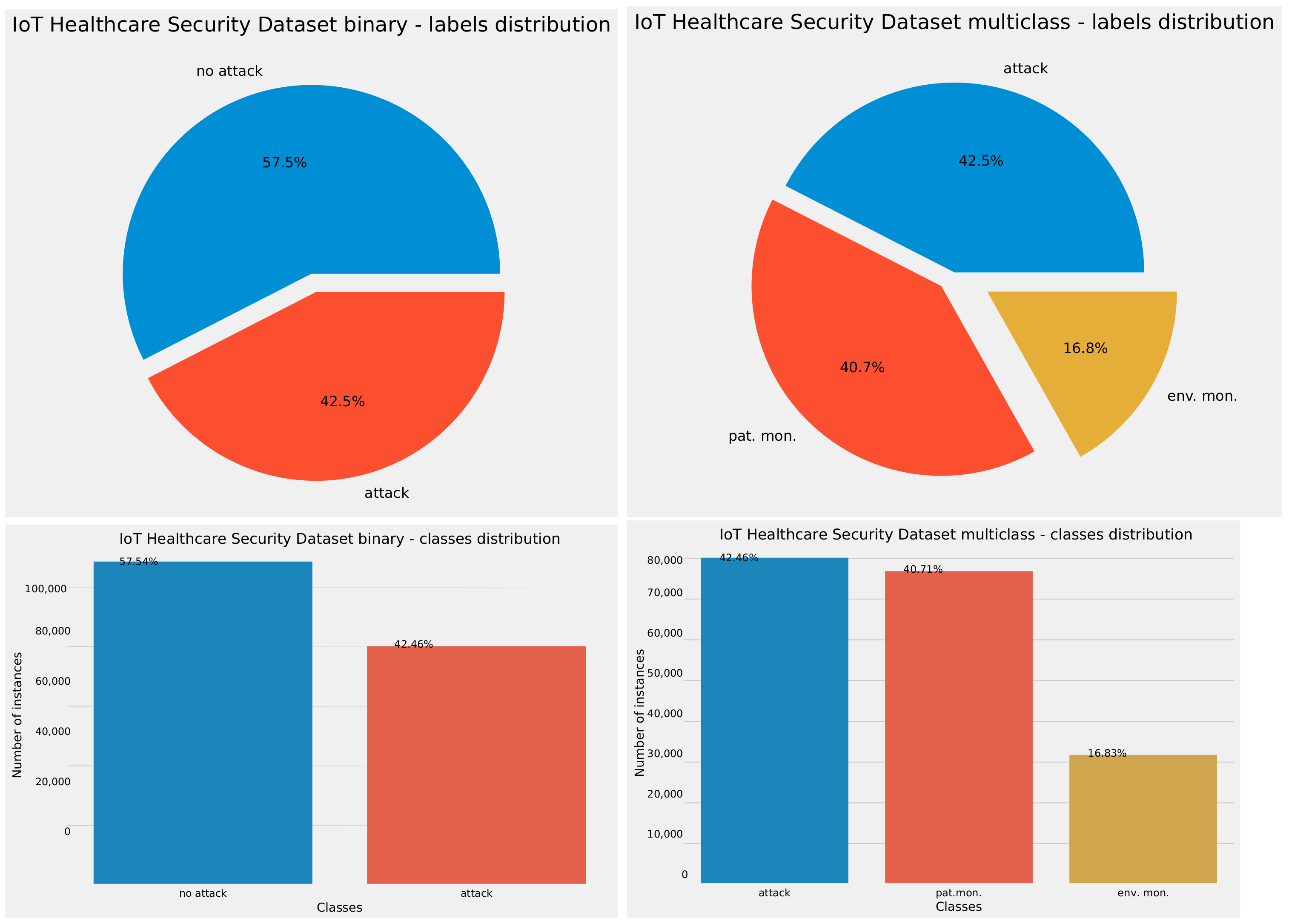
4.1. Datasets

The applied IoT healthcare security dataset [49] is a dataset generated by a tool proposed by the authors of the referenced work [17]. This research aims to recreate the experiments from the [17] to establish the basis for comparison. The dataset is publicly available at https://www.kaggle.com/datasets/faisalmalik/iot-healthcare-security-dataset (accessed on 14 July 2023).

The authors [17] applied an open-source IoT traffic generator tool IoT-Flock to create a test case for a healthcare problem. IoT-Flock is a versatile tool for creating simulation environments of normal and malicious devices assigned with IP addresses. It is noteworthy that not many such tools support the attacking capabilities of simulation. This results in traffic containing regular communication as well as attacking patterns that are paramount for better IDS and IPS design. The application supports the generation of messages that adhere to two protocols either message queuing telemetry transport (MQTT) or constrained application protocol (COAP). MQTT-generated devices require device information including the username, password, broker’s IP address, and subscribing or publishing indicators. COAP devices require the IP address of the server and the COAP command. Additionally, XML output alongside a GUI and console mode is supported by the application.

The author [49] dataset is an intensive care unit (ICU) use case that simulates an ICU with two beds each with nine sensors and one control unit labeled according to the scheme: Bedx-Control-unit, where x represents the number of each bed. This unit is responsible for time profile settings, infusion pump dosages, and the emergency alarm that shows if a patient is in need according to sensors. The dataset is created with an additional unit for environment control which sets the temperature and humidity, can detect smoke, and activate the alarm as well. Considering that the data are transmitted by sensors in certain intervals, the authors introduce two additional characteristics, the data and time profiles. Range and data type transmitted are specified by the data counterpart, while the time profile defines the intervals in which the communication between the sensors and the control unit is performed.

The process of data generation for the applied ICU dataset results in two separate networks. The first network represents a model of the described ICU unit, and the second is the network of the attacker. The targeted network consists of MQTT devices that transmit and receive data alongside an MQTT broker. These devices include the patient and environment monitors that communicate under usual circumstances. IoT-Flock creates a virtual network interface for each device on a single physical machine running Linux. The MQTT broker and COAP server were running on a different machine. The network of the invader supports the execution of various attack types on the target network. The attacker network consists of ten devices that can perform four different attack types which are the MQTT distributed denial-of-service, MQTT publish flood, brute force, and SlowITE [50]. More details on the dataset are available in the referenced work [17].

The KNN algorithm with the number of neighbors set to $K=5$ was applied for feature selection from the datasets, as the original dataset consists of 50 features in total. The best 10 features were selected for maximization of the proposed methods’ performance and this experiment confirms that the same 10 features are selected as in the referenced work [17]. The features are described in detail in [17] and include:

• frame.time_delta,
• tcp.time_delta,
• tcp.flags.ack,
• tcp.flags.push,
• tcp.flags.reset,
• mqtt.hdrflags,
• mqtt.msgtype,
• mqtt.qos,
• mqtt.retain, and
• mqtt.ver.

Due to the format of mqtt.hdrflags being hexadecimal, its values had to be converted to decimal format so that the ML method could process them.

The research that is the basis of comparison for this work [17], employs only binary classification for the problem with two types of data. The first is the regular communication without attackers and represents class 0, while the second one represents the attacking case and class 1. The performed experiments are an extension of a previous study from [17] in the form of three classes given below:

• Class 0—No attack, environment monitoring,
• Class 1—No attack, patient monitoring, and
• Class 2—Attack.

Figure 1 displays the binary and multiclass distribution of the applied datasets with pie and bar charts. The heatmap of the features is provided in Figure 2.

4.2. Experimental Setup

Optimization of XGBoost hyperparameters is performed by the proposed MFA algorithm in the case of the ICU dataset. The optimized hyperparameters along their boundaries and variable types are given in the following list:

• learning rate ($\eta$), search limits: $[0.1,0.9]$, continuous variable,
• $min\_child\_weight$, search limits: $[1,10]$, continuous variable,
• subsample, search limits: $[0.01,1]$, continuous variable,
• collsample_bytree, search limits: $[0.01,1]$, continuous variable,
• max_depth, search limits: $[3,10]$, integer variable and
• $gamma$, search limits: $[0,0.8]$, continuous variable.

The provided boundaries were obtained empirically by the trial and error method.

The proposed method is made with Python programming language alongside scipy, numpy, and pandas, standard Python libraries. The XGBoost model was provided by the sci-kit learn package.

The optimized hyperparameter number is given in the following text as l, and it is used to set the length of an array that represents a single encoded solution. The value of l is 6.

The split of the dataset was performed randomly of which 70% is for training, while the other 30% is used for the test set. The data were not normalized.

The goal of the proposed hybrid XGBoost MFA optimized method performance validation is performed by comparing with eight other optimizers including the original FA, for the same problem. The algorithms included in the comparison are the FA [34], genetic algorithm (GA) [51,52], PSO [31], artificial bee colony (ABC) algorithm [53], chimp optimization algorithm (ChOA) [54], differential evolution linear population size reduction constrained optimization with levy flights (COLSHADE) algorithm [55], and self-adapting spherical search (SASS) [56]. The tests consist of every listed algorithm performing the same test with recommended values for control parameters. All solutions have been implemented and independently tested. The same setup was established for all tested solutions with a population of 10 solutions over 10 iterations per run, over 30 runs.

4.3. Performance Metrics

The evaluation of performance was performed as in [17], due to firm comparison grounds. Accuracy, precision, recall, and F1-score are derived from confusion matrixes generated by each compared solution. It is important to emphasize that the accuracy can vary from one scenario to another as the dataset is imbalanced. Standard terminology is applied in descriptions of the measured values. True and false predictions are indicated as true positive (TP) and false positive (FP) for positive predictions, while the negative predictions are shown as false negative (FN) and true negative (TN).

The ratio of correct predictions to missed ones is accuracy [57].

$$Accuracy=\frac{TP+TN}{TP+TN+FP+FN}$$

(7)

Precision represents the ratio of correct predictions to all predicted positives.

Correct predictions and all predictions (wrong and correct) ratio is the precision [57].

$$Precision=\frac{TP}{FP+TP}$$

(8)

Correct predictions and positive cases ratio represent recall [57].

$$Recall=\frac{TP}{FN+TP}$$

(9)

Recall and precision are combined to provide F1-score [57].

$$\mathrm{F}1\text{-}\mathrm{score}=\frac{(2\times Precision\times Recall)}{(Precision+Recall)}$$

(10)

Cohen’s kappa coefficient is an agreement measure for two sets of classification while taking into account the classification randomness [58]. Odds of an event happening due to a particular factor [59] compared to the probability of the same event occurring without that factor is the odd ratio calculated by the following equation:

$$\frac{\left(\frac{TP}{FP}\right)}{\left(\frac{TN}{FN}\right)}$$

(11)

Odds of an event happening due to a particular factor [59] compared to the probability of the same event occurring without that factor is the odd ratio that represents the kappa coefficient [60] calculated by the following equation:

$$K=\frac{P_{obs}-P_{exp}}{1-P_{exp}}$$

(12)

where the observed agreements $(TP+TN)$ are represent as $P_{obs}$, while the expected agreements $[(TP+FN)\times (TP+FP)+(FP+TN)\times (FN+TN)]$ [61] are given as $P_{exp}$. The value of K is in the range $[0,1]$, while lower values indicate less agreement. Different levels of agreement are recognized: no agreement $K\le 0$, slight agreement 0.01–0.20, fair agreement 0.21–0.40, moderate agreement 0.41–0.60, substantial agreement 0.61–0.80, and near to perfect agreement 0.81–1.00 as described in [61].

5. Simulation Results, Comparative Analysis, Validation, and Interpretation

5.1. Experimental Findings and Comparative Analyssis

The

Table 1. Overall results binary classification—error minimization experiment.

	Classification Error (Objective)						Cohen’s Kappa
Method	Best	Worst	Mean	Median	Std	Var	Best	Worst	Mean	Median	Std	Var
XG-MFA	0.003003	0.003091	0.003036	0.003030	$3.24\times {10}^{-5}$	$1.05\times {10}^{-9}$	0.993852	0.993672	0.993785	0.993798	$6.63\times {10}^{-5}$	$4.40\times {10}^{-9}$
XG-FA	0.003038	0.003303	0.003153	0.003153	$7.85\times {10}^{-5}$	$6.16\times {10}^{-9}$	0.993780	0.993236	0.993545	0.993544	$1.61\times {10}^{-4}$	$2.60\times {10}^{-8}$
XG-GA	0.003038	0.003197	0.003096	0.003091	$4.82\times {10}^{-5}$	$2.32\times {10}^{-9}$	0.993781	0.993454	0.993662	0.993671	$9.87\times {10}^{-5}$	$9.75\times {10}^{-9}$
XG-PSO	0.003074	0.003215	0.003125	0.003109	$4.79\times {10}^{-5}$	$2.30\times {10}^{-9}$	0.993708	0.993418	0.993604	0.993635	$9.82\times {10}^{-5}$	$9.64\times {10}^{-9}$
XG-ABC	0.003109	0.003374	0.003213	0.003171	$8.49\times {10}^{-5}$	$7.21\times {10}^{-9}$	0.993636	0.993092	0.993422	0.993508	$1.74\times {10}^{-4}$	$3.03\times {10}^{-8}$
XG-SSA	0.003038	0.003233	0.003138	0.003144	$5.99\times {10}^{-5}$	$3.58\times {10}^{-9}$	0.993781	0.993381	0.993576	0.993563	$1.23\times {10}^{-4}$	$1.52\times {10}^{-8}$
XG-ChOA	0.003038	0.003180	0.003105	0.003100	$4.21\times {10}^{-5}$	$1.77\times {10}^{-9}$	0.993780	0.993490	0.993644	0.993653	$8.65\times {10}^{-5}$	$7.49\times {10}^{-9}$
XG-COLSHADE	0.003021	0.003215	0.003102	0.003091	$5.85\times {10}^{-5}$	$3.43\times {10}^{-9}$	0.993817	0.993419	0.993649	0.993671	$1.19\times {10}^{-4}$	$1.44\times {10}^{-8}$
XG-SASS	0.003021	0.003162	0.003105	0.003118	$4.65\times {10}^{-5}$	$2.16\times {10}^{-9}$	0.993815	0.993526	0.993644	0.993616	$9.53\times {10}^{-5}$	$9.09\times {10}^{-9}$

provides overall results for binary classification for error minimization experiment. The results of precision, recall, and F1-score are provided in

Table 2. Detailed results per classes for best performing binary classification models—error minimization experiment.

Method	Metric	0	1	Macro Avg	Weighted Avg
XG-MFA	precision	0.996567	0.997582	0.997074	0.996998
	recall	0.998219	0.995341	0.996780	0.996997
	f1-score	0.997392	0.996460	0.996926	0.996996
XG-FA	precision	0.996628	0.997416	0.997022	0.996962
	recall	0.998096	0.995424	0.996760	0.996962
	f1-score	0.997362	0.996419	0.996890	0.996961
XG-GA	precision	0.996780	0.997208	0.996994	0.996962
	recall	0.997943	0.995632	0.996787	0.996962
	f1-score	0.997361	0.996420	0.996890	0.996961
XG-PSO	precision	0.996536	0.997457	0.996997	0.996927
	recall	0.998127	0.995299	0.996713	0.996926
	f1-score	0.997331	0.996377	0.996854	0.996927
XG-ABC	precision	0.996506	0.997415	0.996960	0.996892
	recall	0.998096	0.995258	0.996677	0.996891
	f1-score	0.997300	0.996335	0.996818	0.996891
XG-SSA	precision	0.996841	0.997125	0.996983	0.996962
	recall	0.997882	0.995715	0.996798	0.996962
	f1-score	0.997361	0.996420	0.996890	0.996961
XG-ChOA	precision	0.996293	0.997872	0.997083	0.996964
	recall	0.998434	0.994966	0.996700	0.996962
	f1-score	0.997362	0.996417	0.996890	0.996961
XG-COLSHADE	precision	0.996719	0.997333	0.997026	0.996980
	recall	0.998035	0.995549	0.996792	0.996979
	f1-score	0.997377	0.996440	0.996908	0.996979
XG-SASS	precision	0.996020	0.998288	0.997154	0.996983
	recall	0.998741	0.994592	0.996667	0.996979
	f1-score	0.997379	0.996437	0.996908	0.996979
	support	32,571	24,038	56,609	56,609

. XG-MFA obtains the highest F1-scores for both classes, macro average, and the weighted average for all other metrics besides the F1-score unlike the previously stated. XG-GA had the best 0 class precision, XG-SSA the best recall for class 0 and macro average, XG-ChOA the best precision for macro average, while the XG-SASS provides the best class 1 precision along the best class 0 recall. Confirming the proposed method’s performance on the binary classification error minimization optimization the XG-MFA obtained the highest results in accuracy terms. The best obtained results are indicating with bold font.

The settings of hyperparameters for the binary classification for error minimization are provided in

Table 3. Best obtained models’ hyper-parameters binary classification—error minimization experiment.

Method	Learning Rate	Min Child Weight	Subsample	Colsample by Tree	Max Depth	Gamma
XG-MFA	0.826864	1.781749	0.801824	0.663691	10	0.120070
XG-FA	0.900000	1.128921	0.793675	0.871647	10	0.800000
XG-GA	0.788252	1.000000	1.000000	1.000000	10	0.000000
XG-PSO	0.602643	1.000000	0.680449	1.000000	10	0.800000
XG-ABC	0.900000	1.000000	0.673743	1.000000	7	0.323973
XG-SSA	0.748588	1.216229	1.000000	1.000000	10	0.023409
XG-ChOA	0.774825	1.000000	1.000000	1.000000	10	0.567155
XG-COLSHADE	0.900000	2.324410	0.826696	0.781224	10	0.259289
XG-SASS	0.900000	1.000000	0.980985	0.632832	8	0.149104

.

The Figure 3 displays multiple plots for the binary minimization experiment. The objective convergence and box plot are provided with a swarm plot displaying diversity, along the precision recall curve, receiver operating characteristics curve, and the confusion matrix.

Secondly, the problem of binary classification for Cohen’s kappa coefficient maximization problem is tested due to the imbalanced dataset that is used.

Table 4. Overall results binary classification—Cohen’s kappa coefficient maximization experiment.

	Cohen’s Kappa (Objective)						Classification Error
Method	Best	Worst	Mean	Median	Std	Var	Best	Worst	Mean	Median	Std	Var
XG-MFA	0.993817	0.993707	0.993780	0.993780	$3.64\times {10}^{-5}$	$1.33\times {10}^{-9}$	0.003021	0.003074	0.003038	0.003038	$1.77\times {10}^{-5}$	$3.12\times {10}^{-10}$
XG-FA	0.993746	0.993345	0.993577	0.993581	$1.36\times {10}^{-4}$	$1.84\times {10}^{-8}$	0.003056	0.003250	0.003138	0.003136	$6.61\times {10}^{-5}$	$4.36\times {10}^{-9}$
XG-GA	0.993707	0.993454	0.993621	0.993635	$7.47\times {10}^{-5}$	$5.57\times {10}^{-9}$	0.003074	0.003197	0.003116	0.003109	$3.64\times {10}^{-5}$	$1.32\times {10}^{-9}$
XG-PSO	0.993744	0.993526	0.993644	0.993689	$8.44\times {10}^{-5}$	$7.12\times {10}^{-9}$	0.003056	0.003162	0.003105	0.003083	$4.12\times {10}^{-5}$	$1.70\times {10}^{-9}$
XG-ABC	0.993707	0.993200	0.993413	0.993381	$1.72\times {10}^{-4}$	$2.97\times {10}^{-8}$	0.003074	0.003321	0.003217	0.003233	$8.40\times {10}^{-5}$	$7.06\times {10}^{-9}$
XG-SSA	0.993745	0.993562	0.993690	0.993707	$5.46\times {10}^{-5}$	$2.99\times {10}^{-9}$	0.003056	0.003144	0.003083	0.003074	$2.65\times {10}^{-5}$	$7.02\times {10}^{-10}$
XG-ChOA	0.993744	0.993164	0.993585	0.993617	$1.68\times {10}^{-4}$	$2.86\times {10}^{-8}$	0.003056	0.003339	0.003133	0.003118	$8.24\times {10}^{-5}$	$6.78\times {10}^{-9}$
XG-COLSHADE	0.993780	0.993164	0.993545	0.993581	$1.91\times {10}^{-4}$	$3.67\times {10}^{-8}$	0.003038	0.003339	0.003153	0.003136	$9.35\times {10}^{-5}$	$8.74\times {10}^{-9}$
XG-SASS	0.993781	0.993345	0.993604	0.993617	$1.30\times {10}^{-4}$	$1.69\times {10}^{-8}$	0.003038	0.003250	0.003125	0.003118	$6.33\times {10}^{-5}$	$4.01\times {10}^{-9}$

provides general metrics like Table 1, in which the XG-MFA once again dominates only this time the shortcomings are recorded as the XG-ABC provides the best results for class 0 best, worst, mean, median, and standard deviation. The rest of the results are in favor of XG-MFA.

Furthermore, a similar performance is recorded with kappa maximization metrics as in Table 2, where the proposed method obtains the best results except for precision and recall for class 0, class 1, and macro average. The details are provided in

Table 5. Detailed results per classes for best performing binary classification models—Cohen’s kappa coefficient maximization experiment.

Method	Metric	0	1	Macro Avg	Weighted Avg
XG-MFA	precision	0.996811	0.997208	0.997010	0.996980
	recall	0.997943	0.995674	0.996808	0.996979
	f1-score	0.997376	0.996440	0.996908	0.996979
XG-FA	precision	0.996780	0.997167	0.996973	0.996944
	recall	0.997912	0.995632	0.996772	0.996944
	f1-score	0.997346	0.996399	0.996872	0.996944
XG-GA	precision	0.996080	0.998080	0.997080	0.996929
	recall	0.998588	0.994675	0.996631	0.996926
	f1-score	0.997332	0.996376	0.996853	0.996926
XG-PSO	precision	0.996475	0.997581	0.997028	0.996945
	recall	0.998219	0.995216	0.996718	0.996944
	f1-score	0.997347	0.996397	0.996872	0.996943
XG-ABC	precision	0.996262	0.997830	0.997046	0.996928
	recall	0.998403	0.994925	0.996664	0.996926
	f1-score	0.997332	0.996375	0.996854	0.996926
XG-SSA	precision	0.996780	0.997167	0.996973	0.996944
	recall	0.997912	0.995632	0.996772	0.996944
	f1-score	0.997346	0.996399	0.996872	0.996944
XG-ChOA	precision	0.996597	0.997415	0.997006	0.996945
	recall	0.998096	0.995382	0.996739	0.996944
	f1-score	0.997346	0.996398	0.996872	0.996944
XG-COLSHADE	precision	0.996323	0.997831	0.997077	0.996963
	recall	0.998403	0.995008	0.996706	0.996962
	f1-score	0.997362	0.996417	0.996890	0.996961
XG-SASS	precision	0.996719	0.997291	0.997005	0.996962
	recall	0.998004	0.995549	0.996777	0.996962
	f1-score	0.997361	0.996419	0.996890	0.996961
	support	32,571	24,038	56,609	56,609

.

The settings of hyperparameters for the binary classification for kappa maximization are provided in

Table 6. Best obtained models’ hyper-parameters binary classification—Cohen’s kappa coefficient maximization experiment.

Method	Learning Rate	Min Child Weight	Subsample	Colsample by Tree	Max Depth	Gamma
XG-MFA	0.900000	1.000000	0.993956	0.790192	10	0.166214
XG-FA	0.900000	1.000000	1.000000	1.000000	10	0.000000
XG-GA	0.900000	1.929015	1.000000	0.821090	10	0.800000
XG-PSO	0.900000	1.000000	0.979482	1.000000	10	0.061248
XG-ABC	0.625776	1.000000	0.627028	0.970949	10	0.371569
XG-SSA	0.900000	1.000000	1.000000	1.000000	10	0.000000
XG-ChOA	0.876269	1.576144	0.660126	0.766469	10	0.800000
XG-COLSHADE	0.874638	1.584114	1.000000	1.000000	10	0.000000
XG-SASS	0.900000	1.298750	0.885388	1.000000	10	0.358750

.

The plots for the Cohen’s kappa experiment are provided in the Figure 4 in the same manner as for the error minimization experiments as in Figure 3.

Table 7. Overall results multiclass classification—error minimization experiment.

	Classification Error (Objective)						Cohen’s Kappa
Method	Best	Worst	Mean	Median	Std	Var	Best	Worst	Mean	Median	Std	Var
XG-MFA	0.008232	0.008462	0.008322	0.008320	$9.30\times {10}^{-5}$	$8.66\times {10}^{-9}$	0.986843	0.986475	0.986699	$0.96704$	$1.49\times {10}^{-4}$	$2.22\times {10}^{-8}$
XG-FA	0.008320	0.008797	0.008473	0.008409	$1.58\times {10}^{-4}$	$2.53\times {10}^{-8}$	0.986704	0.985939	0.986458	0.986560	$2.54\times {10}^{-4}$	$6.46\times {10}^{-8}$
XG-GA	0.008356	0.008603	0.008446	0.008435	$7.97\times {10}^{-5}$	$6.35\times {10}^{-9}$	0.986645	0.986251	0.986499	0.986516	$1.27\times {10}^{-4}$	$1.62\times {10}^{-8}$
XG-PSO	0.008409	0.008727	0.008499	0.008444	$9.73\times {10}^{-5}$	$9.47\times {10}^{-9}$	0.986559	0.986052	0.986415	0.986502	$1.55\times {10}^{-4}$	$2.41\times {10}^{-8}$
XG-ABC	0.008426	0.008992	0.008687	0.008691	$1.71\times {10}^{-4}$	$2.93\times {10}^{-8}$	0.986532	0.985628	0.986114	0.986107	$2.74\times {10}^{-4}$	$7.52\times {10}^{-8}$
XG-SSA	0.008356	0.008550	0.008446	0.008426	$7.77\times {10}^{-5}$	$6.04\times {10}^{-9}$	0.986643	0.986334	0.986500	0.986532	$1.25\times {10}^{-4}$	$1.56\times {10}^{-8}$
XG-ChOA	0.008373	0.008568	0.008464	0.008462	$7.20\times {10}^{-5}$	$5.18\times {10}^{-9}$	0.986615	0.986305	0.986471	0.986474	$1.15\times {10}^{-4}$	$1.33\times {10}^{-8}$
XG-COLSHADE	0.008303	0.008479	0.008375	0.008364	$5.55\times {10}^{-5}$	$3.08\times {10}^{-9}$	0.986729	0.986445	0.986612	0.986629	$8.89\times {10}^{-5}$	$7.91\times {10}^{-9}$
XG-SASS	0.008391	0.008850	0.008515	0.008506	$1.37\times {10}^{-4}$	$1.90\times {10}^{-8}$	0.986588	0.985855	0.986391	0.986405	$2.20\times {10}^{-4}$	$4.84\times {10}^{-8}$

shows the multiclassification error of the metaheuristics methods. XG-MFA performs the best on all performance indicators except for standard deviation and variance. XG-COLSHADE shows the least variation in its performance, as indicated by having the lowest values for both standard deviation and variance. This could be a significant factor when looking for models with consistent results. XG-ABC seems to perform the worst.

Table 8. Detailed results per classes for best performing multiclass classification models—error minimization simulation.

Method	Metric	0	1	2	Macro Avg	Weighted Avg
XG-MFA	precision	0.976150	0.992045	0.997705	0.988633	0.991773
	recall	0.975126	0.995747	0.994550	0.988474	0.991768
	f1-score	0.975638	0.993892	0.996125	0.988552	0.991768
XG-FA	precision	0.974445	0.992598	0.997663	0.988235	0.991693
	recall	0.976490	0.995140	0.994384	0.988671	0.991680
	f1-score	0.975467	0.993867	0.996021	0.988451	0.991686
XG-GA	precision	0.975531	0.992129	0.997580	0.988413	0.991650
	recall	0.974916	0.995617	0.994467	0.988333	0.991644
	f1-score	0.975223	0.993870	0.996021	0.988371	0.991645
XG-PSO	precision	0.975925	0.992340	0.997082	0.988449	0.991591
	recall	0.974286	0.995140	0.995050	0.988158	0.991591
	f1-score	0.975105	0.993738	0.996065	0.988303	0.991590
XG-ABC	precision	0.975525	0.991957	0.997580	0.988354	0.991579
	recall	0.974706	0.995487	0.994509	0.988234	0.991574
	f1-score	0.975115	0.993719	0.996042	0.988292	0.991574
XG-SSA	precision	0.976835	0.991917	0.997247	0.988666	0.991642
	recall	0.973657	0.995834	0.994758	0.988083	0.991644
	f1-score	0.975243	0.993871	0.996001	0.988372	0.991640
XG-ChOA	precision	0.976331	0.992086	0.997248	0.988555	0.991626
	recall	0.974076	0.995573	0.994800	0.988150	0.991627
	f1-score	0.975202	0.993827	0.996022	0.988350	0.991624
XG-COLSHADE	precision	0.976441	0.992257	0.997206	0.988635	0.991697
	recall	0.974391	0.995530	0.994883	0.988268	0.991697
	f1-score	0.975415	0.993891	0.996043	0.988450	0.991695
XG-SASS	precision	0.976028	0.992257	0.997164	0.988483	0.991609
	recall	0.974286	0.995443	0.994600	0.988177	0.991609
	f1-score	0.975156	0.993847	0.995981	0.988328	0.991607
	support	9528	23,043	24,038	56,609	56,609

shows the performance evaluation results using precision, recall, and f1-score metrics for each class (0, 1, 2), as well as the macro average and weighted average across classes. The support row at the bottom indicates the number of instances for each class in the dataset. XG-MFA performs the best in terms of overall precision, recall, and f1-score (weighted average). It also performs best for the precision and f1-score of class 2. XG-FA has the highest recall for class 0 and the highest precision for class 1. However, it does not lead to macro averages or weighted averages. XG-PSO has the highest recall for class 2, indicating it is the best at correctly identifying positive instances of class 2. XG-SSA has the highest precision for class 0 and achieves the highest macro average for precision, which means it performs well at correctly predicting the positive class across the different classes without taking class imbalance into account. The recall of class 1 is the highest for XG-SSA, suggesting that this method is particularly effective in identifying instances of class 1. In general, while some methods may excel in certain metrics, the XG-MFA method appears to be the most balanced, performing very well across all metrics and classes. This suggests that XG-MFA may be the best choice for applications where all classes and metrics are equally important. Also, note that class distribution is imbalanced (Class 0: 9528, Class 1: 23,043, Class 2: 24,038). This might affect the performance of these models, as they could be biased toward the majority classes (classes 1 and 2). The weighted average metric, which takes this imbalance into account, can provide a better overall evaluation of model performance than the macro average.

The combined previous analysis of error metrics and precision, recall, and f1-score reinforces the conclusion that XG-MFA generally performs the best among these algorithms.

Hyperparameter settings are provided for the multiclass classification for error minimization in the

Table 9. Best obtained models’ hyper-parameters multiclass classification—error minimization experiment.

Method	Learning Rate	Min Child Weight	Subsample	Colsample by Tree	Max Depth	Gamma
XG-MFA	0.558224	1.390646	1.000000	0.754489	10	0.800000
XG-FA	0.900000	2.356392	1.000000	1.000000	7	0.800000
XG-GA	0.532608	1.671261	1.000000	1.000000	9	0.595526
XG-PSO	0.900000	1.209953	1.000000	0.965372	10	0.162178
XG-ABC	0.516726	1.000000	0.796465	0.842297	10	0.518501
XG-SSA	0.643381	1.000000	1.000000	0.864255	10	0.087284
XG-ChOA	0.650355	1.000000	1.000000	0.800611	10	0.000000
XG-COLSHADE	0.578265	1.981063	1.000000	0.761847	10	0.010795
XG-SASS	0.900000	2.028573	1.000000	1.000000	10	0.800000

.

Table 10. Overall results multiclass classification—Cohen’s kappa coefficient maximization experiment.

	Cohen’s kappa (Objective)						Classification Error
Method	Best	Worst	Mean	Median	Std	Var	Best	Worst	Mean	Median	Std	Var
XG-MFA	0.986785	0.986417	0.986670	0.986670	$1.25\times {10}^{-4}$	$1.56\times {10}^{-8}$	0.008267	0.008497	0.008339	0.008338	$7.80\times {10}^{-5}$	$6.11\times {10}^{-9}$
XG-FA	0.986646	0.986416	0.986585	0.986589	$6.76\times {10}^{-5}$	$4.58\times {10}^{-9}$	0.008356	0.008497	0.008393	0.008391	$4.18\times {10}^{-5}$	$1.75\times {10}^{-9}$
XG-GA	0.986646	0.985630	0.986348	0.986446	$2.93\times {10}^{-4}$	$8.62\times {10}^{-8}$	0.008356	0.008992	0.008541	0.008479	$1.84\times {10}^{-4}$	$3.39\times {10}^{-8}$
XG-PSO	0.986532	0.986136	0.986369	0.986405	$1.55\times {10}^{-4}$	$2.41\times {10}^{-8}$	0.008426	0.008674	0.008528	0.008506	$9.71\times {10}^{-5}$	$9.42\times {10}^{-9}$
XG-ABC	0.986502	0.986052	0.986224	0.986207	$1.54\times {10}^{-4}$	$2.38\times {10}^{-8}$	0.008444	0.008727	0.008618	0.008629	$9.65\times {10}^{-5}$	$9.32\times {10}^{-9}$
XG-SSA	0.986644	0.986078	0.986418	0.986460	$1.65\times {10}^{-4}$	$2.75\times {10}^{-8}$	0.008356	0.008709	0.008497	0.008470	$1.04\times {10}^{-4}$	$1.08\times {10}^{-8}$
XG-ChOA	0.986589	0.986303	0.986457	0.986460	$8.53\times {10}^{-5}$	$7.27\times {10}^{-9}$	0.008391	0.008568	0.008473	0.008470	$5.29\times {10}^{-5}$	$2.80\times {10}^{-9}$
XG-COLSHADE	0.986645	0.986277	0.986511	0.986546	$1.18\times {10}^{-4}$	$1.41\times {10}^{-8}$	0.008356	0.008585	0.008439	0.008417	$7.38\times {10}^{-5}$	$5.44\times {10}^{-9}$
XG-SASS	0.986702	0.986563	0.986603	0.986589	$3.96\times {10}^{-5}$	$1.57\times {10}^{-9}$	0.008320	0.008409	0.008382	0.008391	$2.50\times {10}^{-5}$	$6.24\times {10}^{-10}$

presents the results of Cohen’s kappa coefficient for different XGBoost-based metaheuristic methods. Cohen’s kappa statistic is a measure of inter-rater reliability. It is used to measure the agreement between two raters who each classify items into mutually exclusive categories. In this case, it is being used to evaluate the performance of these machine-learning models. From this table, it can be seen that XG-MFA has the highest mean and median kappa coefficient, indicating that on average, this method tends to outperform the others in terms of inter-rater reliability. It also has the highest best value, suggesting that in the best case, this method has the highest agreement between predicted and actual labels. On the other hand, XG-SASS has the lowest standard deviation and variance for the kappa coefficient, indicating that the performance of this method is the most consistent. The performance of this method varies the least from the mean performance.

The Figure 5 represents the same plots as Figure 3 and Figure 4 for the multiclass experiment of error minimization, while the Figure 6 does so for the Cohen’s kappa multiclass maximization experiment.

Table 11. Detailed results per classes for best performing multiclass classification models—Cohen’s kappa coefficient maximization simulation.

Method	Metric	0	1	2	Macro Avg	Weighted Avg
XG-MFA	precision	0.976446	0.991833	0.997704	0.988661	0.991736
	recall	0.974601	0.996094	0.994342	0.988346	0.991733
	f1-score	0.975523	0.993959	0.996020	0.988501	0.991731
XG-FA	precision	0.975333	0.992213	0.997580	0.988375	0.991651
	recall	0.975231	0.995357	0.994592	0.988393	0.991644
	f1-score	0.975282	0.993782	0.996084	0.988383	0.991646
XG-GA	precision	0.975142	0.992085	0.997788	0.988338	0.991655
	recall	0.975756	0.995400	0.994342	0.988499	0.991644
	f1-score	0.975449	0.993740	0.996062	0.988417	0.991647
XG-PSO	precision	0.975223	0.992467	0.997206	0.988300	0.991578
	recall	0.974916	0.995226	0.994675	0.988272	0.991574
	f1-score	0.975070	0.993846	0.995939	0.988285	0.991574
XG-ABC	precision	0.976521	0.991830	0.997247	0.988533	0.991554
	recall	0.973447	0.995704	0.994758	0.987970	0.991556
	f1-score	0.974981	0.993763	0.996001	0.988247	0.991552
XG-SSA	precision	0.976333	0.992086	0.997289	0.988570	0.991644
	recall	0.974181	0.995617	0.994758	0.988186	0.991644
	f1-score	0.975256	0.993849	0.996022	0.988376	0.991642
XG-ChOA	precision	0.975126	0.992086	0.997704	0.988305	0.991617
	recall	0.975126	0.995573	0.994342	0.988347	0.991609
	f1-score	0.975126	0.993827	0.996020	0.988324	0.991611
XG-COLSHADE	precision	0.975535	0.992086	0.997621	0.988414	0.991651
	recall	0.975126	0.995573	0.994425	0.988375	0.991644
	f1-score	0.975331	0.993827	0.996021	0.988393	0.991645
XG-SASS	precision	0.975436	0.992173	0.997663	0.988424	0.991687
	recall	0.975231	0.995704	0.994342	0.988426	0.991680
	f1-score	0.975333	0.993935	0.996000	0.988423	0.991681
	support	9528	23,043	24,038	56,609	56,609

presents a breakdown of precision, recall, and f1-score metrics for different XGBoost-based metaheuristic methods for multi-classification tasks. These metrics are calculated for each of the three classes (0, 1, 2) as well as their macro and weighted averages. The XG-MFA method has the highest macro average and weighted average in precision, recall, and f1-score, suggesting it tends to have the best overall performance among the methods. It is also interesting to see the performance of the models on individual classes. For instance, the XG-GA method achieves the best recall for class 0, XG-MFA for class 1, and XG-PSO for class 2.

Table 12. Best obtained models’ hyper-parameters multiclass classification—Cohen’s kappa coefficient maximization experiment.

Method	Learning Rate	Min Child Weight	Subsample	Colsample by Tree	Max Depth	Gamma
XG-MFA	0.780152	1.000000	1.000000	1.000000	9	0.517589
XG-FA	0.900000	1.265482	1.000000	0.983060	9	0.222017
XG-GA	0.506328	1.000000	0.816145	0.945690	10	0.800000
XG-PSO	0.837106	1.000000	1.000000	1.000000	10	0.559077
XG-ABC	0.566515	2.084170	0.989990	1.000000	10	0.569104
XG-SSA	0.897294	1.103403	1.000000	1.000000	10	0.612487
XG-ChOA	0.900000	1.000000	1.000000	1.000000	9	0.800000
XG-COLSHADE	0.465601	3.091252	1.000000	1.000000	9	0.800000
XG-SASS	0.900000	1.107956	1.000000	1.000000	9	0.800000

summarizes metaheuristics hyperparameters on which evaluation of Multiclassification Cohen’s kappa coefficient was performed.

5.2. Statistical Validation

In order to further evaluate the experimental outcomes and establish their statistical significance, the highest scores obtained from 30 independent runs of each algorithm under consideration were collected and analyzed as a series of data. The initial step involves determining the appropriate type of statistical tests, whether they should be parametric or non-parametric. Initially, the suitability of parametric tests is assessed by examining the independence, normality, and homoscedasticity of the variance in the data [62]. The independence criterion is satisfied as every individual run of the metaheuristics begins with the generation of a random set of solutions.

The normality assumption was assessed through the use of the Shapiro–Wilk test, with individual problem analysis [63] for all four experiments that were conducted as part of research: binary classification (error and Cohen’s kappa as objectives), and multiclass classification (error and Cohen’s kappa as objectives). The Shapiro–Wilk test was independently applied to each of the algorithms under consideration in all four regarded scenarios, yielding p-values for each. In all instances, the resulting p-values were found to be smaller than 0.05, indicating that the null hypothesis (H0) can be rejected. Therefore, it can be concluded that the observed results are not originating from the normal distribution in all four scenarios. The Shapiro–Wilk test scores for all four scenarios are provided in

Table 13. Shapiro Wilk normality tests.

Problem	XG-MFA	XG-FA	XG-GA	XG-PSO	XG-ABC	XG-SSA	XG-ChOA	XG-COLSHADE	XG-SASS
Binary Error	0.048	0.041	0.045	0.038	0.036	0.032	0.043	0.026	0.019
Binary Kappa	0.042	0.042	0.040	0.036	0.039	0.033	0.045	0.035	0.026
Multiclass Error	0.021	0.030	0.042	0.031	0.043	0.025	0.019	0.020	0.023
Multiclass Kappa	0.035	0.038	0.021	0.040	0.035	0.029	0.042	0.027	0.030

.

Since the normality condition was not fulfilled, it is not safe to apply the parametric tests. Consequently, it was proceeded by applying the non-parametric Wilcoxon signed-rank test [64] utilizing the identical data series containing the best values obtained in each run.

The suggested MFA was utilized as the control method, and Wilcoxon signed-rank test has been conducted over the above-mentioned data series. The calculated p-values were in all cases lower than 0.05, for all four observed scenarios. These results clearly suggest that the introduced MFA method performed statistically significantly better in comparison to all contenders for both significance thresholds $alpha=0.1$ and $alpha=0.05$. The outcomes of Wilcoxon singed-rank test have been provided within

Table 14. Wilcoxon signed-rank test scores representing p-values for all four scenarios (XG-MFA vs. others).

Problem/p-Values	XG-FA	XG-GA	XG-PSO	XG-ABC	XG-SSA	XG-ChOA	XG-COLSHADE	XG-SASS
Binary Error	0.016	0.037	0.028	0.008	0.025	0.031	0.034	0.031
Binary Kappa	0.025	0.036	0.026	0.027	0.031	0.029	0.040	0.039
Multiclass Error	0.034	0.035	0.030	0.019	0.035	0.035	0.041	0.027
Multiclass Kappa	0.040	0.026	0.028	0.024	0.042	0.036	0.038	0.033

.

5.3. Best Models Results Interpretation

SHAP analysis has been recognized as a method for bringing transparency to model performance. Additionally, two different types of SHAP analysis are provided for the performed experiments. First, XGBoost feature importance is established. The importance is determined by considering the weights of the evaluated nodes, and in the case of higher observation dependence on the subject node, the importance is considered higher. The importance is calculated on a single decision tree and averaged over the rest of the trees. Determined feature importance for the best-attained models in both experiments are shown in Figure 7.

Outcomes demonstrated in Figure 7a suggest that based on importance determined by XGBoost, tcp.time_delta plays a high role in determining outcomes in binary classification, followed by the frame.time_detlta, mqtt.hdrflags and mqtt.msgtype features. While additional features are considered they demonstrated lower importance. Similar outcomes are demonstrated for multi-class classification in Figure 7b, with tcp.time_delta showing high importance in determining outcomes. However, relative to the importance of binary classification, the impact is somewhat lower. This feature is similarly followed by frame.time_delta and mqtt.hdrflags features, which now show a higher impact relative to binary classification.

Feature impact is calculated using SHAP similarly through the approximation approach. The process is performed with a given number of samples and the feature importance is calculated locally, on the current set. Analysis has been conducted for both binary and multi-class experiments, and their outcomes are demonstrated in Figure 8.

Feature impact outcomes for binary classification shown in Figure 8a suggest that tcp.time_delta contributes roughly equally to both classes, similarly to frame.time_delta the second highest rated feature. However, outcomes for the mqtt.dfrflages suggest that it plays a more signification role in class 1 classification. The remaining features show a high impact on class 0 decisions. Analysis outcomes for multi-class experiments shown in Figure 8b mirror previous findings, with tcp.time_delta, mqtt.hdrflags, frame.time_delta and tcp.flags.push showing the highest rate of impact. However, class-wise impacts are interesting, indicating that class 1 decisions are mostly impacted by the first two features.

Lastly, nSHAP analysis was performed for the order of 2, 10, and the Shapley–Taylor analysis. This allows us to determine to what extent features, including classification, count toward a certain outcome away from a certain classification being made. In total, three analyses were conducted that utilized nSHAP. Determined n-Shapley values up to the 10th order are shown in Figure 9.

The outcomes of the nSHAP analysis help us observe that interactions between features exist in the higher order for many of the features both for binary and multi-class classification. Additionally, many of the higher-order interactions demonstrate interesting outcomes, often contributing differently to what is experienced for the main contributions.

Table 15. IoT-Flock generated healthcare dataset commonly used machine learning classifier performance for malicious and normal traffic prediction.

ML Classifier	Precision	Recall	Accuracy	F1-Score
NB	79.6712	99.7052	52.1821	68.5093
KNN	99.6501	99.6865	99.4872	99.5868
RF	99.7069	99.7954	99.5121	99.6534
AB	99.5547	99.4457	99.5037	99.4748
LogR	95.2879	90.3515	99.5036	94.7071
DT	99.6945	99.7992	99.4788	99.6389
XG-MFA	99.6998	99.6997	99.6997	99.6996

displays the proposed model’s performance compared to the most used machine-learning techniques for similar classification problems. The performance was evaluated by the error minimization problem. The results confirm the performance of the novel solution as it obtains the highest scores for all metrics, except recall where the decision tree obtained the best score.

The attained Shapley–Taylor interaction index outcomes can be observed in Figure 10.

Finally, faithful Shapley interaction index can be seen in Figure 11.

6. Conclusions

The exploration of machine learning algorithms, particularly those optimized by the modified firefly algorithm, has offered a profound perspective on addressing the security challenges associated with the integration of IoT in Healthcare 4.0.

The models developed in this study have demonstrated impressive performance in detecting security issues within IoT devices used in healthcare, emphasizing the efficacy and potential of machine learning coupled with the modified firefly metaheuristics. Notably, XG-MFA emerged as a highly accurate model, exhibiting an accuracy of 0.991733 in multi-classification tasks, underlining its proficiency in addressing complex, real-world security detection challenges.

Further, the application of SHAP enabled a deeper understanding of the factors contributing to security issues in IoT devices. By identifying these key influencers, we can enhance our prevention strategies and design more robust and secure systems, thereby promoting the sustainability of IoT systems in healthcare.

Our results highlight the power and importance of using advanced, optimized machine learning techniques in cybersecurity within the healthcare sector. Nevertheless, despite the promising results achieved, this area still has vast untapped potential. We encourage future work to further explore and enhance the use of machine learning algorithms in ensuring the security of IoT devices in healthcare, especially in light of the rapid development and integration of IoT systems in everyday life.

In conclusion, while challenges persist in the integration of IoT in healthcare, this study proves that strategic use of machine learning algorithms, like the ones optimized by the modified firefly algorithm, can significantly mitigate these issues. This paves the way for sustainable, secure, and more effective healthcare supported by the Internet of Things.

References

- Wehde, M. Healthcare 4.0. IEEE Eng. Manag. Rev. 2019, 47, 24–28. [Google Scholar] [CrossRef]
- Hathaliya, J.J.; Tanwar, S. An exhaustive survey on security and privacy issues in Healthcare 4.0. Comput. Commun. 2020, 153, 311–335. [Google Scholar] [CrossRef]
- Hathaliya, J.J.; Tanwar, S.; Tyagi, S.; Kumar, N. Securing electronics healthcare records in healthcare 4.0: A biometric-based approach. Comput. Electr. Eng. 2019, 76, 398–410. [Google Scholar] [CrossRef]
- Amjad, A.; Kordel, P.; Fernandes, G. A Review on Innovation in Healthcare Sector (Telehealth) through Artificial Intelligence. Sustainability 2023, 15, 6655. [Google Scholar] [CrossRef]
- Krishnamoorthy, S.; Dua, A.; Gupta, S. Role of emerging technologies in future IoT-driven Healthcare 4.0 technologies: A survey, current challenges and future directions. J. Ambient. Intell. Humaniz. Comput. 2023, 14, 361–407. [Google Scholar] [CrossRef]
- Ali, M.H.; Jaber, M.M.; Abd, S.K.; Rehman, A.; Awan, M.J.; Damaševičius, R.; Bahaj, S.A. Threat Analysis and Distributed Denial of Service (DDoS) Attack Recognition in the Internet of Things (IoT). Electronics 2022, 11, 494. [Google Scholar] [CrossRef]
- Padmashree, A.; Krishnamoorthi, M. Decision Tree with Pearson Correlation-based Recursive Feature Elimination Model for Attack Detection in IoT Environment. Inf. Technol. Control 2022, 51, 771–785. [Google Scholar] [CrossRef]
- Rana, S.K.; Rana, S.K.; Nisar, K.; Ag Ibrahim, A.A.; Rana, A.K.; Goyal, N.; Chawla, P. Blockchain technology and Artificial Intelligence based decentralized access control model to enable secure interoperability for healthcare. Sustainability 2022, 14, 9471. [Google Scholar] [CrossRef]
- Guezzaz, A.; Azrour, M.; Benkirane, S.; Mohy-Eddine, M.; Attou, H.; Douiba, M. A lightweight hybrid intrusion detection framework using machine learning for edge-based IIoT security. Int. Arab. J. Inf. Technol. 2022, 19, 822–830. [Google Scholar] [CrossRef]
- Wen, Y.; Liu, L. Comparative Study on Low-Carbon Strategy and Government Subsidy Model of Pharmaceutical Supply Chain. Sustainability 2023, 15, 8345. [Google Scholar] [CrossRef]
- Ksibi, A.; Mhamdi, H.; Ayadi, M.; Almuqren, L.; Alqahtani, M.S.; Ansari, M.D.; Sharma, A.; Hedi, S. Secure and Fast Emergency Road Healthcare Service Based on Blockchain Technology for Smart Cities. Sustainability 2023, 15, 5748. [Google Scholar] [CrossRef]
- Panagiotou, D.K.; Dounis, A.I. An ANFIS-Fuzzy Tree-GA Model for a Hospital’s Electricity Purchasing Decision-Making Process Integrated with Virtual Cost Concept. Sustainability 2023, 15, 8419. [Google Scholar] [CrossRef]
- Joyce, T.; Herrmann, J.M. A review of no free lunch theorems, and their implications for metaheuristic optimisation. Nat.-Inspired Algorithms Appl. Optim. 2018, 744, 27–51. [Google Scholar]
- Venckauskas, A.; Stuikys, V.; Damasevicius, R.; Jusas, N. Modelling of Internet of Things units for estimating security-energy-performance relationships for quality of service and environment awareness. Secur. Commun. Netw. 2016, 9, 3324–3339. [Google Scholar] [CrossRef]
- Ahmad, W.; Rasool, A.; Javed, A.R.; Baker, T.; Jalil, Z. Cyber security in iot-based cloud computing: A comprehensive survey. Electronics 2022, 11, 16. [Google Scholar] [CrossRef]
- Thamilarasu, G.; Odesile, A.; Hoang, A. An intrusion detection system for internet of medical things. IEEE Access 2020, 8, 181560–181576. [Google Scholar] [CrossRef]
- Hussain, F.; Abbas, S.G.; Shah, G.A.; Pires, I.M.; Fayyaz, U.U.; Shahzad, F.; Garcia, N.M.; Zdravevski, E. A framework for malicious traffic detection in IoT healthcare environment. Sensors 2021, 21, 3025. [Google Scholar] [CrossRef]
- Hussain, F.; Hussain, R.; Hassan, S.A.; Hossain, E. Machine learning in IoT security: Current solutions and future challenges. IEEE Commun. Surv. Tutor. 2020, 22, 1686–1721. [Google Scholar] [CrossRef]
- Dadkhah, S.; Mahdikhani, H.; Danso, P.K.; Zohourian, A.; Truong, K.A.; Ghorbani, A.A. Towards the development of a realistic multidimensional IoT profiling dataset. In Proceedings of the 2022 19th Annual International Conference on Privacy, Security & Trust (PST), Fredericton, NB, Canada, 22–24 August 2022; IEEE: New York City, NY, USA, 2022; pp. 1–11. [Google Scholar]
- Chen, T.; He, T.; Benesty, M.; Khotilovich, V.; Tang, Y.; Cho, H.; Chen, K.; Mitchell, R.; Cano, I.; Zhou, T.; et al. Xgboost: Extreme gradient boosting. R Package Version 0.4-2 2015, 1, 1–4. [Google Scholar]
- Chen, T.; Guestrin, C. Xgboost: A scalable tree boosting system. In Proceedings of the 22nd ACM Sigkdd International Conference on Knowledge Discovery and Data Mining, San Francisco, CA, USA, 13–17 August 2016; pp. 785–794. [Google Scholar]
- Gupta, A.; Gusain, K.; Popli, B. Verifying the value and veracity of extreme gradient boosted decision trees on a variety of datasets. In Proceedings of the 2016 11th International Conference on Industrial and Information Systems (ICIIS), Roorkee, India, 3–4 December 2016; IEEE: New York City, NY, USA, 2016; pp. 457–462. [Google Scholar]
- Wu, Y.; Zhang, Q.; Hu, Y.; Sun-Woo, K.; Zhang, X.; Zhu, H.; Li, S. Novel binary logistic regression model based on feature transformation of XGBoost for type 2 Diabetes Mellitus prediction in healthcare systems. Future Gener. Comput. Syst. 2022, 129, 1–12. [Google Scholar] [CrossRef]
- Stegherr, H.; Heider, M.; Hähner, J. Classifying Metaheuristics: Towards a unified multi-level classification system. Nat. Comput. 2020, 21, 155–171. [Google Scholar] [CrossRef]
- Emmerich, M.; Shir, O.M.; Wang, H. Evolution strategies. In Handbook of Heuristics; Springer: Berlin/Heidelberg, Germany, 2018; pp. 89–119. [Google Scholar]
- Fausto, F.; Reyna-Orta, A.; Cuevas, E.; Andrade, Á.G.; Perez-Cisneros, M. From ants to whales: Metaheuristics for all tastes. Artif. Intell. Rev. 2020, 53, 753–810. [Google Scholar] [CrossRef]
- Khurma, R.A.; Aljarah, I.; Sharieh, A.; Elaziz, M.A.; Damaševičius, R.; Krilavičius, T. A Review of the Modification Strategies of the Nature Inspired Algorithms for Feature Selection Problem. Mathematics 2022, 10, 464. [Google Scholar] [CrossRef]
- Beni, G. Swarm intelligence. In Complex Social and Behavioral Systems: Game Theory and Agent-Based Models; Springer: New York, NY, USA, 2020; pp. 791–818. [Google Scholar]
- Abraham, A.; Guo, H.; Liu, H. Swarm intelligence: Foundations, perspectives and applications. In Swarm Intelligent Systems; Springer: Berlin/Heidelberg, Germany, 2006; pp. 3–25. [Google Scholar]
- Dorigo, M.; Birattari, M.; Stutzle, T. Ant colony optimization. IEEE Comput. Intell. Mag. 2006, 1, 28–39. [Google Scholar] [CrossRef]
- Kennedy, J.; Eberhart, R. Particle swarm optimization. In Proceedings of the ICNN’95-International Conference on Neural Networks, Perth, Australia, 27 November–1 December 1995; IEEE: New York, NY, USA, 1995; Volume 4, pp. 1942–1948. [Google Scholar]
- Yang, X.S. A new metaheuristic bat-inspired algorithm. In Nature Inspired Cooperative Strategies for Optimization (NICSO 2010); Springer: Berlin/Heidelberg, Germany, 2010; pp. 65–74. [Google Scholar]
- Yang, X.S.; Gandomi, A.H. Bat algorithm: A novel approach for global engineering optimization. Eng. Comput. 2012, 29, 464–483. [Google Scholar] [CrossRef]
- Yang, X.S. Firefly algorithms for multimodal optimization. In Proceedings of the International Symposium on Stochastic Algorithms, Sapporo, Japan, 26–28 October 2009; Springer: Berlin/Heidelberg, Germany, 2009; pp. 169–178. [Google Scholar]
- Mirjalili, S. SCA: A sine cosine algorithm for solving optimization problems. Knowl.-Based Syst. 2016, 96, 120–133. [Google Scholar] [CrossRef]
- Abualigah, L.; Diabat, A.; Mirjalili, S.; Abd Elaziz, M.; Gandomi, A.H. The arithmetic optimization algorithm. Comput. Methods Appl. Mech. Eng. 2021, 376, 113609. [Google Scholar] [CrossRef]
- Wolpert, D.H.; Macready, W.G. No free lunch theorems for optimization. IEEE Trans. Evol. Comput. 1997, 1, 67–82. [Google Scholar] [CrossRef]
- Zivkovic, M.; Bacanin, N.; Venkatachalam, K.; Nayyar, A.; Djordjevic, A.; Strumberger, I.; Al-Turjman, F. COVID-19 cases prediction by using hybrid machine learning and beetle antennae search approach. Sustain. Cities Soc. 2021, 66, 102669. [Google Scholar] [CrossRef]
- Bacanin, N.; Jovanovic, L.; Zivkovic, M.; Kandasamy, V.; Antonijevic, M.; Deveci, M.; Strumberger, I. Multivariate energy forecasting via metaheuristic tuned long-short term memory and gated recurrent unit neural networks. Inf. Sci. 2023, 642, 119122. [Google Scholar] [CrossRef]
- Al-Qaness, M.A.; Ewees, A.A.; Abualigah, L.; AlRassas, A.M.; Thanh, H.V.; Abd Elaziz, M. Evaluating the applications of dendritic neuron model with metaheuristic optimization algorithms for crude-oil-production forecasting. Entropy 2022, 24, 1674. [Google Scholar] [CrossRef] [PubMed]
- Lundberg, S.M.; Lee, S.I. A unified approach to interpreting model predictions. In Proceedings of the Advances in Neural Information Processing Systems 30 (NIPS 2017), Long Beach, CA, USA, 4–9 December 2017; Volume 30. [Google Scholar]
- Molnar, C. Interpretable Machine Learning; Lulu. Com: Morrisville, NC, USA, 2020. [Google Scholar]
- Lundberg, S.M.; Erion, G.; Chen, H.; DeGrave, A.; Prutkin, J.M.; Nair, B.; Katz, R.; Himmelfarb, J.; Bansal, N.; Lee, S.I. From local explanations to global understanding with explainable AI for trees. Nat. Mach. Intell. 2020, 2, 56–67. [Google Scholar] [CrossRef] [PubMed]
- Stojić, A.; Stanić, N.; Vuković, G.; Stanišić, S.; Perišić, M.; Šoštarić, A.; Lazić, L. Explainable extreme gradient boosting tree-based prediction of toluene, ethylbenzene and xylene wet deposition. Sci. Total Environ. 2019, 653, 140–147. [Google Scholar] [CrossRef] [PubMed]
- Bezdan, T.; Cvetnic, D.; Gajic, L.; Zivkovic, M.; Strumberger, I.; Bacanin, N. Feature Selection by Firefly Algorithm with Improved Initialization Strategy. In Proceedings of the 7th Conference on the Engineering of Computer Based Systems, Novi Sad, Serbia, 26–27 May 2021; pp. 1–8. [Google Scholar]
- Bacanin, N.; Zivkovic, M.; Bezdan, T.; Venkatachalam, K.; Abouhawwash, M. Modified firefly algorithm for workflow scheduling in cloud-edge environment. Neural Comput. Appl. 2022, 34, 9043–9068. [Google Scholar] [CrossRef]
- Liang, J.J.; Qu, B.; Gong, D.; Yue, C. Problem Definitions and Evaluation Criteria for the CEC 2019 Special Session on Multimodal Multiobjective Optimization; Computational Intelligence Laboratory, Zhengzhou University: Zhengzhou, China, 2019. [Google Scholar]
- Liang, J.; Suganthan, P.; Qu, B.; Gong, D.; Yue, C. Problem Definitions and Evaluation Criteria for the CEC 2020 Special Session on Multimodal Multiobjective Optimization; Computational Intelligence Laboratory, Zhengzhou University: Zhengzhou, China, 2019. [Google Scholar] [CrossRef]
- Hussain, F. IoT Healthcare Security Dataset. 2023. Available online: https://www.kaggle.com/datasets/faisalmalik/iot-healthcare-security-dataset (accessed on 14 July 2023).
- Vaccari, I.; Chiola, G.; Aiello, M.; Mongelli, M.; Cambiaso, E. MQTTset, a new dataset for machine learning techniques on MQTT. Sensors 2020, 20, 6578. [Google Scholar] [CrossRef] [PubMed]
- Goldberg, D.E.; Richardson, J. Genetic algorithms with sharing for multimodal function optimization. In Proceedings of the Genetic Algorithms and Their Applications: Proceedings of the Second International Conference on Genetic Algorithms, Hillsdale, NJ, USA, 28–31 July 1987; Lawrence Erlbaum: Hillsdale, NJ, USA, 1987; Volume 4149. [Google Scholar]
- Mirjalili, S. Genetic algorithm. In Evolutionary Algorithms and Neural Networks; Springer: Berlin/Heidelberg, Germany, 2019; pp. 43–55. [Google Scholar]
- Karaboga, D.; Basturk, B. On the performance of artificial bee colony (ABC) algorithm. Appl. Soft Comput. 2008, 8, 687–697. [Google Scholar] [CrossRef]
- Khishe, M.; Mosavi, M.R. Chimp optimization algorithm. Expert Syst. Appl. 2020, 149, 113338. [Google Scholar] [CrossRef]
- Gurrola-Ramos, J.; Hernàndez-Aguirre, A.; Dalmau-Cedeño, O. COLSHADE for real-world single-objective constrained optimization problems. In Proceedings of the 2020 IEEE Congress on Evolutionary Computation (CEC), Glasgow, UK, 19–24 July 2020; IEEE: New York, NY, USA, 2020; pp. 1–8. [Google Scholar]
- Zhao, J.; Zhang, B.; Guo, X.; Qi, L.; Li, Z. Self-Adapting Spherical Search Algorithm with Differential Evolution for Global Optimization. Mathematics 2022, 10, 4519. [Google Scholar] [CrossRef]
- Hossin, M.; Sulaiman, M.N. A review on evaluation metrics for data classification evaluations. Int. J. Data Min. Knowl. Manag. Process. 2015, 5, 1–11. [Google Scholar]
- Arabameri, A.; Chen, W.; Lombardo, L.; Blaschke, T.; Tien Bui, D. Hybrid computational intelligence models for improvement gully erosion assessment. Remote Sens. 2020, 12, 140. [Google Scholar] [CrossRef]
- Pepe, M.S.; Janes, H.; Longton, G.M.; Leisenring, W.; Newcomb, P. Limitations of the Odds Ratio in Gauging the Performance of a Diagnostic or Prognostic Marker. Am. J. Epidemiol. 2004, 159, 882–890. [Google Scholar] [CrossRef] [PubMed]
- Van Den Eeckhaut, M.; Vanwalleghem, T.; Poesen, J.; Govers, G.; Verstraeten, G.; Vandekerckhove, L. Prediction of landslide susceptibility using rare events logistic regression: A case-study in the Flemish Ardennes (Belgium). Geomorphology 2006, 76, 392–410. [Google Scholar] [CrossRef]
- Warrens, M.J. Five ways to look at Cohen’s kappa. J. Psychol. Psychother. 2015, 5, 4. [Google Scholar] [CrossRef]
- LaTorre, A.; Molina, D.; Osaba, E.; Poyatos, J.; Del Ser, J.; Herrera, F. A prescription of methodological guidelines for comparing bio-inspired optimization algorithms. Swarm Evol. Comput. 2021, 67, 100973. [Google Scholar] [CrossRef]
- Shapiro, S.S.; Francia, R. An approximate analysis of variance test for normality. J. Am. Stat. Assoc. 1972, 67, 215–216. [Google Scholar] [CrossRef]
- Wilcoxon, F. Individual comparisons by ranking methods. In Breakthroughs in Statistics; Springer: Berlin/Heidelberg, Germany, 1992; pp. 196–202. [Google Scholar]