Exploration of Biodegradable Substances Using Machine Learning Techniques

Abstract

The concept of being readily biodegradable is crucial in evaluating the potential effects of chemical substances on ecosystems and conducting environmental risk assessments. Substances that readily biodegrade are generally associated with lower environmental persistence and reduced risks to the environment compared to those that do not easily degrade. The accurate development of quantitative structure–activity relationship (QSAR) models for biodegradability prediction plays a critical role in advancing the design and creation of sustainable chemicals. In this paper, we report the results of our investigation into the utilization of classification and regression trees (CARTs) in classifying and selecting features of biodegradable substances based on 2D molecular descriptors. CARTs are a well-known machine learning approach renowned for their simplicity, scalability, and built-in feature selection capabilities, rendering them highly suitable for the analysis of large datasets. Curvature and interaction tests were employed to construct efficient and unbiased trees, while Bayesian optimization (BO) and repeated cross-validation techniques were utilized to improve the generalization and stability of the trees. The main objective was to classify substances as either readily biodegradable (RB) or non-readily biodegradable (NRB). We compared the performance of the proposed CARTs with support vector machine (SVM), K nearest neighbor (kNN), and regulated logistic regression (RLR) models in terms of overall accuracy, sensitivity, specificity, and receiver operating characteristics (ROC) curve. The experimental findings demonstrated that the proposed CART model, which integrated curvature–interaction tests, outperformed other models in classifying the test subset. It achieved accuracy of 85.63%, sensitivity of 87.12%, specificity of 84.94%, and a highly comparable area under the ROC curve of 0.87. In the prediction process, the model identified the top ten most crucial descriptors, with the SpMaxB(m) and SpMin1_Bh(v) descriptors standing out as notably superior to the remaining descriptors.

1. Introduction

Biodegradability refers to the ability of a substance to be broken down or decomposed by natural biological processes, such as the activity of microorganisms, into simpler and less harmful compounds. It is an important characteristic to consider when assessing the environmental fate and impact of chemical substances [1,2]. Readily biodegradable substances can undergo rapid and complete degradation, often within a short period. They are typically transformed into non-toxic byproducts and assimilated into natural cycles. On the other hand, substances that are not readily biodegradable persist in the environment for longer periods, leading to potential accumulation and adverse effects on ecosystems.

The objective of this study was to develop a QSAR prediction system for the classification of biodegradation datasets without requiring actual chemical experiments. QSARs are mathematical models utilized to forecast the physical, chemical, and biological properties of various substances based on their molecular structures [3]. These systems have received increased attention as many countries have modified their environmental policies to reduce the consumption of environmentally harmful (non-biodegradable) substances [4]. For example, the regulations issued by the European Chemicals Agency are characterized by using QSAR in assessing the risks of chemical l substances [5,6]. The main goal of the majority of recently published QSAR studies is to achieve accuracy at the expense of transparency, using models such as SVM [7], neural networks and deep learning models [8], partial least squares discriminant analysis [9], and kNN [10]. However, the need for transparency and interpretability remains one of the fastest-growing concerns in the field of data mining, driven by the scientific community, industry, and government. This concern can be addressed by using decision tree (DT) models to build transparent systems [11,12]. Typically, DTs are non-parametric machine learning models without distributional assumptions that can (i) accommodate different types of features and missing values, (ii) implicitly perform feature selection, (iii) facilitate fitting interactions between features, and (iv) explain visually each decision being taken by the tree. These characteristics render DTs highly effective tools for physicians and medical specialists, enabling them to comprehend the data and delve into the underlying knowledge [13,14,15,16]. Bagging and boosting approaches solve the problems of overfitting and instability problems in a single DT but at the expense of interpretability [17].

In this study, three different CARTs were employed for the classification and feature selection of a biodegradation dataset. These models included the standard CART, CART with curvature test, and CART with curvature–interaction tests. The standard CART model tends to favor splitting features with multiple distinct values, lacks sensitivity to feature interactions, and may struggle to identify important features when irrelevant ones are present [18]. To address this bias, curvature and interaction tests were incorporated, which help to mitigate these limitations, account for significant feature interactions, and identify important features. Furthermore, to overcome the issue of overfitting and enhance model generalization, CART models were constructed using BO and repeated cross-validation. In summary, this study makes the following contributions.

• Data acquisition: Biodegradation data were sourced from the literature [19]. SMILES and CAS codes [20] were carefully validated and curated, and two-dimensional molecular descriptors were computed using the Alvascience software (alvaMolecule ver. 2.0.0 and alvaDesc ver. 2.0.16) [21].
• Data preprocessing and partitioning: Constant and nearly constant descriptors were eliminated. Correlated descriptors with a correlation coefficient exceeding 98% were represented by a single descriptor. The data records were then divided into training and test subsets.
• Feature ranking and selection: The remaining descriptors underwent feature ranking using minimum redundancy maximum relevance (mRMR) [22], a chi-square test (CHISQ) [23], and regularized neighborhood component analysis (RNCA) [24]. Each ranking method fed the most predictive features one by one into the three CART models, with cross-validation errors computed at each step. The feature subset with the minimum error was selected.
• Machine learning modeling: CARTs, SVM, kNN, and RLR models were built for biodegradation classification using the BO [25] and repeated cross-validation algorithms.
• In CART modeling, surrogate splits were employed to handle missing values, while other models processed imputed missing values [26].
• Experimental results demonstrated that the proposed CART model, incorporating curvature–interaction tests, achieved the highest performance in classifying the test subset. It achieved accuracy of 85.63%, sensitivity of 87.12%, specificity of 84.94%, and a highly comparable area under the ROC curve of 0.87. The model selected the top ten most important descriptors, with the SpMaxB(m) and SpMin1_Bh(v) descriptors significantly outperforming the others.
• A concise CART tree was constructed using these top ten features, yielding remarkable results with accuracy of 85.8%, sensitivity of 85.9%, and specificity of 85.8% for the test subset. The compact tree demonstrated explanatory transparency by providing predictive decision alternatives.

The subsequent sections of this paper are structured as follows. Section 2 presents a summary of recent advancements related to the subject matter of this study. Section 3 provides a detailed explanation of the methodology employed, including the method pipeline and the implementation of various machine learning models. In Section 4, the experimental results are presented, along with a comparative analysis of different models and an extensive discussion of the findings. Finally, Section 5 offers concluding remarks and insights.

2. Literature Review

QSAR models provide valuable tools in terms of predicting biodegradability, offering cost and time efficiency, reducing the need for animal testing, enabling predictions for untested compounds, identifying important structural features, and facilitating risk assessment and decision-making processes in environmental protection and chemical management. They can provide information that assists in making informed decisions about the management of chemicals and promoting environmentally responsible practices. The objective is to predict the biodegradability of chemical compounds that have not yet been tested experimentally. By utilizing existing knowledge of molecular properties and structure–activity relationships, QSAR models can fill data gaps and provide insights into the biodegradability potential of new or untested compounds. In recent times, scientists and researchers have shown a growing interest in developing QSAR systems for the prediction and classification of biodegradability. Their interest has expanded to encompass the exploration of biodegradation mechanisms, the categorization of chemicals based on their relative biodegradability, and the development of reliable methods for the estimation of biodegradation in novel compounds [27]. In a study published in 2022, researchers explored the application of the graph convolutional network (GCN) model in predicting the ready biodegradation of chemicals and addressing the limitations associated with their complex implementation [28]. To achieve this, the authors utilized a biodegradability dataset from previous studies, combining molecular descriptors and MACCS fingerprints [29]. The GCN model was directly applied to the graph generated by the simplified molecular input line entry system (SMILES). Its performance was compared to that of four classification models, kNN, SVM, random forest, and gradient boosting, which were applied to conventional molecular descriptors.

In a fascinating paper published in 2021, a study examining both commercial and freely available QSAR systems was described [30]. The paper serves as a software review for toxicity prediction, aiding users in selecting the appropriate software for specific tasks. The authors meticulously outlined the methodologies employed by QSAR systems to produce accurate and reliable results for various toxicological endpoints. One of the systems reviewed was the Toxicity Prediction by Komputer Assisted Technology (TopKat), a commercial software provided as part of the ADME/Tox applications package by BIOVIA/Dassault Systems. TopKat demonstrates suitability in predicting multiple toxicological endpoints, including aerobic biodegradability.

In 2020, a separate study [31] introduced novel substances with minimal environmental and human health risks, employing Comparative Molecular Similarity Indices Analysis (CoMSIA) and 3D-QSAR predictive models. The authors demonstrated that the biodegradability mechanisms of these substances were closely associated with their electrostatic properties.

In [32], the authors aimed to enhance the accuracy and practicality of QSAR in predicting ready biodegradability as an alternative to experimental testing. To achieve this, the researchers amalgamated multiple public data sources, resulting in a new and expanded dataset for ready biodegradability (3146 substances). This novel dataset was utilized to train several classification models, which were subsequently externally validated and compared to existing tools. The implemented machine learning approaches included SVM with linear and RBF kernels, random forest, and Naïve Bayesian (NB). These models exhibited satisfactory performance, with predictive power balance accuracy ranging from 0.74 to 0.79, coupled with data coverage of 83% to 91%.

In [33], the authors employed an artificial neural network and SVM model to predict the ready biodegradability of a chemical substance, utilizing a dataset previously published by Mansouri et al. [19]. The dataset was randomly divided into two subsets: 791 records for training and 294 records for testing. To reduce data dimensionality, the authors applied principal component analysis, resulting in four principal components. The SVM model achieved accuracy of 0.77, sensitivity of 0.54, and specificity of 0.85. On the other hand, the ANN model yielded accuracy of 0.77, sensitivity of 0.61, and specificity of 0.85. Subsequently, the same dataset was utilized in [34], where the authors employed random forest, boosted C5.0, SVM, and kNN machine learning models. Among these models, the random forest model produced the best results for the test subset, with sensitivity of 0.8, specificity of 0.92, and accuracy of 0.80.

3. Method Pipeline

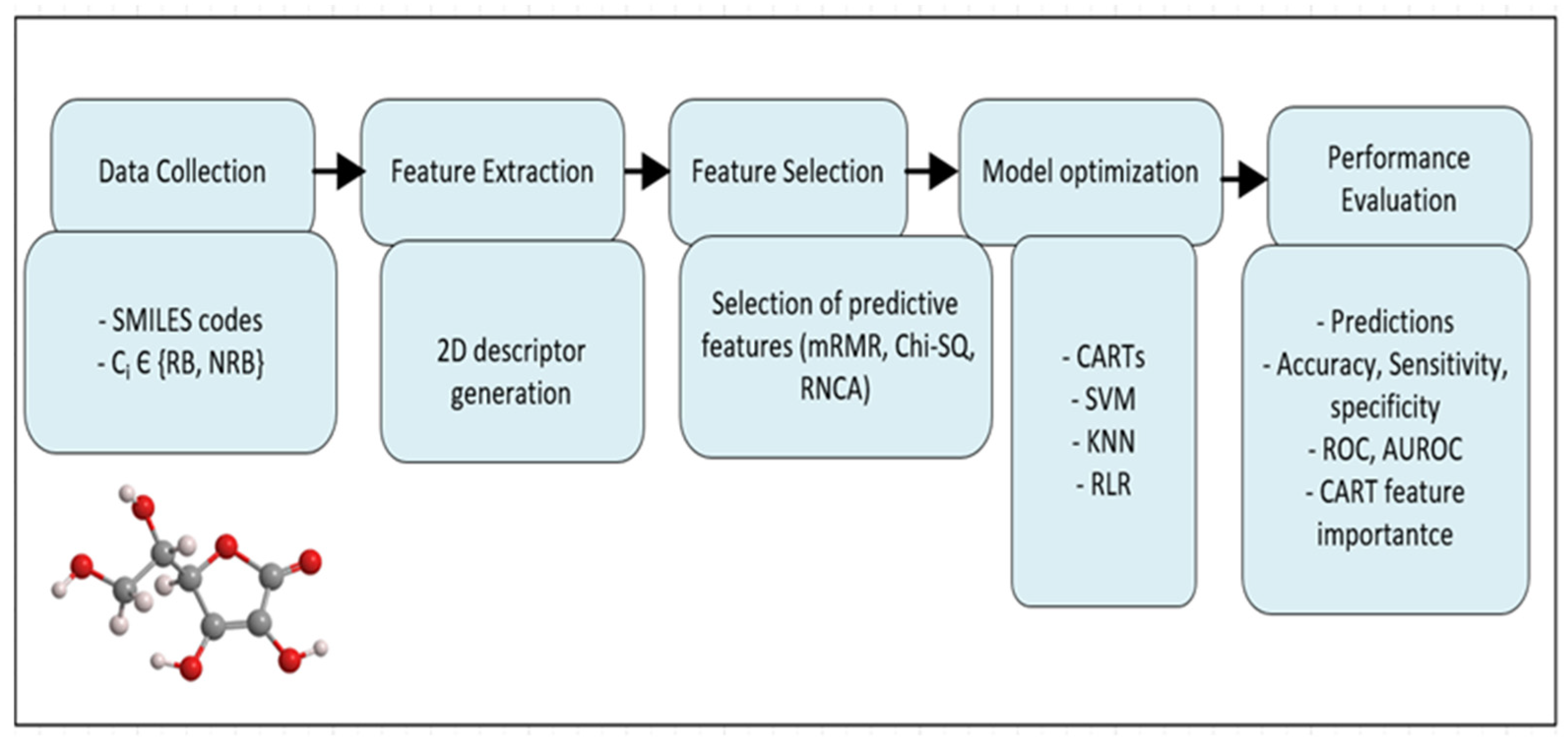
The experimental process adhered to the ELTA approach, an acronym for Extract, Load, Transform, and Analyze, in designing business intelligence solutions [35]. The ELTA approach delineates the essential stages encompassing data collection and preprocessing, feature evaluation and selection, modeling, and culminating in performance evaluation and analysis.

Figure 1 illustrates the adopted methodology. The approach began by collecting the SMILES and CAS-RN codes of biodegradation materials files from the literature. SMILES stands for simplified molecular input line entry system and CAS-RN stands for chemical abstracts service registry number. All SMILES codes were curated and checked for duplicates using alvaMolecule and the 2D dimensional descriptors were generated and filtered using alvaDesc. Constant, nearly constant, and correlated descriptors were excluded. Then, the whole dataset was partitioned into training and test subsets. Training descriptors were then provided for feature ranking using mRMR, CHISQ, and RNCA. Each ranking technique fed the three CARTs with the most predictive features one by one, and each time the cross-validation errors were calculated. The features that provided the lowest cross-validation error were selected. Then, the modeling step used the selected features to build the three CART models using the BO and repeated cross-validation algorithms [36]. Then, features were ranked according to their roles in the CART prediction process. Importance is calculated by counting how often each feature is used in splitting nodes or in surrogate splits. The performance of these CART models was compared against that obtained by SVM, kNN, and RLR. The CART models handled features with missing values using surrogate splits, but these features were imputed when building other models.

3.1. Data Collection and Preprocessing

The ready biodegradability information used in this study can be freely obtained from the literature. The dataset included the CAS-RN and SMILES codes for each chemical substance. The CAS-RN is a unique identification number assigned to distinguish individual chemical substances. It serves as an exclusive identifier that enables differentiation among various chemical substances or molecular structures, even in cases where multiple names exist. On the other hand, the SMILES code is a line notation used to represent the chemical structures of molecules. The task of assessing the biodegradability of compounds revolves around a binary classification problem, where the records are categorized as either RB or NRB substances. The original dataset was divided into three separate subsets by the data contributors. The training set contained 837 records, consisting of 284 RB and 553 NRB instances. The validation set consisted of 218 records, with 72 RB and 146 NRB instances. Lastly, the external validation set encompassed 670 records, including 191 RB and 479 NRB instances.

In this study, we applied the alvaMolecule software to check and canonicalize the SMILEs codes and the alvaDesc calculator to extract the 2D molecular descriptors. It was found that 6 training and 2 validation records were duplicated in the external validation set, so they were deleted. The three subsets were combined into one set with 1717 records with no duplications (545 RB and 1172 NRB). The alvaDesc calculator generated 4980 two-dimensional descriptors. Constant and nearly constant descriptors, as well as descriptors found to be correlated pairwise more than 98%, were excluded from further processing. This procedure removed more than half of the descriptors, leaving only 1975 features. The whole dataset was partitioned into training and test subsets with 70:30%, respectively.

3.2. Feature Selection

In machine learning, the process of feature selection holds significance as it contributes to enhancing model performance. This selection process is geared towards eliminating both redundant and noisy (misleading) features, allowing for a focus on the most pertinent ones. This approach ultimately results in more precise predictions. However, there is no single, general method for feature selection that works for all data and all models. The effectiveness of different methods depends on various factors, such as the nature of the data and the modeling task at hand. This study evaluated three common and different feature ranking techniques, mRMR, CHISQ, and RNCA.

• The mRMR algorithm processes all features to find the optimal set that differs mutually and maximally and can effectively represent the target output. The algorithm quantifies the mutual information criterion to minimize the feature redundancy and maximize the relevance of the output.
• The CHISQ evaluates the individual chi-square test result (p-value) between each predictive feature and the output. The lower the p-value between the feature and the response, the higher the importance of the feature, and vice versa.
• RNCA leverages the Mahalanobis distance measure, commonly employed in kNN classification algorithms. The primary objective is to identify the most suitable subset of predictive features that maximizes the average leave-one-out classification accuracy over the training data. To mitigate overfitting, RNCA integrates a Gaussian prior into the neighborhood component analysis objective, resulting in a regularization method that greatly enhances the generalization capabilities.

Each of these prevalent feature selection techniques presents distinct advantages, rendering them appropriate for varying scenarios and data types.

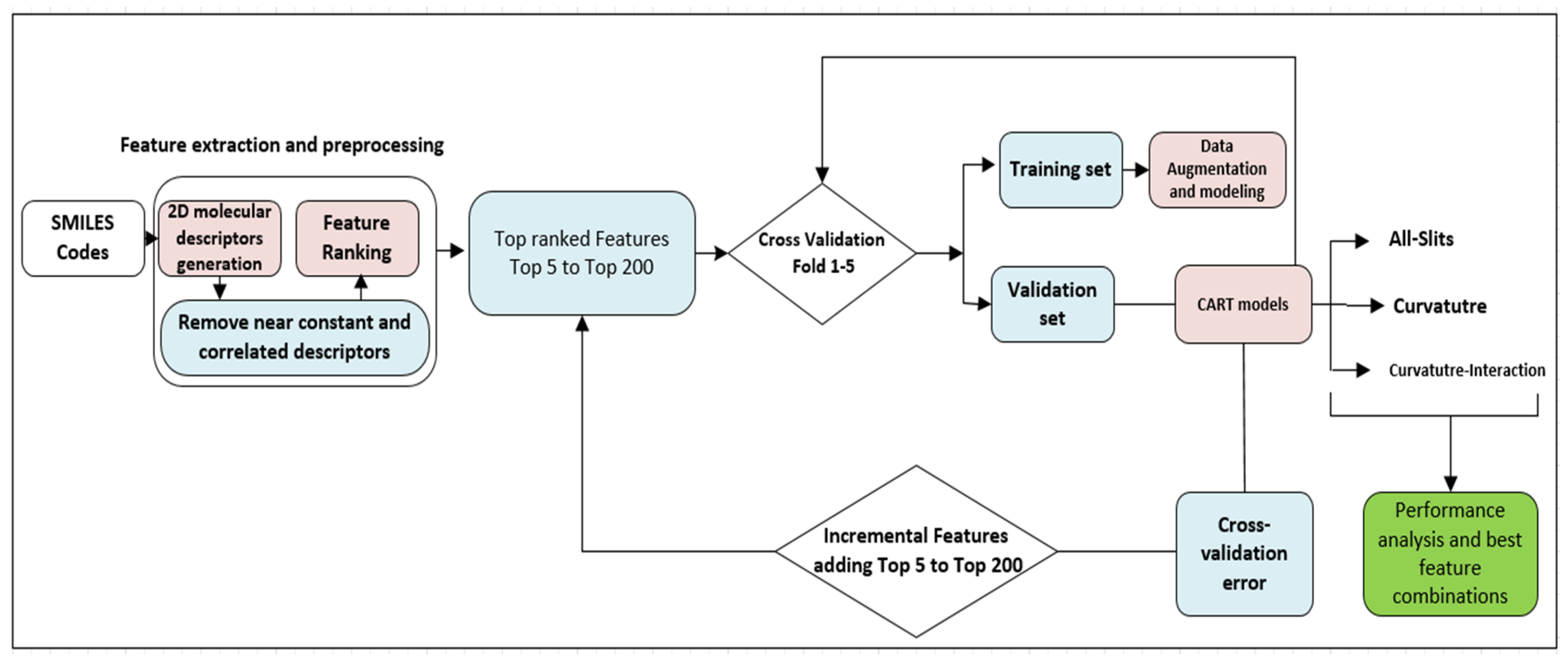
The selection process in this study followed a forward approach, as shown in Figure 2. First, features were ranked according to one of the three mentioned algorithms in descending order. Second, features were added one by one to the CART model, and each time the cross-validation error was computed and plotted. The feature set that generated the lowest error was selected to build the final CART models as well as other models, SVM, kNN, and LR.

3.3. Standard Classification and Regression Tree (CART)

Breman et al. introduced the CART model in 1984 [16], showing its effectiveness in providing effective predictive models to solve classification and regression problems. The model demonstrated its ability to identify complex associations between predictive features that are difficult or not feasible to identify using conventional multivariate methods. The main feature of the model is its transparency, as it can explain decision-making procedures clearly and understandably. The model can be represented as a tree structure where each internal node represents a test on a certain feature and each branch represents one outcome of this test. Each tree leaf represents a predicted class label. This approach enables the identification of the path from the tree’s root to a leaf node and provides insight into how a specific prediction was formulated. The CART modeling algorithm is a binary partitioning technique that divides the data in each inner node into two homogeneous subsets in the subsequent two sub-nodes (as shown in Figure 3).

The CART data partitioning process relies on a splitting criterion that measures the degree of impurity (or homogeneity) after splitting in the subsequent sub-nodes. The Gini and deviance (also called cross-entropy) are two common splitting criteria in the standard CART algorithm. For a K-class problem, the two criteria are computed as follows:

• Gini index

$$i\left(\tau \right)=1-\sum _{k=1}^K{p}_k^2$$

(1)

• Deviance index

$$i\left(\tau \right)=1-\sum _{k=1}^K{p}_k\times {\mathrm{l}\mathrm{o}\mathrm{g}}_2{p}_k$$

(2)

where p_k is the proportion of records in class k. The Gini index calculates the probability of misclassifying a randomly chosen record from the set. The deviance measures the sum of the negative logarithms of the probabilities of each class. A pure node has Gini and deviation indices of zero; otherwise, its values become positive values. The conventional CART model tends to select features that have numerous characteristic values over those with only a few. It also inclines towards selecting continuous features rather than categorical ones. If the set of predictive features is heterogeneous or if some features have significantly fewer characteristic values than others, it would be more appropriate to utilize the curvature test. Additionally, standard trees are not proficient in identifying feature interactions, and they are less likely to recognize significant features when numerous irrelevant ones are present. Hence, implementing an interaction test is crucial for the detection of feature interactions and in identifying important features when several irrelevant ones are present, as is the case in QSAR modeling.

3.4. CART with Curvature and Interaction Tests

The curvature test selects the splitting feature that minimizes the p-value of the chi-square tests of independence between each feature and the class variable. It evaluates the null hypothesis that two variables are not related. For a feature x and the output class y, the curvature test is conducted as follows.

• Numeric features are partitioned into their quartiles. They are converted into the nominal type that bins record to the quartile according to their values. An extra bin is added for missing values (if they exist).
• For every class value in y_k, k = 1,…, K, and every level in the partitioned feature x_j, j = 1,…, J, the algorithm calculates the weighted number of records in class k as follows:

$${\widehat{\pi }}_{jk}=\sum _{i=1}^{N}I\{y_i=k\}·w_i$$

(3)

where w_i represents the weight of the record i, $\sum w_i=1$; I represents the indicator function; and, finally, N represents the number of records. When all records have equal weight, then, ${\widehat{\pi }}_{jk}=\frac{n_{jk}}{N}$, where n_jk is the number of records with j feature and k class. Then, the test figure is computed:

$$t=N·\sum _{k=1}^K\sum _{j=1}^J\frac{{\left({\widehat{\pi }}_{jk}-{\widehat{\pi }}_{j+}+{\widehat{\pi }}_{+k}\right)}^2}{{\widehat{\pi }}_{j+}+{\widehat{\pi }}_{+k}}$$

(4)

where ${\widehat{\pi }}_{j+}=\sum _k{\widehat{\pi }}_{jk}$ represents the marginal (total) probability of the feature x to have the level j irrespective of the class value. Similarly, ${\widehat{\pi }}_{+k}=\sum _j{\widehat{\pi }}_{jk}$ represents the total probability of class value k. For a large record size, t is distributed as ${\chi }^2$ with (K − 1)(J − 1) degrees of freedom.

• If the p-value for the test <0.05, then the null hypothesis is rejected. The algorithm selects the splitting feature that minimizes the significant p-value (those less than 0.05). It is an unbiased selection regarding the number of levels in individual features, which provides a better interpretation of decision alternatives and a better ranking of predictive features according to their true importance. Curvature tests detect nonlinearities in the relationships between input features and the target variable and construct split points that capture the nonlinearity. This helps to improve the accuracy of predictions, particularly when the relationship between the features and target variable is complex.
• The interaction test is used to determine whether two features should be combined into a single predictor variable. The test minimizes the p-value of the chi-square tests of independence between every feature pair and the class variable. This test uses similar statistical procedures to evaluate the null hypothesis to assess the association between every pair of features for the target variable. In situations where there are several irrelevant features, interaction tests enable the identification of important features by examining the joint effect of two or more features on the target variable. Interaction tests, on the other hand, assist in identifying important features that may be overlooked by standard trees.

By incorporating curvature and interaction tests, CARTs enhance their accuracy and robustness, making them more effective in solving complex problems.

3.5. Bayesian Optimization (BO)

The BO algorithm has gained significant attention in hyperparameter tuning for various machine learning models due to its ability to reach good solutions with only a few iterations [37]. Unlike other optimization methods, the BO algorithm utilizes a surrogate function (SF) to approximate the objective function. Additionally, the BO algorithm employs another function called the acquisition function (AF) to navigate the solution space to the optimal solution efficiently. The Gaussian Process (GP) is the most popular surrogate function, and the Expected Improvement (EI) is a popular acquisition function. BO achieves this optimization through a combination of surrogate models and acquisition functions as follows.

• It starts by sampling the true objective function at some random seed points to construct the initial dataset (D₀). Then, the algorithm initializes the surrogate model SF₀.
• At each iteration t, the AF finds the point that minimizes the SF model. This point represents the best guess to record the true objective function. The input point and the resulting function value update the dataset (D_t) and the SF_t model.
• The algorithm reapplies the AF function to find the point that minimizes the updated SF_t to estimate the new candidate point and so on.
• The iteration continues several times until satisfactory information is available about the objective function and then the global minimum is obtained.

Figure 4a illustrates the concept of BO. The optimization process iteratively improves the SF model, which is then utilized to generate the best estimation for the true objective function. This guessing and recording iteration continues until the global minimum is achieved. Figure 4b demonstrates how BO, in conjunction with repeated cross-validation, optimizes the various machine learning algorithms used in this study: CARTs, SVM, kNN, and RLR.

3.5.1. Gaussian Process

The BO algorithm uses the probabilistic GP model to build a regression model of any black-box objective function f(x). The algorithm builds the surrogate GP using mean m(x) and kernel k(x, x′) functions. It serves as a prior over the space of functions that could represent the objective function. It defines a distribution over the set of functions that is consistent with the available data and can be updated as new data are observed. It is expected that objective f and its input parameters x have a common Gaussian distribution.

$$f\left(\mathbf{x}\right)~\mathcal{G}\mathcal{P}(m\left(\mathbf{x}\right),k\left(\mathbf{x},{\mathbf{x}}^{\prime }\right))$$

(5)

The mean function is set to zero for simplicity, m(x) = 0. In other words, kernel function k completely defines the GP model. The ARD 5/2 Matérn function is a conventional kernel that is a two-times differentiable function and relies on the distance between points x and x′:

$$K_{M52}\left(\mathbf{x},{\mathbf{x}}^{\prime }\right)={\sigma }_f^2\left(1+\frac{\sqrt{5}r}{{\sigma }_l}+\frac{5r^2}{3{\sigma }_l^2}\right)exp\left(-\frac{\sqrt{5}r}{{\sigma }_l}\right)$$

(6)

where $r=\sqrt{{\left(\mathrm{x}-{\mathrm{x}}^{\prime }\right)}^T\left(\mathrm{x}+{\mathrm{x}}^{\prime }\right)}$ represents the Euclidean distance between the two points, ${\sigma }_f$ represents the standard deviation, and ${\sigma }_l$ is the characteristic length scale. Their values are computed by optimizing the marginal log-likelihood of the current dataset ${\mathcal{D}}_{1:t}={\left\{\left({\mathrm{x}}_i,y_i\right)\right\}}_{i=1}^t$, where t is the iteration index. As soon as the kernel is specified, the algorithm can compute the distribution at any new location x_t+1 as follows:

$$P\left(y_{t+1}|{\mathcal{D}}_{1:t},{\mathbf{x}}_{t+1}\right)=\mathcal{N}\left({\mu }_t\left({\mathbf{x}}_{t+1}\right),{\sigma }_t^2\left({\mathbf{x}}_{t+1}\right)+{\sigma }_{noise}^2\right)$$

(7)

$${\mu }_t\left({\mathbf{x}}_{t+1}\right)={\mathrm{k}}^T{[K+{\sigma }_{noise}^2\mathrm{I}]}^{-1}{y}_{1:t}^T$$

(8)

$${\mu }_t\left({\mathbf{x}}_{t+1}\right)={\mathrm{k}}^T{[K+{\sigma }_{noise}^2\mathrm{I}]}^{-1}{y}_{1:t}^T$$

(9)

$${\sigma }_t^2\left({\mathbf{x}}_{t+1}\right)=k\left({\mathbf{x}}_{t+1},{\mathbf{x}}_{t+1}\right)-{\mathrm{k}}^T{[K+{\sigma }_{noise}^{2}I]}^{-1}\mathrm{k}$$

(10)

where $K=\left[\begin{array}{ccc}k({\mathbf{x}}_1,{\mathbf{x}}_1)& \cdots & k({\mathbf{x}}_1,{\mathbf{x}}_t)\\ ⋮& \ddots & ⋮\\ k({\mathbf{x}}_t,{\mathbf{x}}_1)& \dots & k({\mathbf{x}}_t,{\mathbf{x}}_t)\end{array}\right]; K=\mathrm{k}=[k\left({\mathbf{x}}_{t+1},{\mathbf{x}}_1\right)k\left({\mathbf{x}}_{t+1},{\mathbf{x}}_2\right)\cdots k\left({\mathbf{x}}_{t+1},{\mathbf{x}}_t\right)]$. Here, ${\sigma }_{noise}^2$ is the noise variance.

3.5.2. Expected Improvement (EI)

The BO algorithm employs a certain AF to drive the navigation towards the most promising regions of the input space. The AF should balance exploration and exploitation to efficiently optimize the objective function. In other words, it should explore regions with high variance ${\sigma }_t^2$ and exploit regions with low mean ${\mu }_t$. EI is a popular acquisition function. It calculates the expected improvement in the objective function that can be obtained by evaluating a new point x compared to the current best point x_best. EI represents the expected value of the maximum of the improvement and zero, where the improvement is defined as the difference between the predicted value at x and the current best value [38]:

$${\alpha }_{EI}\left(\mathbf{x}\right)=E\left[\max \left(0,f\left({\mathbf{x}}_{best}\right)-{\mu }_t\left(\mathbf{x}\right)\right)\right]$$

(11)

$${\alpha }_{EI}\left(\mathbf{x}\right)=\left\{\begin{array}{cc}\left(f\left({\mathbf{x}}_{best}\right)-{\mu }_t\left(\mathbf{x}\right)\right)·\Phi \left(Z\right)+{\sigma }_t\left(\mathrm{x}\right)·\Phi \left(Z\right)& \left({\sigma }_t\left(\mathbf{x}\right)>0\right)\\ 0& \left({\sigma }_t\left(\mathbf{x}\right)=0\right)\end{array}\right.$$

(12)

where $Z=\frac{f\left({\mathbf{x}}_{best}\right)-{\mu }_t\left(\mathbf{x}\right)}{{\sigma }_t\left(\mathbf{x}\right)}$ and $\Phi (·)$ is the probability density function (PDF) for the normal distribution.

EI considers both the improvement over the current best record and the uncertainty in the function values at unexplored points, which allows for a more balanced exploration–exploitation trade-off. It tends to produce higher expected improvement values, especially when the function being optimized is noisy or has a complex structure with multiple local optima [39].

4. Experimental Results

This study aimed to assess the ability of different CART models, using different splitting criteria, to classify chemical substances into either RB or NRB categories using 2D molecular descriptors. Three variations of the CART model were utilized, including the standard CART, CART with curvature, and CART with curvature–interaction feature selection criteria. Their performance was enhanced using preprocessing, feature selection, repeated cross-validation, and BO algorithms. The performance of these models was compared with that obtained for SVM, kNN, and RLR. The dataset was divided into two parts: 70% for training and 30% for testing. For model evaluation, the study employed four performance metrics: accuracy, sensitivity, specificity, and the area under the ROC curve [40].

4.1. Feature Ranking

Three distinct ranking criteria, mRMR, CHISQ, and RNCA, were employed to rank training features. Figure 5a–c illustrate the top 20 molecular descriptors according to these criteria. Specifically, Figure 5a displays the top 20 features obtained by mRMR, which is a method that identifies the most informative and least redundant set of features. The selected features have a high correlation with the classification labels and minimal correlations with each other. The algorithm strikes a balance between selecting informative features and avoiding redundant ones, resulting in a concise and effective feature subset. However, one of the most significant drawbacks of this method is its extreme sensitivity to the presence of outliers in the data, which is a common case in molecular descriptor data [41]. The top 20 features based on the CHISQ feature ranking algorithm are depicted in Figure 5b. While this method is computationally efficient compared to other criteria, it does not account for feature redundancy or interactions and does not address multicollinearity. This may result in the selection of highly correlated features, ultimately reducing the performance of the machine learning model and leading to overfitting. The top 20 features based on the RNCA algorithm are presented in Figure 5c. This algorithm serves as a wrapper feature selection technique that can prevent overfitting in scenarios where there are many records. This is due to the decrease in overfitting probability and required regularization as the number of records increases. However, a significant disadvantage of this method is its computational cost, particularly for large datasets.

For each ranking technique, datasets were extracted starting with the top five predictive features and then adding the next most important features one by one until the top 200 features were achieved. Each time, we optimized the three CART DT models using parallel Bayesian optimization. Parallel Bayesian optimization can lead to significant speedups in the optimization process when dealing with a large number of evaluations [42]. The algorithm worked with the Gaussian process as a surrogate function and the expected improvement as an acquisition function, and the maximum number of evaluations was set to 50.

Figure 6 shows the cross-validation errors of three models plotted against the number of features ranked by different selection algorithms: mRMR in Figure 6a, CHISQ in Figure 6b, and RNCA in Figure 6c. The cross-validation error is used as a measure of model generalization in data mining and machine learning. These results suggest the efficacy of combining feature selection algorithms with DT models. The plotted results suggest that raw data can have redundant features that add more calculations without improving the performance, as well as misleading features that can lead to poor performance. Therefore, it is crucial to perform feature selection to improve the performance of DT models. This conclusion regarding the importance of feature selection is illustrated more clearly in Figure 6a, in which the three trees were constructed with the five most important features and then added feature by feature according to their importance. The performance remained almost constant, and then the error suddenly decreased dramatically with 20 features; then, it continued to be stable and suddenly decreased for the second time with 50 features; it then suddenly increased as the number of features continued to increase after 70 features. It is noted that the model with curvature–interaction broke the barrier of 0.17 error and achieved almost 0.16 error. The results in Figure 5b,c do not indicate similar performance. The models’ performance fluctuated as more predictive features were added according to their respective criteria (CHISQ and RNCA). When using fewer than 40 features, the CHISQ and RNCA benchmarks performed much better than mRMR, and as more features were added, the mRMR performance improved, as discussed earlier.

4.2. CARTs: Training and Evaluation

To ensure the robustness, generalizability, and accuracy of our CART models, we utilized the mRMR feature selection, non-parallel BO, and repeated cross-validation algorithms. Throughout the optimization process, we closely monitored the cross-validation error, which served as an indicator of the model’s generalization ability (Figure 7). The classification results for both the training and testing subsets, along with the optimized hyper-parameters, are presented in

Table 1. Performance evaluation of different CART models using mRMR feature ranking technique for ready biodegradability.

Model	CV Error	Training			Testing			Model Parameters
		Acc	Sen	Sps	Acc	Sen	Sps	Split Criterion	Min Parent	Min Leaf	Max Splits
All Splits	0.18	85.36	86.65	84.76	84.66	82.82	85.51	deviance	10	2	34
Curvature	0.17	86.69	92.67	83.90	81.55	85.89	79.55	deviance	10	1	59
Curvature–Interaction	0.17	85.77	89.53	84.02	85.63	87.12	84.94	deviance	10	2	35

. The obtained results highlight the favorable and balanced performance of our models across the training and testing subsets.

While all three CART models exhibited comparable performance, the model that integrated curvature–interaction criteria showcased a slight advantage, achieving general accuracy of 85.63% on the testing subset. The CART models provide a means to quantify the importance of features by evaluating their contributions to the construction of the tree. The importance of each feature is determined by measuring the reduction in data impurity when it is used to split the data at each node of the tree. The feature’s importance score is computed by aggregating the total reduction in impurity across all splits involving this feature. A higher score indicates a more significant role in making predictions [43]. In Figure 8, the relative importance of the 60 features used in tree construction is demonstrated. The results exhibit similarities among the three models.

Notably, certain features ranked lower in importance according to the mRMR approach were assigned higher orders and greater significance in the construction of the three trees. This suggests that the ranking of feature importance derived from the filter-based approach (such as mRMR in this study) may not always reflect the absolute importance across different classification models. Among the 60 most important features identified by mRMR, several features had little to no significance in the predictions made by the CART models. Figure 8 shows that the SpMaxB(m) and SpMin1_Bh(v) descriptors stood out as significantly outperforming the others, and many features had little or no influence on the prediction process.

Table 2. Descriptive statistics of top ten features selected by three CART models.

	Range	Minimum	Maximum	Mean	Std Deviation	Skewness	Kurtosis
SpMax_B_m	15.4	2.19	17.58	3.9969	1.16114	4.318	27.649
SpMin1_Bh_v	2.33	0	2.33	1.9776	0.13717	−3.864	39.381
DLS_02	0.83	0.17	1	0.7672	0.16699	−0.461	−0.275
N_069	3	0	3	0.0957	0.35575	4.081	17.589
B05_N_N	1	0	1	0.074	0.26195	3.258	8.626
B03_N_N	1	0	1	0.0724	0.25922	3.305	8.936
NsssN	4	0	4	0.1622	0.49423	3.849	17.529
nCq	9	0	9	0.1015	0.51264	8.585	105.722
rNHR	2	0	2	0.0549	0.2891	5.636	32.251
B05_N_Cl	1	0	1	0.0333	0.17944	5.211	25.194

presents the top ten features along with their descriptive statistics, which were utilized in generating the final cost-effective CART models. The classification results of the final CART models for both the training and test subsets are presented in

Table 3. Performance evaluation of different CART models using top ten features for three CART models.

Model	cv Error	Training			Testing			Model Parameters
		Acc	Sen	Sps	Acc	Sen	Sps	Split Criterion	Min Parent	Min Leaf	Max Splits
All Splits	0.1727	84.9	86.4	84.3	84.9	84.7	84.9	gdi	10	1	29
Curvature	0.1762	84.8	87.7	83.4	84.7	86.5	83.8	‘deviance’	10	1	32
Curvature–Interaction	0.1742	84.8	86.6	83.9	85.8	85.9	85.8	‘deviance’	10	5	25

. The models demonstrated comparable performance in training classification. However, when evaluating the test results, the curvature–interaction model stood out by achieving sensitivity of 85.8%, specificity of 85.9%, and overall accuracy of 85.8%. Figure 9 illustrates the curvature–interaction CART tree that resulted from the analysis.

4.3. Model Comparisons

The performance of the proposed CART models is assessed in comparison to the three sophisticated approaches: SVM, kNN, and RLR. To optimize all models, the BO algorithm is applied twice—once utilizing the top 60 mRMR features and again solely using the top ten features selected by the CART models.

• Support vector machines (SVM) with radial basis function (RBF) kernels are widely used in machine learning for classification tasks [44]. The RBF kernel effectively separates classes in SVMs. Training an SVM with the RBF kernel requires consideration of two important parameters: C and gamma. Parameter C, common to all SVM kernels, controls the balance between training record misclassification and decision surface simplicity. A smaller C allows for a wider margin but may lead to more misclassifications, while a larger C aims to minimize misclassifications but may result in a narrower margin. The gamma parameter, specific to the RBF kernel, determines the influence of each training record on the decision boundary. A higher gamma value creates a more complex decision boundary, potentially causing overfitting, while a lower gamma value produces a smoother decision boundary, which may result in underfitting. The BO algorithm was employed to find the optimal values of C and gamma. Using the top mRMR 60 features, the study achieved general accuracies of 89.19% for the training subset and 83.30% for the test subset. In contrast, utilizing only the top 10 features recommended by the CART models resulted in accuracies of 86.94% for the training subset and 82.14% for the test subset, as shown in

  Table 4. Performance evaluation of SVM, kNN, and RLR models using top ten features for three CART models.

  Model		CV Error	Training			Testing
  			Acc	Sen	Sps	Acc	Sen	Sps
  60 mRMR features	SVM	0.15	89.19	93.46	87.20	83.30	83.44	83.24
  	kNN	0.15	100.00	100.00	100.00	83.50	81.60	84.38
  	RLR	0.19	78.04	92.41	71.34	74.18	88.34	67.61
  Top Ten Features	SVM	0.16	86.94	89.79	85.61	82.14	80.98	82.67
  	kNN	0.16	100.00	100.00	100.00	82.52	83.44	82.10
  	RLR	0.00	75.96	89.53	69.63	74.56	87.12	68.75

  .
• The K-nearest neighbors (kNN) algorithm is a popular choice in solving classification problems in machine learning [45]. It is a non-parametric, supervised learning classifier that relies on closely related features to make predictions or classifications for individual data points. In kNN, classification is based on the idea that data records with closely related features are likely to belong to the same class. The algorithm identifies the K-nearest neighbors of a given record in the feature space and assigns the class label based on a majority vote among these neighbors. The choice of K (the number of neighbors) and the distance function are crucial hyperparameters that can be tuned to optimize performance. In this study, the BO algorithm was used to determine the optimal values of K and the distance function. Using the top 60 mRMR features, the kNN model achieved accuracies of 100.0% for the training subset and 83.5% for the test subset. Similarly, when considering only the top ten features recommended by the CART models, the accuracies were reported as 100.0% for the training subset and 82.52% for the test subset, as detailed in Table 4.
• Logistic regression (LR) is a commonly used classification algorithm that models the relationships between input variables and a binary outcome using a logistic function [46]. The logistic function produces an S-shaped curve that maps inputs to a probability value between 0 and 1, representing the predicted probability of a positive outcome. The model estimates the logistic function’s parameters using maximum likelihood estimation. Regulated LR (RLR) utilizes regularization to prevent overfitting and improve generalization by adding a penalty term to the cost function. This penalty term reduces the magnitude of coefficients and prevents them from growing too large. Two popular regularization techniques in logistic regression are L1 (lasso) and L2 (ridge) regularization. L1 regularization adds the absolute values of coefficients to the cost function, causing some coefficients to become exactly zero. L2 regularization adds the squared values of coefficients to the cost function. In this study, the BO algorithm was used to find the optimal values for regularization strength (lambda) and regularization penalty type (L1 or L2). When utilizing the top 60 mRMR-selected features, the logistic regression model achieved accuracies of 78.04% for the training subset and 74.18% for the test subset. However, when considering only the top ten features recommended by the CART models, the model’s performance resulted in accuracies of 75.96% for the training subset and 074.56% for the test subset, as outlined in Table 4.

4.4. Model Evaluation Using ROC Curves

The ROC curve is an important evaluation technique for binary classification models. It provides a visual representation of a model’s performance and allows for effective comparisons between different models. The curve’s ability to handle class distribution imbalances makes it a valuable tool in various domains, such as diagnostics, medical decision-making, and machine learning. The curve is constructed by plotting the true positive rate (sensitivity) against the false positive rate (1-specificity) on a two-dimensional graph. The ROC curve is particularly useful because it allows for the comparison of different binary classification models while being unaffected by class distribution imbalances. A higher curve indicates higher sensitivity and specificity, implying better performance. Additionally, the area under the ROC curve (AUROC) is a common metric used to quantify model performance. It provides a comprehensive measure of the model’s ability to discriminate between positive and negative classes across various threshold values. AUROC ranges between 0 and 1. Higher AUROC values indicate better discrimination power, as the model exhibits higher sensitivity and lower false positive rates across different threshold settings. This performance measure is particularly useful when dealing with imbalanced datasets, where the class distribution is skewed.

Figure 10a,b depict the ROC curves of the RB class for the three CART models and Figure 10c,d show the ROC curves of SVM, kNN, and RLR, while

Table 5. AUROCs of different models for training and test subsets.

Model/AUROC	Training Subset	Test Subset
CART All Splits	0.90	0.88
CART Curvature	0.93	0.84
CART Curvature–Interaction	0.90	0.87
SVM	0.96	0.86
kNN	1	0.89
DA	0.90	0.88

records the AUROC values. The CART models achieved average training AUROCs of 0.90, 0.93, and 0.90 for the All Splits, Curvature, and Curvature–Interaction models, respectively. Similarly, they achieved average testing AUROCs of 0.88, 0.84, and 0.87, respectively. In contrast, SVM, kNN, and RLR obtained training AUROC values of 0.96, 1, and 0.90 and test AUROC values of 0.86, 0.89, and 0.88, respectively. Based on the performance on the test subset, kNN had the best performance, with 0.89 AUROC. Both DA and CART All Splits (standard CART) achieved similar performance, with 0.88 AUROC, followed by CART with Curvature–Interaction.

The study’s findings demonstrate the efficacy of the employed tools in improving CART model performance when constructing and developing efficient QSAR systems. Through the utilization of effective feature classification algorithms, suitable optimization techniques, and rigorous criteria for tree construction, it becomes possible to address issues such as overfitting and instability that may arise with decision trees.

5. Conclusions and Discussion

Biodegradability refers to the ability of a substance to be broken down by living organisms, such as bacteria and fungi. Biodegradable substances are often referred to as “environmentally friendly” as they can be broken down into harmless substances that can be recycled back into the environment. QSAR models offer many benefits for biodegradability prediction and classification. This study aimed to optimize the key advantages of CART models to develop efficient QSAR systems for the classification and feature selection of a biodegradable dataset.

The standard CART model has several key advantages in data classification tasks, including flexibility, feature selection performance, and interpretability. These characteristics make CARTs invaluable tools for physicians and medical professionals, enabling them to aggregate data and gain insights and essential knowledge. However, their performance and structure are sensitive to changes in the input data, often favoring split features with multiple distinct values and making it challenging to identify important features amidst irrelevant ones. Therefore, preprocessing and feature selection were applied to include only relevant predictive features. Unbiased trees were built using curvature and interaction tests. BO and repeated cross-validation algorithms were applied to increase the model’s generalization and enhance the model’s stability.

The proposed approach started with the curation of the SMILES codes of biodegradation materials files from the literature. The SMILES codes were then extracted and the whole dataset was partitioned into training and test subsets. Training descriptors were then provided for feature ranking using three different methods: mRMR, CHISQ, and RNCA. These rankings were evaluated and compared, and the most predictive features were selected. Three variations of the CART model were constructed: the standard CART, CART with curvature, and CART with curvature–interaction feature selection criteria. Their performance was compared to that of SVM, kNN, and RLR based on five performance metrics utilized in the study: accuracy, sensitivity, specificity, the receiver operating characteristic (ROC) curve, and the area under this ROC curve. All the models were optimized using the BO and repeated cross-validation algorithms.

The findings presented in this study highlight the promising potential of CART models in the analysis of biodegradation data, the development of an efficient and transparent QSAR classification system, and the identification of highly predictive features.

The CART model with curvature and interaction criteria exhibited the best performance. It achieved test accuracy of 85.63%, sensitivity of 87.12%, specificity of 84.94%, and a comparable area under the ROC curve of 0.87. The importance of different molecular descriptors was assessed during the decision tree classification process, and the top ten features that played a significant role in prediction were selected. Subsequently, reduced decision trees were constructed using these ten most predictive features. Among these top features, the descriptors SpMaxB(m) and SpMin1_Bh(v) were identified as outperforming the others in terms of their contributions. A concise CART tree was constructed using these top ten features, yielding remarkable results with accuracy of 85.8%, sensitivity of 85.9%, and specificity of 85.8% for the test subset. The compact tree demonstrated explanatory transparency by providing predictive decision alternatives.

In conclusion, CART models with curvature and interaction tests have proven to be a valuable tool for data analysis and biodegradation classification. These models strike a balance between interpretability and performance, making them well-suited for various QSAR applications, particularly when nonlinear relationships and interactions play a crucial role. Their ability to be graphically visualized simplifies the understanding of complex decision rules, allowing researchers to easily comprehend the model’s logic and reasoning. Additionally, they offer a feature importance ranking that can identify critical factors for interventions or further investigation. Nonetheless, researchers must carefully assess their dataset’s specific characteristics and research questions to determine whether CART with curvature and interaction tests is the most appropriate modeling approach.