Assessment of Three Major Shrimp Stocks in Bangladesh Marine Waters Using Both Length-Based and Catch-Based Approaches

Abstract

Penaeus monodon (tiger shrimp), Metapenaeus monoceros (brown shrimp), and Fenneropenaeus indicus (white shrimp) are the most economically important shrimp species in the waters of the Bay of Bengal, Bangladesh. This is the first analytical study to assess three major shrimp stocks using both length-based and catch-based methods, such as length-based Bayesian biomass estimation (LBB), length-based indicator (LBI), and a catch-based method entitled JABBA (Just Another Bayesian Biomass Assessment), to explore and process the data; estimate the growth parameters, with length at first capture; present relative biomasses; and approximate the reference points. The parameters of the von Bertalanffy Growth Function (VBGF) analysis for the tiger, brown, and white shrimps were L_∞ = 113.0 mm, 85.4 mm, and 76.4 mm, respectively, for carapace length. Our results showed that the relative biomass level (B/B_MSY) of the tiger shrimp was 0.43, suggesting an overfished status, and brown and white shrimps were 0.84 and 0.96, indicating that they were fully exploited but not overfished. This study, therefore, advised an optimum carapace length limit to catch from 57.0–70.0 mm for tiger shrimp, 44.0–53.0 mm for brown shrimp, and 40.0–48.0 mm for white shrimp. The estimated maximum sustainable yield (MSY) reference points were as follows: optimal biomass B_MSY = 3116 mt, 15,885 mt, and 2649 mt for tiger, brown, and white shrimp, respectively, and optimal harvest rate uMSY = 12%, 33%, and 8% for tiger, brown, and white shrimp, respectively. The average annual catch values for the last ten years were 265 mt, 2396 mt, and 115 mt below the estimated MSY values of 389 mt, 4899 mt, and 209 mt for tiger, brown, and white shrimp, respectively. But, brown shrimp had the estimated highest carrying capacity (31,770 mt) and intrinsic growth rate (0.66) than the tiger and white shrimp, which was replicated distinctly in the graphical representation of the Kobe plot and the surplus production plot. Hence, the brown shrimp stock is estimated to be in a better state than the tiger and white shrimp stocks.

1. Introduction

The marine fisheries sector of Bangladesh is vital to the country’s economy since it provides food and income for hundreds of thousands of marine and coastal fishers [1]. Inland capture, inland culture, and marine capture make up the country’s various fisheries resources, with marine fisheries accounting for roughly 15% of total fish production in 2020–2021. Marine shrimp accounts for 7% (46,297 mt) of overall marine fisheries production, whereas industrial shrimp trawl makes up 7% (3069 mt) of total marine shrimp production [2]. Industrial fishing through private ownership developed over the years [3], culminating in 230 such vessels engaged in fishing in the EEZ (Exclusive Economic Zone) of Bangladesh waters deeper than 40 m in 2021–2022. Of these, 28 were shrimping vessels [2]. Shrimp plays a crucial part in the country’s overall marine landings [4]. Although 37 species of shrimp have been documented from the maritime waters of Bangladesh [5,6], the tiger shrimp (Penaeus monodon), brown shrimp (Metapenaeus monoceros), and white shrimp (Fenneropenaeus indicus) are the most economically important shrimp species [1,3,6]. The tiger shrimp is superior to other species when considering economic value [7,8]. The extensive collection of post-larvae (PL) and brood stock (mature shrimp) from the wild has made the tiger shrimp fishery in Bangladesh vulnerable [8]. Contrarily, brown shrimp is a pivotal contributor to the shrimp trawling landing, accounting for more than half of the total shrimp landing [9,10]. White shrimp, the third-most-common capture from shrimp trawling, often makes up between 5 and 10 percent of the total shrimp haul [2,9].

In the early 1970s, researchers undertook a series of pilot surveys to determine the current state of the Bay of Bengal’s fish and shrimp populations. Initiated by FAO, these surveys came at the same time as the advent of a demersal trawling fleet and the completion of several stock assessments by foreign scientists working with local expertise. Using data gathered from surveys conducted between 1968 and 1971, West (1973) made an early estimate of a virgin stock of 6800–11,400 mt of shrimp biomass [11]. Rashid (1983) used Mitsui Tayo survey data from 1976–1977 to determine that the shrimp stock was 8400 mt [12]. A swept area study between 1981 and 1983 found a shrimp stock of 3600 to 3900 mt [13]. In fisheries, a target harvest rate is typically determined by calculating the Maximum Sustainable Yield (MSY) [14,15]. Historically, MSY reference points for the Bangladesh shrimp fisheries have been evaluated by applying biomass dynamic models that use catch and effort data [1,8,9,11,16,17]. However, there has been no comprehensive research on assessing life history of shrimp stocks based on the length-based approaches within the last 25 years [18], beyond graphical presentation of length–composition and length–weight data of species groups of several cruises in different years, which have been included as length-based status in the survey report of RV Meen Sandhani [5]. But, the conducted surveys were seasonal on an intermittent basis. Hence, applying length-based stock assessment methods on such length–frequency data should be regarded with caution if the data are not representative throughout the entire year. The common assumption of any length-based package is that the data should be representative [19,20,21]. In addition, a study on shrimp species by Mustafa et al. (2006) used the traditional length-based fish stock assessment (FiSAT-The FAO-ICLARM Stock Assessment Tools) technique [18]. But, Sparre (1990) mentioned that length-converted catch curves of traditional length-based methods cannot be used for short-lived animals when growth is seasonal, including penaeid shrimps, which have more than one cohort in a year [22].

Though the number of shrimp trawlers has remained the same for the last two decades, overall shrimp landings have declined since the fishery began from the mid-eighties [9]. Due to their high monetary value and demand, these fisheries require careful management based on expert scientific advice assembled from a comprehensive stock assessment strategy. Detailed information on historical catch data, mortality, age structure, stock–recruitment relationship, catch-per-unit effort, and other life-history parameters are all crucial for a conventional stock assessment [23]. Marine fisheries in Bangladesh are categorized as data-poor because they lack this information. This is in line with most of the world’s fish stocks. The fundamental indices of abundance needed for these approaches are dependent on catch and effort data [24,25], although various data-poor stock assessment methods based on surplus production models (SPMs) have been developed [26,27,28]. However, these indices can be inconclusive and/or misleading using a single assessing approach in relation to having information about the status of stock using a variety of methodological approaches [29,30].

In this study, we tried to figure out the status of the three commercially important shrimp species stocks in the marine waters of Bangladesh by using the most up-to-date analytical tools based on both length-based and catch-based methods. Compared to the findings of earlier studies, the results are interpreted in the context of formulating sustainable management measures.

2. Materials and Methods

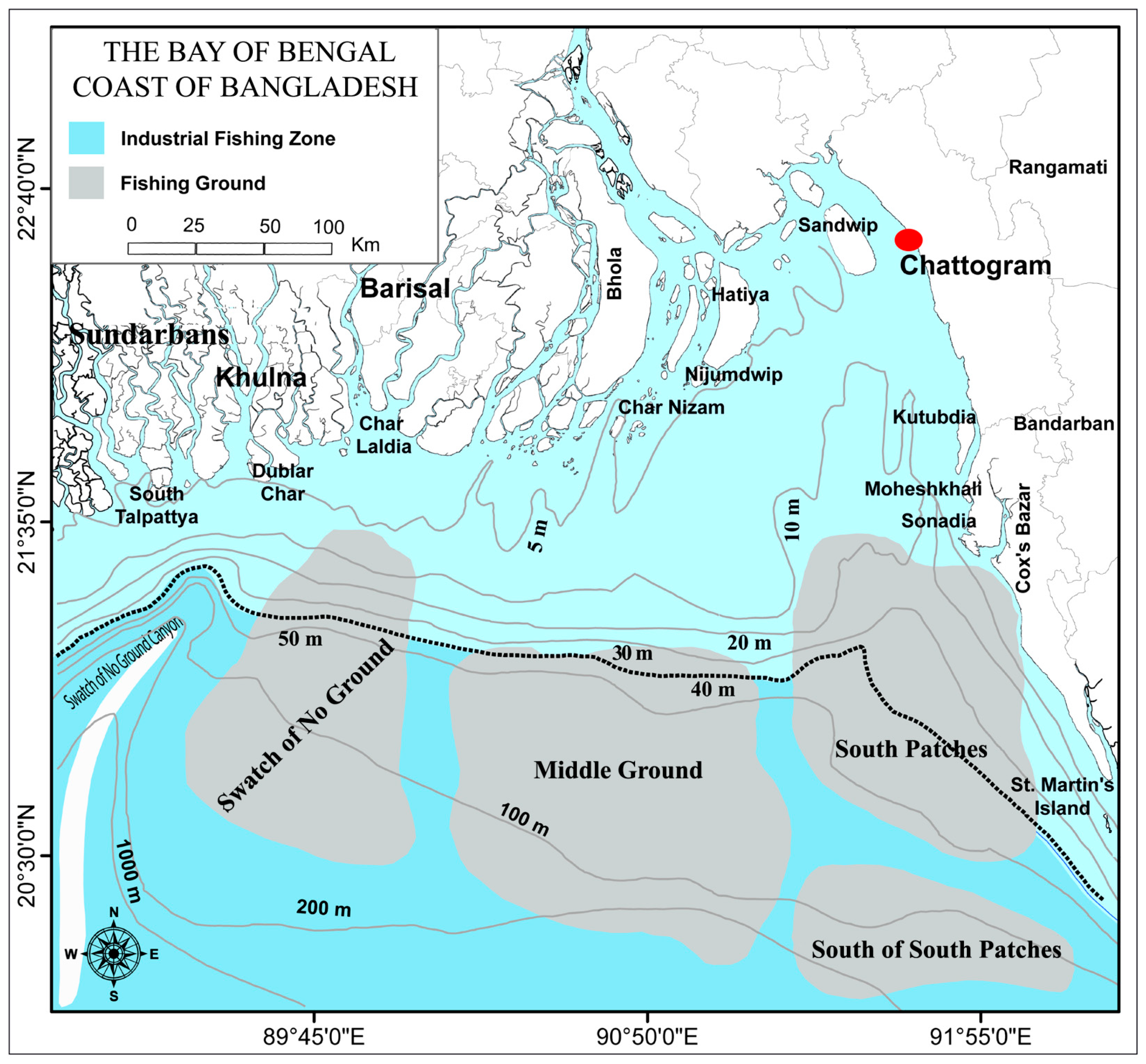
2.1. Study Area

The marine fisheries sector of Bangladesh consists of two sub-sectors: industrial and artisanal. Industrial fishing has been earmarked to fish no shallower than 40 m depth by law [31,32] in the EEZ of Bangladesh (Figure 1). Industrial trawlers are of two kinds, including freezer and iced wooden-hull trawlers. Freezer trawlers are divided into shrimp and finfish trawlers [33,34]. The overall lengths (LOAs) of shrimp trawlers are from 20.5 to 44.5 m, they have outriggers, and they operate 2–4 modern shrimp nets at a time. The mesh sizes of the cod end of the shrimp trawl nets has been allowed to fix at 45 mm, and the head rope lengths were from 15 to 35 m [35]. Shrimp trawler capacities usually have a gross tonnage of 150–250 metric tons with a main engine power of 500–900 HP. Thirty (30) days of fishing have been allowed by law on each trip. The usual number of hauls is 5–6 on a fishing day, and the period of each haul is 3–4 h. The fishing days and the number of hauls vary based on weather conditions and the vessel’s seaworthiness [1].

2.2. Data Sources

2.2.1. Length-Based Methods

Length frequency data of carapace length (CL) (head length) from 1496 individuals of tiger shrimp (both sex), 1365 individuals of brown shrimp (both sex), and 1084 individuals of white shrimp (both sex) were collected (Figure 2) monthly from July 2021 to May 2022 from industrial shrimping trawlers, except in June 2022, due to the annual fishing ban [31]. During length measurement, data collecting crews specified by the skipper of the shrimping vessels randomly collected 10% of well-mixed shrimp from each category while a sufficient number of samples were hauled. Otherwise, take the whole catch to measure for the small amount of catch. Landings were very poor for white shrimp in March, April, and May. Carapace lengths were measured to the nearest 0.1 mm using digital slide calipers for the three abovementioned shrimps.

2.2.2. Catch-Based Methods

Though trawl fishery commenced in 1972 [3], commercial shrimp trawling achieved its pace in 1986 [35]. Therefore, to analyze the stock status from catch and resilience, the time-series data (catch and effort) from 1986 to 2021 (36 years) of commercially important shrimp species of P. monodon, M. monoceros, and F. indicus were taken from logbook data sheets of the marine fisheries office of Department of Fisheries (DoF) and Fisheries Resource Survey System’s (FRSS) publication [9].

2.3. Stock Assessment Indicators

For the inclusive assessment of three major industrial shrimp stocks, we first used a newly developed R package, length-based Bayesian Biomass Estimation, known as LBB of Froese et al. (2018) to assess the fishery’s biological characteristics (growth and ratio of mortality), exploitation, and selectivity [21].

Secondly, we incorporated length frequency (LF) data into the length-based sustainability indicators proposed by Froese (2004) with respect to length reference points [37,38]. These indicators estimated a parameter that prevented growth and recruitment overfishing based on management recommendations.

Finally, we used Winker et al. (2018)’s Just Another Bayesian Biomass Assessment (JABBA) to assess catch–effort time-series data to give an innovative biomass dynamic modeling approach [39].

2.3.1. LBB Method

Froese et al. (2018) introduced a new and straightforward method, LBB (Length-based Bayesian Biomass Estimation), to assess stock status by analyzing length frequency data from commercial catches [21]. Species that grow throughout their lives, as do most commercially exploited fish and invertebrates, are suitable for the LBB approach, which requires only length–frequency (LF) data. It can elucidate asymptotic length (L_∞), mean length at first capture (L_c), relative natural mortality (M/k), and relative fishing mortality (F/M) from one or more LF samples of a stock’s size composition [21,40]. In the LBB, the assumption is growth in body length according to the von Bertalanffy (1938) growth equation [41], which can be described as:

$$L_t=L_{inf}\left[1-e^{-k(t-t_0)}\right]$$

(1)

L_t is the length at age t, L_∞ is the asymptotic length, k is the rate by which L_∞ is approached, and t₀ is the theoretical age at zero length.

For full gear selection, catch curve is expressed by the equation [15]:

$$N_L=N_{L_{start}}{\left(\frac{L_{inf}-L}{L_{inf-L_{start}}}\right)}^{\raisebox{1ex}{$z$}\!\left/ \!\raisebox{-1ex}{$k$}\right.}$$

(2)

where $N_L$ is the number of survivors to a specific length L, $N_{L_{start}}$ is the number at length L_start with full selection (i.e., the gear retains all individuals entering the gear), Z is the total mortality rate, and k is the somatic growth rate.

The selectivity of the fishing gear (here is assumed to be a trawl selection curve) can be given as the function:

$$S_L=\frac{1}{1+e^{-⍺\left(L-L_c\right)}}$$

(3)

where S_L is the fraction of individuals that are caught by the gear at length L, L_c is the length at first capture, and ⍺ denotes the steepness of the ogive [15,42].

The life history parameters of L_∞, L_c, ⍺, M/k, and F/k and the selection ogive are calculated by applying the following two equations [40]:

$$N_{L_i}=N_{L_{i-1}}{\left(\frac{L_{inf-}{L}_i}{L_{inf-}{L}_{i-1}}\right)}^{\frac{M}{K}+\frac{F}{K}{S}_{L_i}}$$

(4)

$$C_{L_i}=N_{L_i}{S}_{L_i}$$

(5)

where $N_{L_i}$ is the number of L_i length class individuals, $N_{L_{i-1}}$ is the number of individuals in the previous length class, and $C_{L_i}$ is the catch for length class L_i [21]. The ratio of M/k and F/M are not the absolute values of F, M, and k to minimize the parameter requirements. Then, M/k and F/k can be deduced by fitting Equation (4) to LF data.

The length L_opt, representing the maximum biomass of the unexploited cohort [43], is obtained from:

$$L_{opt}=L_{inf}(\frac{3}{3+\frac{M}{K}})$$

(6)

Based on Equation (6), the mean length at first capture (L_{c_opt}), which maximizes the catch and the biomass for a given pair of F/M and M/K ratios, is expressed by the equation:

$$L_{c\_opt}=\frac{L_{inf}(2+3\frac{F}{M})}{(1+\frac{F}{M})(3+\frac{M}{K})}$$

(7)

As per Hordyk et al. (2015) and Froese et al. (2018), to simulate the estimation of L_c and L_inf, the M/K value was set to 1.5 [20,21]. Using this equation, we can determine the Z/K prior (the ratio of the total mortality rate to the somatic growth rate) [15,44]:

$$\frac{Z}{K}=K(\frac{L_{inf}-L_{mean}}{L_{mean}-L_c})$$

(8)

F/K prior equals Z/K-M/K, and the relative fishing mortality F/M = (F/K)/(M/K).

According to Froese et al. (2018) [21], the relative yield per recruit (Y’/R) and catch per unit effort per recruit (CPUE’/R) specified by Beverton and Holt in 1966 [45] can be calculated as a function of Lc/Linf, F/K, M/K, and relative fishing mortality (F/M). Assuming CPUE is proportional to biomass in the exploited population, the derived index of CPUE’/R indicates the utilized biomass per recruit B’/R. The relative biomass of fish (>L_c) when no fishing occurs (F = 0) is expressed as:

$$\frac{B_{0\prime }>L_c}{R}={\left(1-\frac{L_c}{L_{inf}}\right)}^{\frac{M}{K}}(1-\frac{3\left(1-\frac{L_c}{L_{inf}}\right)}{\left(1+\frac{1}{\raisebox{1ex}{$M$}\!\left/ \!\raisebox{-1ex}{$K$}\right.}\right)}+\frac{{3\left(1-\frac{L_c}{L_{inf}}\right)}^2}{\left(1+\frac{2}{\raisebox{1ex}{$M$}\!\left/ \!\raisebox{-1ex}{$K$}\right.}\right)}-\frac{{\left(1-\frac{L_c}{L_{inf}}\right)}^3}{\left(1+\frac{3}{\raisebox{1ex}{$M$}\!\left/ \!\raisebox{-1ex}{$K$}\right.}\right)})$$

(9)

when B₀′ is the unfished biomass, the ratio of fished to unfished biomass is:

$$\frac{B}{B_0}=\frac{\left(\frac{{CPUE}^{\prime }}{R}\right)}{\left(\frac{B_0>L_c}{R}\right)}$$

(10)

The relative biomass that can produce proxy MSY ($\frac{B_{MSY}}{B_0}$) for a given fishery can be evaluated by re-running Equations (9) and (10) with $\frac{F}{\mathrm{M}}=1$ and L_c = L_{c_opt} [21].

All the analysis was performed using LBB_33a.R, an R-code algorithm presented by Froese et al. (2018) [21] (http://www.oceanrep.geomar.de/ accessed on 10 November 2022). The estimated value of $B/B_{MSY}$ classifies the status of stock; overexploited status is assigned where $B/B_{MSY}$ < 0.8, fully exploited status is where 0.8 ≤ $B/B_{MSY}$ ≤ 1.2, and non-fully exploited status is where $B/B_{MSY}$ > 1.2 [46].

2.3.2. Length-Based Indicators

Three candid length-based indicators (P_mat, P_opt, and P_mega) were suggested by Froese (2004) to maintain fishing sustainability and minimize growth and recruitment overfishing [37].

P_mat and P_opt with 100% as the target display the proportion of fish that are mature and the ideal size in the catch, and P_mega shows the proportion of mega-spawners in the catch, defined as fish higher than the length of optimum (L_opt) plus 10% of L_opt (≥1.1% L_opt). The targeted length classes should fall between L_opt and ±10% of L_opt to maintain the fishery’s sustainability and optimum biological yield. These indicators can, therefore, be calculated as:

$$P_{mat}={\sum }_{Lmat}^{Lmax}\left(P_L\right)$$

(11)

i.e., the percentage of fish in the catch having a length greater than the length at sexual maturity (L_m).

$$P_{opt}={\sum }_{L0.9Lopt}^{1.1Lopt}\left(P_L\right)$$

(12)

i.e., the percentage of fish between 0.9 × $L_{opt}$ and 1.1 × $L_{opt}$ where log($L_{opt}$) = 1.053 × log(lm) − 0.0565.

$$P_{mega}={\sum }_{1.1Lopt}^{Lmax}\left(P_L\right)$$

(13)

i.e., the percentage of fish greater than 110% of the optimum length (≥1.1$L_{opt}$), where $P_L$ indicates the percentage of fish in the catch in the length interval L.

2.3.3. Fisheries Reference Points from Catch Data

These three commercially important shrimp species are usually ready to export from shrimping vessels, and this is why the prevalence of the under-reporting of shrimp catches is thought to be low. Headless shrimps of the three studied species are mainly exported, except for some head-on tiger shrimps. Conversion factors of 0.63 for tiger shrimp, 0.66 for brown shrimp, and 0.68 for white shrimp were used to convert catch data from headless weight to total weight [1]. The catch is expressed in metric tons (mt), and effort is calculated as the sum of all fishing days across all vessels.

The JABBA Model

The JABBA model, which stands for “Just Another Bayesian Biomass Assessment,” is a Bayesian State-Space Surplus Production Model (SPM) that uses data weighting and a state space tool to fit and average many CPUE time-series data. This approach makes the ability to select among the Fox, Schaefer, or Pella–Tomlinson production functions. It offers choices for assessing or correcting process and observation errors as well as future projections to determine the proper catch regime needed to improve stock biomass [39].

SPMs are some of the most straightforward and popular models for describing the capture of excess or surplus biomass from fish stock. In its simplest terms, fish growth and reproduction increase the size of the stock, and, in contrast, natural and fishing mortality reduce the size of the stock. Though its applications have often been questioned, the stock production model has been an accepted fishery management strategy to estimate the Maximum Sustainable Yield (MSY) [14,15].

Most crucially, these models do not require size or age information [28,39]. Empirically, the changes in biomass over time, which are prone to variations in size structure, recruitment, selectivity, environmental circumstances, etc., are often not effectively described by SPMs [47]. As a result, uncertainties in parameter estimation are typical to observe. However, Bayesian state-space modelling techniques in SPMs address process errors (biomass dynamics variability) and observation errors (biomass index variability) to reduce model parameter uncertainty [39].

The generalized three-parameter SPM proposed by Pella and Tomlinson (1969) is used to define the surplus production function in this model as follows [47]:

$${SP}_t=\frac{r}{\left(m-1\right)}{B}_t(1-{(\frac{B_t}{K})}^{m-1})$$

(14)

where r, K, and B are the intrinsic rate of population growth, carrying capacity, and the biomass of the stock at time t, and m is the shape parameter that determines the B/K ratio for maximum surplus production.

The Schaefer form is used when the shape parameter (m) is 2, with surplus production reaching MSY at K/2 [39]. If 0 < m < 2, surplus production causes MSY at biomass levels below K/2 and vice versa if m > 2. The Pella–Tomlinson model maximizes excess production at 0.37 K when m approaches one through Fox models [48]. Therefore, B_MSY can be estimated from the following equation:

$$\frac{B_{MSY}}{K}=m(-\frac{1}{m-1})$$

(15)

From Equations (14) and (15), B_MSY and fishing mortality at MSY (F_MSY) can be calculated:

$$B_{MSY}=Km(-\frac{1}{m-1})$$

(16)

$$F_{MSY}=\frac{r}{m-1}(1-\frac{1}{m})$$

(17)

From a fisheries basic equation C = FB, fishing mortality is then expressed as

$$F=\frac{C}{B}$$

(18)

where C is the annual catch. Therefore, MSY can be depicted as

$$MSY=F_{MSY}.B_{MSY}$$

(19)

By combining and rearranging Equations (16)–(18), it is possible to express r in Equation (14) as:

$$r=\frac{MSY}{B_{MSY}}.\frac{m-1}{1-\frac{1}{m}}$$

(20)

Equations (16) and (20) show the possibility of converting MSY/B_MSY and B_MSY/K estimates into r and m [49,50].

Additionally, JABBA permits surplus production and a standard “hockey stick” recruitment function. Barrowman and Myers (2000) [51] introduced the hockey stick model, which states that recruitment potential is considerably stalled below a specific biomass ratio level: P_lim = B_lim/K, with P_lim values of 0.2–0.25 commonly used as recruitment overfishing limits [39]. Including a multiplier into the surplus production function makes it possible to achieve a linear reduction in the underlying hockey stick between 1 and 0. For values of B/K < P_lim:

$${SP}_t=\frac{r}{\left(m-1\right)}\frac{B_t}{\left(P_{lim}K\right)}{B}_t\left(1-{\left(\frac{B_t}{K}\right)}^{m-1}\right)if \frac{B_t}{K}<P_{lim}$$

(21)

This composite model becomes the Pella–Tomlinson model as $P_{lim}$ approaches zero.

Input Fishery Data

JABBA requires two comma-separated value files (.csv). The “Catch” input file contained the time-series shrimp catch (mt) of industrial trawlers from 1986 to 2021, and the “Abundance indices” file included the CPUE for those years.

Formulation of Input Parameters

JABBA investigates stock status using catch and abundance indices (CPUE) and the priors of initial carrying capacity (K), intrinsic rate of population increase (r), and starting biomass depletion rate (psi). The initial model run assumed that K was ten times the maximal catch in the time-series data, with a coefficient of variation (CV) of 200% [52]. For r, the general range based on SealifeBase’s resilience categories [27] was used. Commercial-scale shrimp collecting in Bangladesh’s coastal waters began in the 1980s [9]. Therefore, assuming that the stock’s initial biomass was near its carrying capacity (K) with a CV = 0.25, the lognormal biomass depletion prior (psi) for the base model was set at 0.9 K. While the process variance and observation variance priors were implemented by assuming the inverse gamma distributions specified by Winker et al. (2018), all catchability parameters were expressed as non-informative homogeneous priors [39].

This study employed the JABBA default option for process variance priors, which was σ²_Δ~1/gamma (4, 0.01). This study had a process error mean of 0.059, 95% confidence ranges of 0.03–0.1, and a CV of 28% [53]. State-space SPMs worked best at this process error level [39]. The observation variance was made up of an observation error that could be estimated externally (σ_SE) with changes in catchability from year to year [39]. It is usual to add a fixed observation error for abundance indices with externally generated standard errors to account for additional sampling errors [54]. Total observation errors between 0.1 and 0.4 were assumed for abundance indices [39].

3. Results

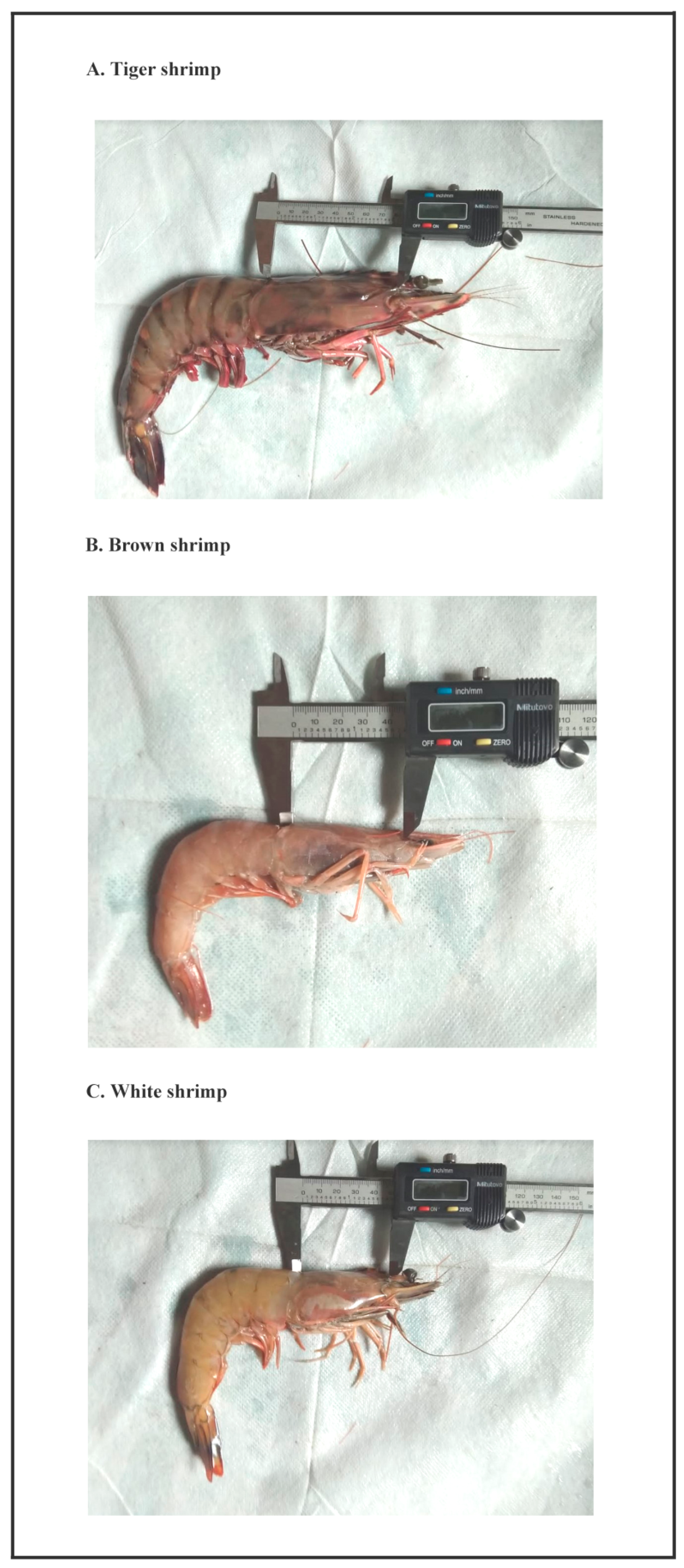
3.1. Length Distribution

Length frequency composition (Figure 3) for three shrimp species displayed a length range of carapace length (CL) from 38.0 to 120.0 mm for tiger shrimp, 18.0 to 74.0 mm for brown shrimp, and 28.0 to 75.0 mm for white shrimp.

The median length of the tiger shrimp was 79.0 mm, the brown shrimp was 46.0 mm, and the white shrimp was 51.5 mm (

Table 1. The number of individuals in the monthly sample collections from July 2021 to May 2022.

Species	Month											Total
	Jul’21	Aug’21	Sep’21	Oct’21	Nov’21	Dec’21	Jan’ 22	Feb’22	Mar’22	Apr’22	May’22
Tiger shrimp	100	90	105	180	351	125	129	130	100	113	73	1496
Brown shrimp	90	90	105	183	183	122	119	155	100	138	80	1365
White shrimp	98	90	105	90	219	102	90	95	67	64	64	1084

).

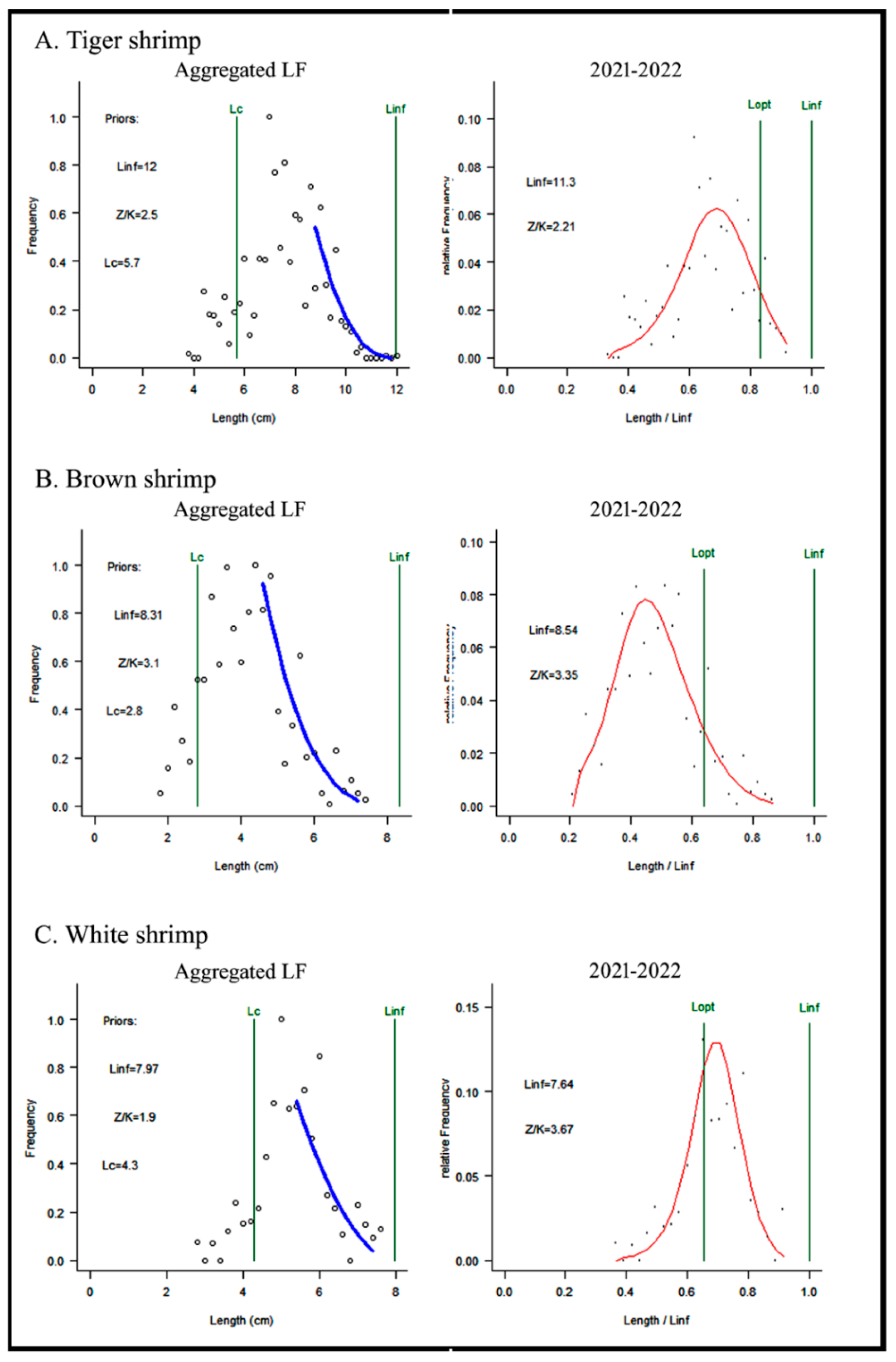
3.2. Shrimp’s Stock Analysis Based on LBB Outputs

Results of LBB estimation (

Table 2. Summary of LBB estimates for three commercial shrimp stocks.

Parameter	Tiger Shrimp	Brown Shrimp	White Shrimp
$L_{max}$ (mm)	120.0	74.0	75.0
$L_{mean}$ (mm)	90.8	45.2	57.1
$L_{inf}$ (mm)	113.0 (111.0–116.0)	85.4 (84.0–87.0)	76.4 (74.0–78.6)
$L_{c50}$ (mm)	72.6 (71.2–74.0)	33.3 (32.5–34.0)	51.0 (50.3–51.6)
$L_c/L_{c\_opt}$	0.85	0.73	1.2
$L_{mean}/L_{opt}$	0.9	0.84	1.2
$L_c/L_{inf}$	0.64 (0.63–0.65)	0.39 (0.38–0.40)	0.66 (0.65–0.67)
$L_{95th}/L_{inf}$	0.92	0.87	0.92
$M/k$	0.61 (0.35–0.83)	1.68 (1.4–1.97)	1.59 (1.35–1.86)
$F/M$	2.6 (1.5–5.1)	0.99 (0.7–1.4)	1.31 (0.74–1.94)
$Z/K$	2.1 (1.8–2.6)	3.3 (3.1–3.6)	3.7 (2.9–4.4)
$B/B_0$	0.18 (0.06–0.37)	0.3 (0.18–0.45)	0.35 (0.14–0.56)
$B/B_{MSY}$	0.43 (0.14–0.87)	0.84 (0.5–1.2)	0.96 (0.39–1.6)
alpha	1.28 (1.24–1.32)	2.0 (1.92–2.09)	2.89 (2.79–2.99)
Status	Grossly overexploited	Fully exploited but not overfished	Fully exploited but not overfished

) using length–frequency (LF) data of 3945 individuals for three commercially important shrimp species from Bangladesh marine waters were given below.

3.2.1. Tiger Shrimp

Tiger shrimp is widely distributed around Bangladesh’s coastal and marine waters. This species was observed to reach the maximum carapace length or head length of 120.0 mm. The estimate of B/B₀ = 0.18 indicates that the present condition of biomass is deficient, i.e., the stock has declined by 82% from its original level (Figure 4A), whereas the estimate of F/M = 2.6 denotes that tiger shrimp is largely overfished. The ratio of $L_{mean}/L_{opt}$ (=0.9) and $L_c/L_{c\_opt}$ (=0.85) are below unity, indicating fishing of small individuals that leads to the chance of growth overfishing. The ratio of B and $B_{MSY}$ ($B/B_{MSY}$) was 0.43, which indicates that the stock is grossly overexploited.

3.2.2. Brown Shrimp

The major shrimp catch in the shrimping vessel was brown shrimp. This species reached a maximum carapace length of 74.0 mm. The estimated parameters $F/M$ (=0.99) and $B/B_0$ (=0.47) indicated that the stock was in good condition (Figure 4B). In addition, the ratio of B and $B_{MSY}$ ($B/B_{MSY}$) was 0.84, which denoted that the stock was in the fully exploited condition but not overfished, indicating the stock was sustainable.

3.2.3. White Shrimp

White shrimp is widespread around the Indo-pacific subcontinent. It reaches a maximum length of 75.0 mm. In this study, the $F/M$ (=1.3) indicates that the fishery is under increasing fishing pressure. The ratio $B/B_0$ (=0.35) is very low, projecting that its standing biomass has declined significantly. The ratio parameters $L_{mean}/L_{opt}$ (=1.2) and $L_c/L_{c\_opt}$ (=1.2) are above unity, which suggests that the size of white shrimp is still in a good condition. Although, the stock is in a fully exploited ($B/B_{MSY}$ = 0.96) condition (Figure 4C).

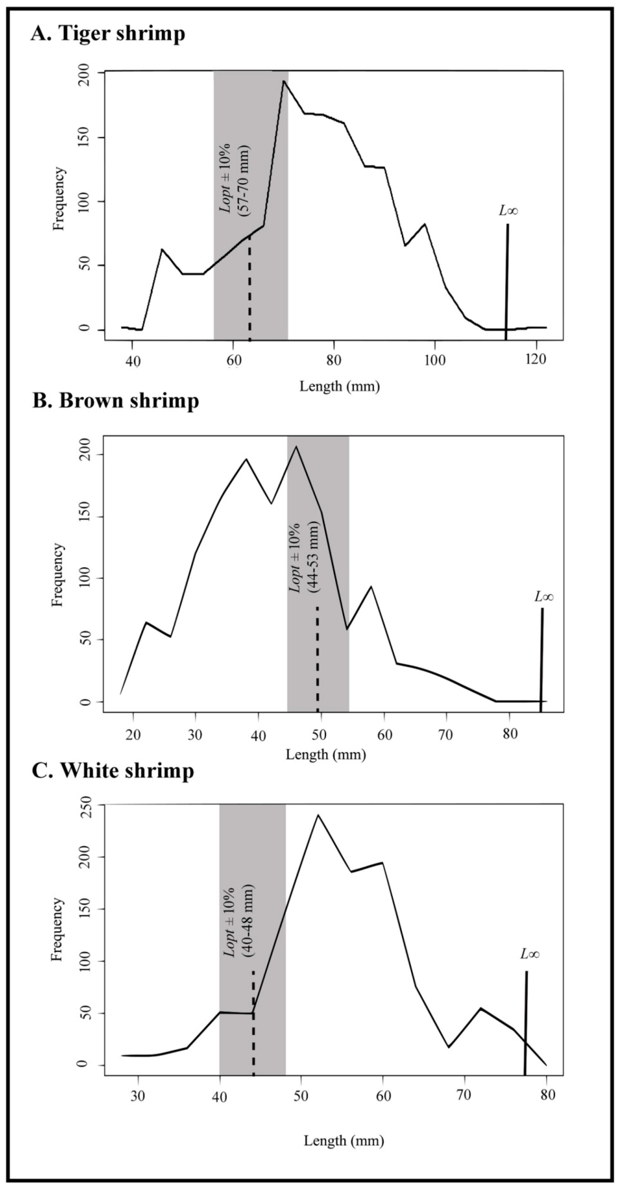
3.3. Results from Length-Based Indicators

According to the catch composition analysis, only 25.13 percent, 30.69 percent, and 20.02 percent of the shrimp were of an optimum size (P_opt) for tiger, brown, and white shrimp, respectively, whereas 86.09%, 35.53%, and 92.06% of the shrimp were of mature size (P_mat) for those species. The proportions of older and larger shrimp, known as mega-spawners (Pmega), were 63.03% for tiger shrimp, 13.19% for brown shrimp, and 73.89% for white shrimp (

Table 3. The results of LBI (length-based indicators) are based on the indicators and a decision tree proposed by Froese (2004) and Cope and Punt (2009) [37,38], respectively.

Species	Lm (mm)	Lopt (mm)	Pmat	Popt	Pmega	Pobj	Stock Condition	Probability of Being SB < RP
Tiger shrimp	113.0	63.43	86.09	25.13	63.03	1.74	SB < RP	44% for TRP 22% for LRP
Brown shrimp	85.4	48.67	35.53	30.69	13.19	0.79	SB ≥ RP	0% for TRP 0% for LRP
White shrimp	76.4	43.8	92.06	20.02	73.89	1.86	SB < RP	44% for TRP 22% for LRP

Note: SB is the spawning biomass, RP is the reference point, TRP is the target reference point, and LRP is the limit reference point.

). Maximizing marine shrimp fisheries’ production requires targeting the length classes (L_opt ± 10% of L_opt) between 57.0–70.0 mm for tiger shrimp, 44.0–53.0 mm for brown shrimp, and 40.0–48.0 mm for white shrimp (Figure 5).

Based on Cope and Punt’s (2009) decision tree [38], there is no (0%) probability that the true spawning biomass (SB) could be below both TRP and LRP for brown shrimp among the three studied shrimp species, which indicated a healthy spawning stock biomass of brown shrimp in the marine waters of Bangladesh.

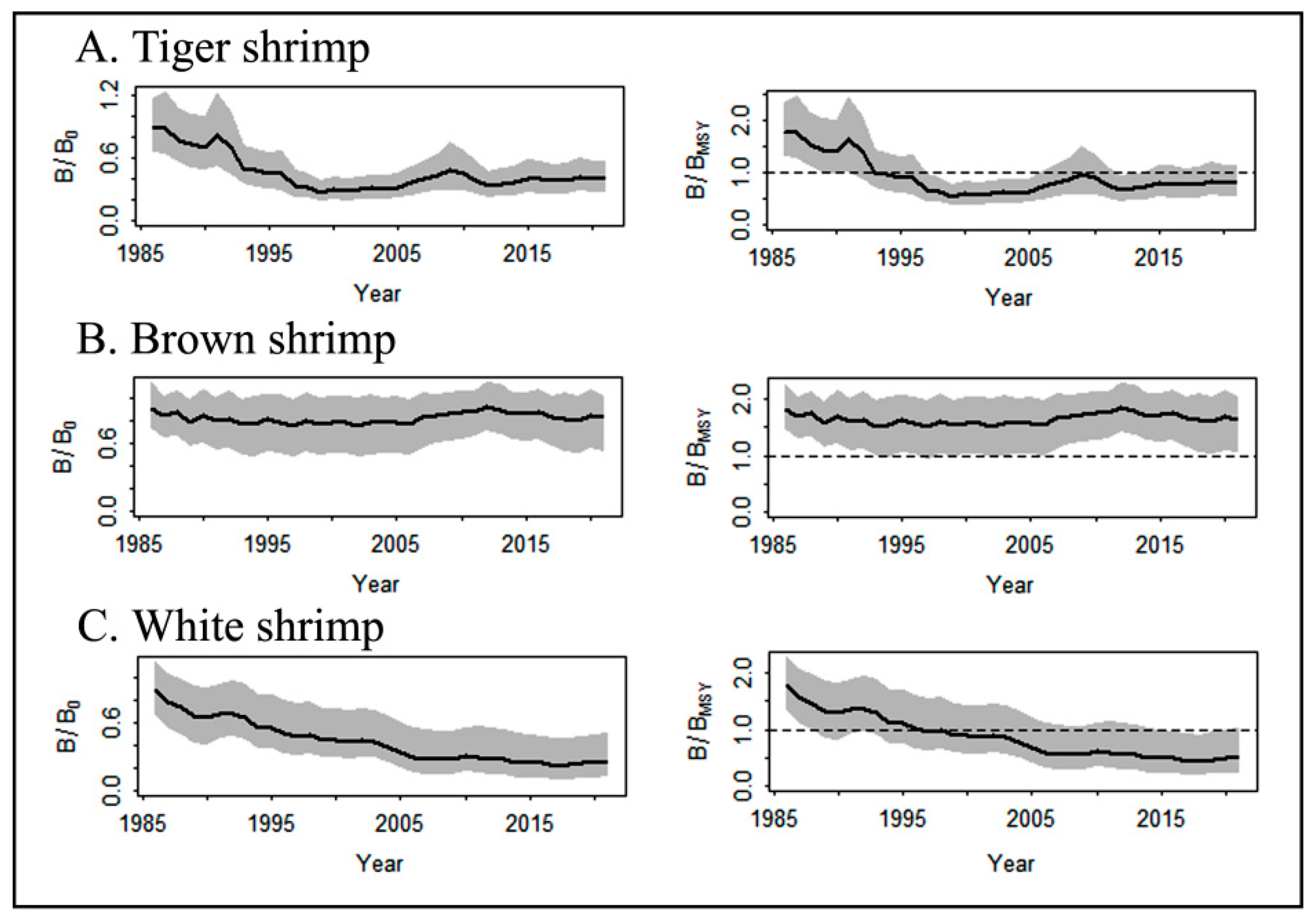
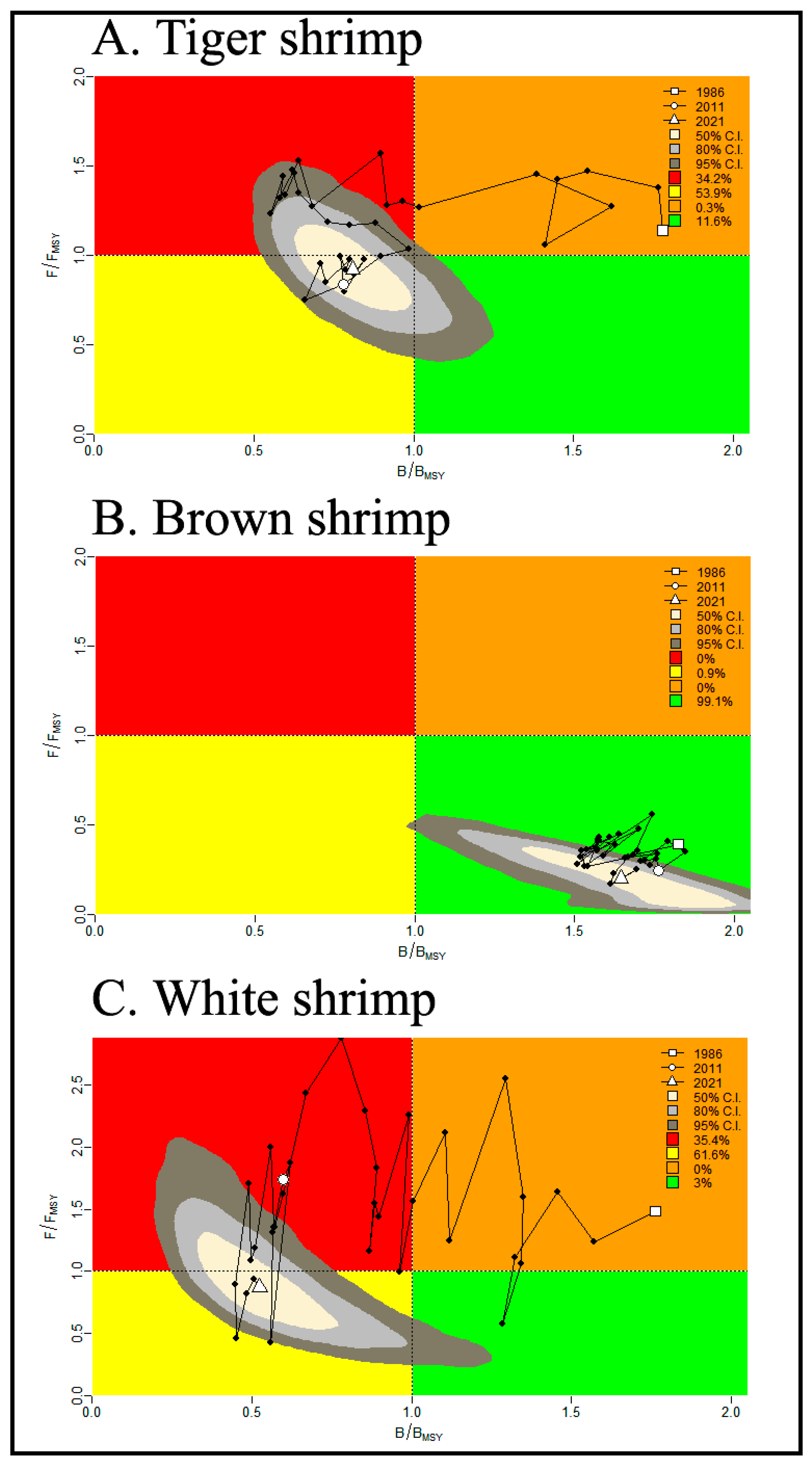
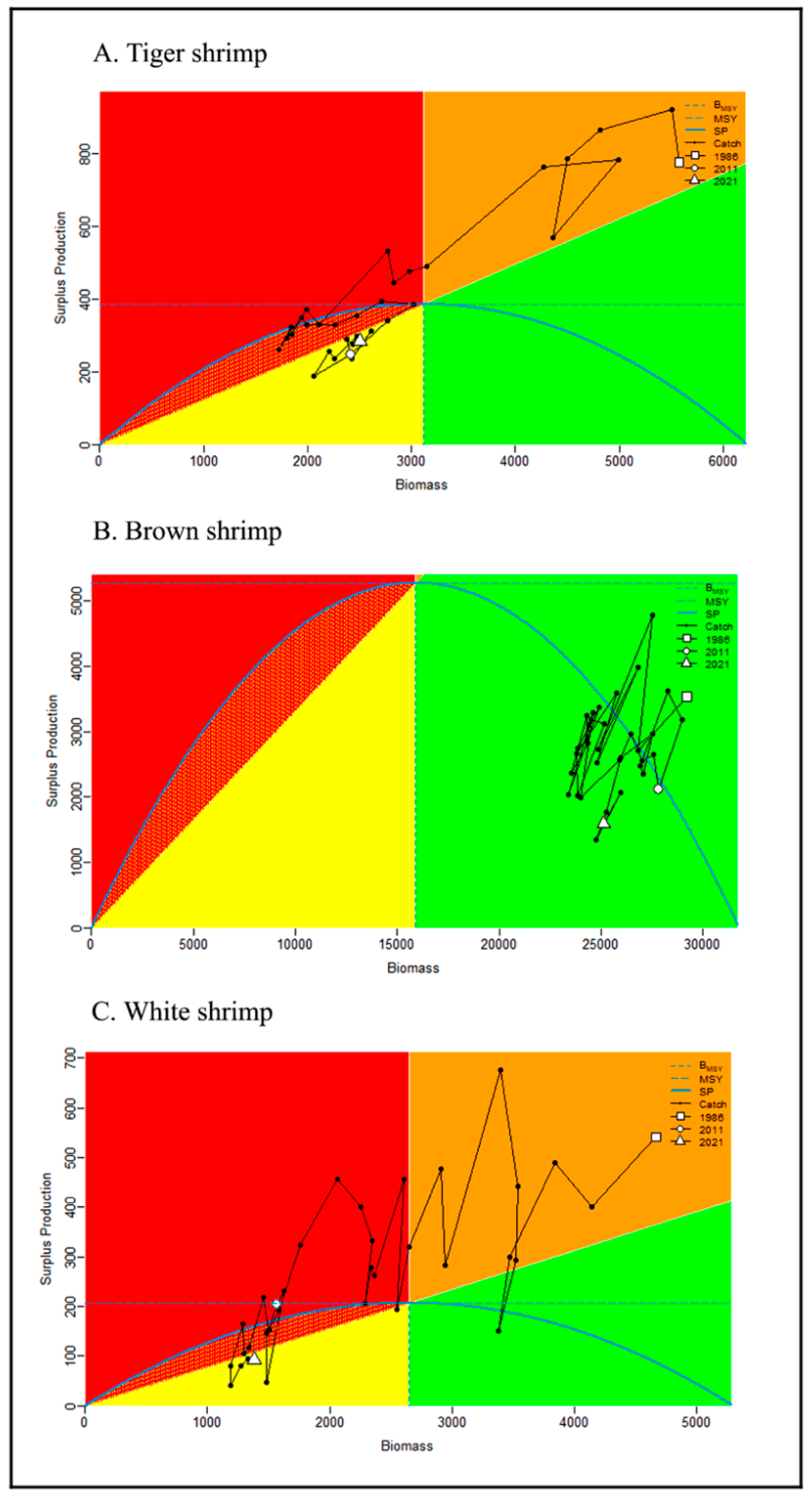
3.4. Shrimp’s Stock Analysis Based on JABBA Outputs

The model converged and fitted the biomass index quite well, capturing the main temporal trends in the observed data of three shrimp stocks (Figure 6—model fit); therefore, the assessment of JABBA is considered the most credible in the assessment of the shrimp fisheries of Bangladesh. Even though there were noticeable variations in the fitness of abundance indices (log index in Figure 6), they were within the 95% confidence interval (CI).

Overall, observed and predicted CPUE trends showed consistency in production models. There is no indication of prior misspecification in Figure 7, which shows the posteriors and predicted prior distribution for the four important model parameters (K, r, psi, and q).

Point estimates of model parameters and key quantities are shown in

Table 4. Point estimates and 95% confidence intervals (CI) of estimated parameters using the JABBA model.

Parameters	Tiger Shrimp	Brown Shrimp	White Shrimp
K (year−1)	6232.89 (4003.64–12,361.32)	31,770.30 (15,214.16–90,873.27)	5298.48 (2816.63–9344.75)
r (year−1)	0.24 (0.12–0.41)	0.66 (0.27–1.93)	0.15 (0.07–0.37)
q	0.000024 (0.000011–0.000040)	0.000018 (0.000005–0.000042)	0.000017 (0.000007–0.000043)
MSY (mt)	388.84 (275.87–552.85)	4899.24 (2791.25–23,536.08)	208.68 (128.20–301.46)
BMSY (mt)	3116.45 (2001.82–6180.66)	15,885.15 (7607.08–45,436.64)	2649.24 (1408.31–4672.38)
FMSY (year−1)	0.12 (0.06–0.20)	0.33 (0.14–0.97)	0.08 (0.03–0.18)
B/B0	0.89 (0.74–1.07)	0.91 (0.76–1.09)	0.88 (0.73–1.08)
B2021/BMSY	0.81 (0.57–1.14)	1.64 (1.09–2.01)	0.52 (0.27–1.03)
F2021/FMSY	0.92 (0.53–1.39)	0.19 (0.04–0.49)	0.87 (0.37–1.79)

and Figure 8, along with the 95% confidence intervals. The r and K parameters are estimated as 0.24 year⁻¹ and 6232.89 mt for tiger shrimp, 0.66 year⁻¹ and 31,770.30 mt for brown shrimp, and 0.15 year⁻¹ and 5298.48 mt for white shrimp. The catchability coefficient (q) is almost close among the three species. The estimated MSY values are 388.84 mt, 4899.24 mt, and 208.68 mt for the tiger, brown, and white shrimp, respectively. The B₂₀₂₁/B_MSY values (1.64) for brown shrimp are above the target reference points of 1.0, but those of the tiger and white shrimp show as 19% (0.81) and 48% (0.52) lower than the targeted. The reference point of harvest rate for brown shrimp is higher (0.33) than tiger shrimp (0.12) and white shrimp (0.08). Accordingly, the estimated F₂₀₂₁/F_MSY values (0.92, 0.19, and 0.87 for tiger, brown, and white shrimp, respectively) are smaller than 1.0, indicating a much lower fishing mortality for brown shrimp than absorbance. Both of these reference points show that the brown shrimp biomass is currently above more than 150% of the target reference point (B/B_MSY = 1), and the fishing mortality is presently 80% lower than the target reference point (F/F_MSY = 1).

The Kobe plots (Figure 9) illustrate the simultaneous development of the B/B_MSY and F/F_MSY for the tiger and white shrimps, except for the brown shrimp. The plot for tiger shrimp shows a gradual stock depletion from 1986, moving from a healthy stock with sustainable fishing pressure to a stock already depleted by over-fishing before 2010. Then, the stock slowly recovers with lower fishing pressure than F_MSY. In 2021, the stock remained in the yellow zone with more than 50% probability, where reduced fishing pressure was gradually being approached to produce maximum sustainable yield (MSY). The plot for brown shrimp showed a terrific scenario, where the stock from 1986 to 2021 always remained above B_MSY, having 100% probability in a healthy zone (green) of the Kobe plot, with a sustainable fishing pressure that was immensely lower than the F_MSY. The plot of white shrimp showed the gradual stock reduction from 1986 and moved from a healthy stock employing high fishing pressure to a stock that already been depleted by over-fishing until 2016. In 2021, the stock moved in the recovery zone with a 62% probability where stock biomass and fishing pressure are below reference points. On the other hand, the surplus production phases (Figure 10) for the three shrimp stocks indicate that surplus production is remarkably larger than the catches of the entire study period for brown shrimp. Surplus production is not significantly more significant than the catches from 2011 to the end of the study year for both tiger and white shrimps. Although, catches of the first half of the entire study years were always above surplus production for both tiger and white shrimps. Therefore, the biomass for three shrimp stocks had a high probability of increasing if the current level of fishing pressure was maintained.

4. Discussion

4.1. Stock Condition Analysis Based on LBB Approaches

Assumptions of the LBB approach, such as recruitment, growth, and mortality, should be considered. Thus, using this method should not be recommended if these assumptions are violated. The result of this method will be questioned if LF data are not representative. For reliable LF data, the LBB method can provide comparatively robust advice to the data-limited stocks [21]. In this study, the length–frequency data collections randomly covered different sizes from the catch of trawl nets throughout the year from different areas so that fish species of almost all sizes and different water areas were sampled.

LBB is a new assessment tool to assess length-based data for data-limited fishery. The Bayesian Monte Carlo Markov Chain (MCMC) approach is used in LBB to estimate all parameters. Herein, for MCMC, as the output of the Bayesian statistics, the main advantage is that the posterior inference is straightforward, which can give direct information about the parameter asked for [55,56] and calculate credible probability distributions simultaneously for multiple parameters, with model prediction as well [57]. $L_{\infty }, F/M$, $Z/K$, $F/k$, $B/B_0$, $B/B_{MSY},$ and $L_{c50}$ are some key parameters that were estimated with 95% confidence intervals, and these results could provide decisive information on the stock of interest. The calculated asymptotic length L_∞ (CL) for tiger and brown shrimps were estimated in the present study, which were higher than the estimates of a previous study by Mustafa et al. 2006 [18], where they mentioned total length (TL) of shrimp species separated by sex. In our study, we arbitrarily found conversion values from TL to CL as 3.1, 3.1, and 3.4 for tiger, brown, and white shrimps, respectively. But, white shrimp (Fenneropenaeus indicus) was not included in their study. Based on the stock status given by Palomares et al. (2018), the leading results of the LBB for industrial shrimp fisheries in Bangladesh marine waters show very interesting information, including tiger shrimp being grossly overfished, both brown shrimp and white shrimp being fully exploited but not overfished, and suggesting fairly good stock [58]. Tiger shrimp is a desired item in the export market [8], but the stock is now heavily overfished. These results are generally consistent with some previous studies on major industrial shrimp stocks [1,7,8,10], which found that the biomass of tiger shrimp population is suffering from depletion, as are other main commercial fish species, which corresponded to the lowered CPUE trend in finfish in the historical catch along Bangladesh marine waters [59].

Overfishing is a leading anthropogenic issue in marine ecosystems and has reduced biodiversity and impaired ecosystem function [60]. A study by the Food and Agricultural Organization (FAO) of the United Nations suggested that 31.4% of global fish stock is overfished, and 58.1% is fully exploited [61]. Although, this statistic came from only 20% of global catches, where less than 1% of all species have been assessed [62]. Therefore, the practical situation of worldwide stock status is likely to be even worse. The result of $L_c/L_{c\_opt}$ was less than one for tiger shrimp but not for white and brown shrimps. This result suggests the tiger shrimp stock suffers from growth overfishing [63]. Growth overfishing occurs when fish are caught before they reach their optimum size, along with plummeting fishery performances [64].

4.2. Stock Condition Analysis Based on Length-Based Indicators

We have analyzed the catch composition to determine the proportion of mature fish (P_mat), optimally sized fish (P_opt), and mega-spawners (P_mega) using the sustainability indicators proposed by Froese (2004) [37], who suggested to advise stock assessment indicators in a form that the general public could understand to tackle deliberate overfishing and to encourage the responsible use of aquatic resources. Length–frequency data make these predictions easy. To minimize growth overfishing, the catch should contain as many mature fish (P_mat) as possible and be within 10% of optimum length (L_opt) [37]. The findings of this study depict good sizes of mature individuals of tiger and white shrimps, which made up the bulk of the catch (86% and 92% of P_mat, with 63% and 74% of P_mega for tiger shrimp and white shrimp, respectively). However, it showed comparatively smaller sized brown shrimp that made up the bulk of the catch (P_mat = 35%, and P_mega = 13%). All three shrimp species had a considerably low percentage of optimum-sized individuals. While this is evidence that the stock of brown shrimp is suffering from growth overfishing, the stock of both tiger and white shrimp indicate overfishing in terms of recruitment, and the smaller genre of brown shrimp is supposed to be prone to maintain itself in a smaller-sized cluster.

The calculated value of P_mega in this study was estimated to be higher for both tiger and white shrimp, indicating continually removing the larger sizes of such species from the stock. Froese (2004) advised not catching more than 30–40% of mega-spawners [37], as the mega-spawners can intensify the recruiting success and play vital roles in the proliferation of stock biomass. Hence, the low reproductive potentials of tiger and white shrimp stocks are consistent with these higher removals of the larger individuals of such species for export and breeding purposes. The Cope and Punt decision tree based on Froese indicators estimates that both tiger and white shrimp spawning stock biomasses are below the target reference point (TRP) and limit reference point (LRP) [38]. However, the spawning stock biomass for brown shrimp is substantially higher than both the TRP and LRP. From the empirical trawl catch composition and the observation of historical catch quantity, the first author, solely responsible for looking after marine catches for more than a decade as a mid-level officer of the Marine Fisheries Office under the Department of Fisheries, Bangladesh, has observed a considerable haul of brown shrimp under the existing selective pattern of gears.

Given these observations, a medium-length limit for catches larger than the length at initial sexual maturity for all three species is reasonable to advise since the fishery will be sustained at any removal rate if juvenile shrimps are allowed to grow and reproduce at least once [37]. Therefore, the recommendations on medium-length limits and associated mesh size regulations will be reasonable management measures for the decisive authority.

4.3. Stock Condition Analysis Based on JABBA Model

This study used catch–effort data and an open source Bayesian State-Space Surplus Production Model, JABBA, to assess shrimp stock biomass and its response to the current degree of fishing efforts [39]. Maximum yearly catch limits, such as MSY and TAC, are effective instruments for managing an exploited fish stock. Combining them with length-based management indicators ensures a fishery’s sustainable stock biomass. Therefore, this study coupled length-based indicators with the JABBA model to produce catch-based reference points for developing comprehensive management recommendations for the shrimp fisheries of Bangladesh. By utilizing the entire history of catch and effort records, going back to the start of the fishery’s history will provide the most accurate assessment of the stock status. Industrial shrimp trawling beyond 40 m began in 1981 with eight shrimp trawlers, but it gained momentum in 1986 when the number of shrimp trawlers expanded to 36 [35]. Offshore fish trawling in Bangladesh was first conducted in 1972 [3]. As a result, it was considered that the historical catch data from 1986 represented almost the whole history of capture for these fisheries.

In many cases, CPUE is standardized when raw fishing efforts are associated with some factors, including fleet efficiency, species targeting, the environment, and population or fishing fleet dynamics [65,66,67]. Tiger, brown, and white shrimps are the main targeting species of shrimping vessels (MFO annual catch logs). It is a fact that these three commercially important shrimp species are usually ready to export from shrimping vessels, and this is why the prevalence of the under-reporting of shrimp catches is assumed to be low [1]. The authorities restricted shrimp trawling in 2003 by not replacing ageing shrimp trawlers with new vessels [68]. This led to a decrease in fishing pressure in the subsequent years [1], and the variations among shrimping vessels were not considerably observed due to the same shapes and trawling speeds, almost all being of an old age, and the same hauling strategies of the shrimping vessels (personal interviews with skippers during data collections). In addition, shrimping vessels can fish beyond the 40 m depth contour [31,32] in the marine waters of the Bay of Bengal, Bangladesh, where no significant environmental variations are observed. Hence, this study did not standardize the fishing efforts before fitting the CPUE in the JABBA model to consider the minimal effects of such factors on fishing efforts.

Using the Schaefer surplus production function, the JABBA model estimated total reference points for assessing shrimp stocks with a reasonable degree of fitness. Due to their high resilience, shrimp can double their population quickly [69]. The prior stock’s biomass at the inception of the study was considered to be 90% of initial biomass (assuming K = initial biomass). The output of the JABBA model in Table 4 showed that the estimated biomass in 2021 is 2524 mt, which is lower than the B_MSY of 3116 mt for tiger shrimp. The average annual catch from 1986 to 2021 is 417 mt, which is higher than the estimated MSY of 389 mt. For brown shrimp, the calculated biomass in 2021 is 26,051 mt, which is nearly double of B_MSY (15,885 mt). The average annual catch from 1986 to 2021 is 2763 mt, which is about half of the estimated MSY of 4899 mt. For white shrimp, the estimated biomass in 2021 is 1377 mt, which is lower than the B_MSY of 2649 mt. The average annual catch from 1986 to 2021 is 261 mt, which is higher than the calculated MSY of 209 mt. Fishing mortality for all three major shrimp species has decreased reasonably in the last decade, and the stock biomass of these three species is approaching the safe zone (Figure 6) because of an official decision upon shrimp trawling by not replacing old shrimp trawlers with new ones [68]. As a result, at the end of the study year, the stock’s biomass was within surplus production (Figure 7) for all three shrimp species, which indicated that the stock biomass will not be depleted further and will be capable to produce MSY if the current removal rate continues [39].

Despite the high demand and economic potential, the shrimp fishery has not been valued as such, particularly in management and research. Though there are a few studies available in national and international journals for tiger and brown shrimps [1,7,8,10,16,17], no study has been found yet that solely focuses on the assessment of white shrimp. Therefore, this would be the first study on assessing white shrimp stock also.

Table 5. The means of the estimated reference points for three major shrimp species between previous and the present study with 95% confidence intervals.

Species Name	K (mt)	r (Year−1)	MSY (mt)	BMSY (mt)	*BCurrent (mt)	FMSY (year−1)	Model Used	Reference
Penaeus monodon	4720 (3350–6650)	0.45 (0.32–0.62	527 (388–717)	2360 (1670–3320)	1250 (885–1550)	0.22 (0.16–0.31)	CMSY	[8]
	5015 (3635–5808)	-	203 (166–250)	2062 (1451–2694)	1429 (626–2458)	0.13 (0.08–0.23)	DB-SRA	[7]
	6233 (4004–12,361)	0.24 (0.12–0.41)	389 (276–553)	3116 (2002–6181)	2524	0.12 (0.06–0.20)	JABBA	Present study
Metapenaeus monoceros	10,000 (8380–12,200)	1.22 (1.03–1.45)	3090 (2920–3260)	5060 (4990–6110)	5960 (4760–6830)	0.61 (0.51–0.73)	CMSY	[10]
	35,871 (26,192–40,750)	-	1408 (1155–1715)	15,140 (10,795–19,320)	9470 (4200–17,097)	0.12 (0.07–0.20)	DB-SRA	[7]
	31,770 (15,214–90,873)	0.66 (0.27–1.93)	4899 (2791–23,536)	15,885 (7607–45,437)	26,051	0.33 (0.14–0.97)	JABBA	Present study
Fenneropenaeus indicus	5298 (2817–9345)	0.15 (0.07–0.37)	209 (128–301)	2649 (1408–4672)	1377	0.08 (0.03–0.18)	JABBA	Present study

* B_Current stands for biomass in the reference year of 2022.

showed that the present and previous study’s results vary in all parameters. Particularly for tiger shrimp, a significant variation is observed in K and r. The estimated K values by Barua et al. (2020) [8] and Alam et al. (2022) [7] were much lower than the present study. However, the 95% confidence intervals of their estimates of K overlapped with the range of this study’s estimates. The estimation of r by Barua et al. (2020) was much higher than in the present study [8]. But, other reference points related to biomass, such as MSY, B_MSY, and F_MSY of the present study, were around the results of previous studies. The estimated mean biomass for the reference year of 2021 was significantly higher than those of previous studies.

For brown shrimp, the estimates of K and r in the present study were within the results of previous studies [7,10]. The estimated MSY and mean biomass in the reference year of the present research were much higher than those of Barua (2021) and Alam et al. (2022) [7,10]. The estimated B_MSY in the present study was near to the result of Alam et al. (2022) [7], which was far higher from Barua (2021) [10]; the calculated value of F_MSY in the present study was between the result of Barua (2021) and Alam et al. (2022) [7,10]. One of the main reasons for such variations in estimated parameters using the same stock is the application of different models to assess the stock. A significant disparity has been observed in different parameter estimates of brown shrimp, especially in the MSY and the high mean biomass of the reference year (B_current). The high resilience of the brown shrimp species (population doubling time < 15 months) [69] and female spawns once every two months [70] made the vast availability of brown shrimp in the marine waters of the Bay of Bengal, Bangladesh. If we consider the empirical situation that prevailed in the present fishing fleet, then we have observed a lot of brown shrimp catches by other demersal finfish trawlers that are actually listed as shrimp catches not truly specified under brown shrimp catches in the catch log (personal observation). Therefore, the increased estimation of brown shrimp biomass elucidated by the present study is justified based on the current stock scenario. Moreover, no inclusions of shrimp trawlers in the present fishing fleet and an annual fishing ban for 87 days significantly contribute to this augmentation of brown shrimp in present years.

For white shrimp, the catch was above the MSY (209 mt) in the initial years of study. Though the catch showed fluctuations from 1990 to 2005, the catch trend has declined since 2005. The real catch was sharp, below the MSY reference point in the years from 2005 to 2021 (Figure 6). There were no changes in stock size throughout the study’s years, but it always remained in a declining state. The low-performing nature of F. indicus stock was because of the engagement of more effort than absorbance during the inception of the trawling industry; hence, there was supposed to be no space for rebuilding the stock. The poor performance of this white shrimp stock from 2005 to 2021 (Figure 9) may have resulted from the biology of this species, such as its low fecundity, less survival rate of PL (Post Larva), less spawning frequency, poor habitat interaction, poor prey–predator relationship, etc. In addition, indiscriminate killing of the PL of other shrimp species during the collection of the PL of tiger shrimp by subsistence coastal fishers for year after year has consequently driven the stock of white shrimp to a diminishing rate because the post-larvae of this species coexist with the post-larvae of tiger shrimp in a great abundance along the coastal peripheries [71].

5. Conclusions

Multi-methodological approaches provide a path forward for the better assessment of data-limited fisheries and a means to obtain a greater understanding of stock status when cautiously articulated, estimating all parameters than may be obtained from a single-assessment approach in isolation. Given the substantial economic importance and demand for shrimp fisheries both domestically and abroad, this study used a suite of different methods, including two length-based and catch-based methods, to robustly evaluate growth parameters, current stock statuses, and optimum length limits for capture. Although there is only a length-based study for assessing tiger and brown shrimps in the marine waters of Bangladesh, it is not wise to convert length into imaginary ages through length-converted catch curves for penaeid shrimps, where more than a cohort is observed, i.e., growth is seasonal. Hence, comparisons have been drawn with previous studies that assessed using catch-based approaches. In this study, both length-based and catch-based methods displayed the actual situations of the stock, e.g., the stock of brown shrimp is in a better state than those of tiger and white shrimps, except for some fluctuations in a few estimates. Hence, it is possible to draw the following conclusion from these results:

• The von Bertalanffy Growth Function (VBGF) parameters for tiger, brown, and white shrimps were L_∞ = 113.0 mm, 85.4 mm, and 76.4 mm, respectively, for carapace length;
• The relative biomass level (B/B_MSY) of the tiger shrimp was 0.43, suggesting an overfishing status, and the values of the brown and white shrimps were 0.84 and 0.96, respectively, indicating that they were fully exploited but not overfished. The estimates of L_c/L_{c_opt} were less than the unity for tiger and brown shrimps, suggesting that the stocks were suffering from growth overfishing;
• This study recommended an optimum length limit to catch from 57.0–70.0 mm for tiger shrimp, 44.0–53.0 mm for brown shrimp, and 40.0–48.0 mm for white shrimp;
• The estimated maximum sustainable yield (MSY) reference points were optimal: biomass B_MSY = 3116 mt, 15,885 mt, and 2649 mt for tiger, brown and white shrimp, respectively, and optimal harvest rate uMSY = 12%, 33%, and 8% for tiger, brown and white shrimp, respectively. The average annual catch for the last ten years was below the estimated MSY values of 389 mt, 4899 mt, and 209 mt for tiger, brown, and white shrimp, respectively;
• Brown shrimp were calculated using the JABBA model to have the highest carrying capacity (31,770 mt) and intrinsic growth rate (66%) compared to tiger and white shrimp. The ratio of fishing mortality for brown shrimp was the lowest (F/F_MSY = 0.19) among the three shrimp species. Similarly, the proportion of fishing and natural mortality calculated using the LBB model showed the lowest and prudent estimate for brown shrimp (F/M = 0.99) compared to the tiger (=2.6) and white shrimps (=1.31). Therefore, the stock of brown shrimp was concluded to be in a better state than those of the tiger and white shrimps.

References

1. Barua, S.; Magnusson, A.; Humayun, N.M. Assessment of offshore shrimp stocks of Bangladesh based on commercial shrimp trawl logbook data. Indian J. Fish. 2018, 65, 1–6. [Google Scholar] [CrossRef]
2. DoF. National Fish Week 2022 Compendium (in Bangla); Department of Fisheries, Ministry of Fisheries and Livestock: Dhaka, Bangladesh, 2022; 170p. Available online: www.fisheries.gov.bd (accessed on 20 March 2023).
3. Rahman, A.K.A.; Khan, M.G.; Chowdhury, Z.A.; Hussain, M.M. Economically Important Marine Fishes and Shellfishes of Bangladesh; Department of Fisheries: Dhaka, Bangladesh, 1995. [Google Scholar]
4. Penn, J.W. The Current Status of Off Shore Marine Fish Stocks in Bangladesh Waters with Special Reference to Penaeid Shrimp Stocks; FAO: Rome, Italy, 1982; 47p. [Google Scholar]
5. Fanning, P.; Chowdhury, S.R.; Uddin, M.S.; Al-Mamun, M.A. Marine Fisheries Survey Reports and Stock Assessment 2019; Bangladesh Marine Fisheries Capacity Building Project, Department of Fisheries, Ministry of Fisheries and Livestock: Dhaka, Bangladesh, 2019. Available online: http://mfsmu.fisheries.gov.bd/site/download/03cb42dc-8a4f-4dd3-a08943e5f5bcf61b (accessed on 20 March 2023).
6. Lamboeuf, M. Bangladesh Demersal Fish Resources of the Continental Shelf; R/V Anusandhani Trawling Survey Results (September 1984–June 1986); FAO: Rome, Italy, 1987; 26p. [Google Scholar]
7. Alam, M.S.; Liu, Q.; Schneider, P.; Mozumder, M.M.H.; Uddin, M.M.; Monwar, M.M.; Hoque, M.E.; Barua, S. Stock Assessment and Rebuilding of Two Major Shrimp Fisheries (Penaeus monodon and Metapenaeus monoceros) from the Industrial Fishing Zone of Bangladesh. J. Mar. Sci. Eng. 2022, 10, 201. [Google Scholar] [CrossRef]
8. Barua, S.; Al Mamun, M.A.; Nazrul, K.M.S.; Mamun, A.; Das, J. Maximum sustainable yield estimate for Tiger shrimp, Penaeus monodon off Bangladesh coast using trawl catch log. Bangladesh Marit. J. 2020, 4, 135–144. [Google Scholar]
9. FRSS. Fisheries Resources Survey System: Fisheries Statistical Report of Bangladesh; Department of Fisheries (DoF), Ministry of Fisheries and Livestock (MoFL): Dhaka, Bangladesh, 2022; Volume 31, pp. 1–57. [Google Scholar]
10. Barua, S. Maximum sustainable yield estimate for Brown shrimp, Metapenaeus monoceros (Fabricius 1798) in marine waters of Bangladesh using trawl catch log. Indian J. Geo-Mar. Sci. 2021, 50, 258–261. [Google Scholar]
11. West, W.Q.B. Fishery Resources of the Upper Bay of Bengal. Indian Ocean Programme, Indian Ocean Fisheries Commission, IOFC/DEV/73/28; FAO: Rome, Italy, 1973; 44p. [Google Scholar]
12. Rashid, M.H. Mitsui Taiyo shrimp survey 1976-77 by the survey research vessels M. V. Santa Monica and M. V. Orion 8 in the marine waters of Bangladesh. Mar. Fish. Bull. 1983, 2, 23. [Google Scholar]
13. White, T.F.; Khan, M.G. The marine resources of Bangladesh and their potential for commercial development. In Proceedings of the National Seminar on Fisheries Development in Bangladesh, Dhaka, Bangladesh, 1–4 January 1985; pp. 1–4. [Google Scholar]
14. Hilborn, R.; Walters, C.J. Quantitative Fisheries Stock Assessment, Choices, Dynamics and Uncertainty; Chapman and Hall: New York, NY, USA, 1992. [Google Scholar]
15. Quinn, T.J.; Deriso, R.B. Quantitative Fish Dynamics; Oxford University Press: New York, NY, USA, 1999. [Google Scholar]
16. Khan, M.S.; Hoque, M.S. Bioeconomics modelling: Bangladesh shrimp fishery. In International Seminar in Malaysia; Malaysia Construction Industry Development Board: Kuala Lumpur, Malaysia, 2000. [Google Scholar]
17. Kar, T.K.; Chakraborty, K. A bioeconomic assessment of the Bangladesh shrimp fishery. World J. Model. Simul. 2011, 7, 58–69. [Google Scholar]
18. Mustafa, M.G.; Ali, M.S.; Azadi, M.A. Some aspect of population dynamics of three penaeid shrimps (Penaeus monodon, Penaeus semisulcatus and Metapenaeus monoceros) from the Bay of Bengal, Bangladesh. Chittagong Univ. J. Sci. 2006, 30, 97–102. [Google Scholar]
19. Mildenberger, T.K.; Taylor, M.H.; Wolff, M. TropFishR: An R package for fisheries analysis with length-frequency data. Methods Ecol. Evol. 2017, 8, 1520–1527. [Google Scholar] [CrossRef]
20. Hordyk, A.; Ono, K.; Sainsbury, K.; Loneragan, N.; Prince, J. Some explorations of the life history ratios to describe length composition, spawning-per-recruit, and the spawning potential ratio. ICES J. Mar. Sci. 2015, 72, 204–216. [Google Scholar] [CrossRef]
21. Froese, R.; Winker, H.; Coro, G.; Demirel, N.; Tsikliras, A.C.; Dimarchopoulou, D.; Scarcella, G.; Probst, W.N.; Dureuil, M.; Pauly, D. A new approach for estimating stock status from length frequency data. ICES J. Mar. Sci. 2018, 75, 2004–2015. [Google Scholar] [CrossRef]
22. Sparre, P. Can we use traditional length-based fish stock assessment when growth is seasonal? Fishbyte 1990, 8, 29–32. [Google Scholar]
23. Smith, D.; Punt, A.; Dowling, N.; Smith, A.; Tuck, G.; Knuckey, I. Reconciling approaches to the assessment and management of data-poor species and fisheries with Australia’s harvest strategy policy. Mar. Coast. Fish. Dyn. Manag. Ecosyst. Sci. 2009, 1, 244–254. [Google Scholar] [CrossRef]
24. Agnew, D.J.; Gutiérrez, N.L.; Butterworth, D.S. Fish catch data: Less than what meets the eye. Mar. Policy 2013, 42, 268–269. [Google Scholar] [CrossRef]
25. Branch, T.A.; Jensen, O.P.; Ricard, D.; Ye, Y.; Hilborn, R. Contrasting Global Trends in Marine Fishery Status Obtained from Catches and from Stock Assessments. Conserv. Biol. 2011, 25, 777–786. [Google Scholar] [CrossRef] [PubMed]
26. Prager, M.H. ASPIC: A Surplus-Production Model Incorporating Covariates. Coll. Vol. Sci. Pap. Int. Comm. Conserv. Atl. Tunas 1992, 28, 218–229. [Google Scholar]
27. Martell, S.; Froese, R. A simple method for estimating MSY from catch and resilience. Fish Fish. 2013, 14, 504–514. [Google Scholar] [CrossRef]
28. Rosenberg, A.A.; Fogarty, M.J.; Cooper, A.B.; Dickey-Collas, M.; Fulton, E.A.; Gutiérrez, N.L.; Hyde, K.J.W.; Kleisner, K.M.; Kristiansen, T.; Longo, C.; et al. Developing New Approaches to Global Stock Status Assessment and Fishery Production Potential of the Seas; FAO Fisheries and Aquaculture Circular No. 1086; FAO: Rome, Italy, 2014; 175p. [Google Scholar]
29. Raza, H.; Liu, Q.; Alam, M.S.; Han, Y. Length based stock assessment of five fish species from the marine water of Pakistan. Sustainability 2022, 14, 1587. [Google Scholar] [CrossRef]
30. Barua, S.; Thordarson, G.; Jonsdottir, I.G. Comparison of catch and survey data for assessing northern shrimp (Pandalus borealis) from Arnarfjordur (NW-Iceland) using a stock production model. Turk. J. Fish. Aquat. Sci. 2018, 18, 359–366. [Google Scholar] [CrossRef]
31. MFA. 2020. Marine Fisheries Act 2020. Ministry of Fisheries and Livestock, SRO 211-AIN/2019, 24 June 2019. Available online: http://bdlaws.minlaw.gov.bd/act-1347.html (accessed on 10 June 2022).
32. MFO. Marine Fisheries Ordinance 1983 (Bangladesh). 1983. Available online: http://www.fisheries.gov.bd/sites/default/files (accessed on 10 June 2022).
33. IOTC. IOTC National Report 2020 (Bangladesh part). 2020; National Report of Bangladesh for IOTC; IOTC: Dhaka, Bangladesh, 2020. [Google Scholar]
34. Barua, S.; Karim, E.; Humayun, N.M. Present status and species composition of commercially important finfish in landed trawl catch from Bangladesh marine waters. J. Pure Appl. Zool. 2014, 2, 150–159. [Google Scholar]
35. Islam, M.S. Perspectives of the coastal and marine fisheries of the Bay of Bengal, Bangladesh. Ocean Coast. Manag. 2003, 46, 763–796. [Google Scholar] [CrossRef]
36. Barua, S.; Liu, Q.; Alam, M.S.; Schneider, P.; Mozumder, M.M.H.; Rouf, M.A. Population dynamics and stock assessment of two major eels (Muraenesox bagio and Congresox talabonoides) from the marine waters of Bangladesh. Front. Mar. Sci. 2023, 10, 1134343. [Google Scholar] [CrossRef]
37. Froese, R. Keep it simple: Three indicators to deal with overfishing. Fish Fish. 2004, 5, 86–91. [Google Scholar] [CrossRef]
38. Cope, J.M.; Punt, A.E. Length-based reference points for data-limited situations: Applications and restrictions. Mar. Coast. Fish. Dyn. Manag. Ecosyst. Sci. 2009, 1, 169–186. [Google Scholar] [CrossRef]
39. Winker, H.; Carvalho, F.; Kapur, M. JABBA: Just another bayesian biomass assessment. Fish. Res. 2018, 204, 275–288. [Google Scholar] [CrossRef]
40. Froese, R.; Winker, H.; Coro, G.; Demirel, N.; Tsikliras, A.C.; Dimarchopoulou, D.; Scarcella, G.; Probst, W.N.; Dureuil, M.; Pauly, D. A Simple User Guide for LBB (LBB_33a.R). 2019. Available online: http://oceanrep.geomar.de/44832/ (accessed on 11 October 2020).
41. Von Bertalanffy, L. A quantitative theory of organic growth (inquiries on growth laws. ii). Hum. Biol. 1938, 10, 181–213. [Google Scholar]
42. Sparre, P.; Venema, S.C. Introduction to Tropical Fish Stock Assessment—Part 1: Manual. FAO Fish. Tech. Pap. 1998, 306, 1407. [Google Scholar]
43. Holt, S.J. The evaluation of fisheries resources by the dynamic analysis of stocks, and notes on the time factors involved. In International Commission for the Northwest Atlantic Fisheries; ICNAF Special Publication: Vancouver, BC, Canada, 1958; pp. 77–95. [Google Scholar]
44. Beverton, R.J.H.; Holt, S.J. On the Dynamics of Exploited Fish Populations; Ministry of Agriculture, Fisheries and Food: London, UK, 1957. [Google Scholar]
45. Beverton, R.J.H.; Holt, S.J. Manual of methods for fish stock assessment, Part II—Tables of yield functions. In FAO Fisheries Technical Paper No. 38; FAO: Rome, Italy, 1966; p. 10. [Google Scholar]
46. Amorim, P.; Sousa, P.; Jardim, E.; Menezes, G.M. Sustainability status of data-limited fisheries: Global challenges for snapper and grouper. Front. Mar. Sci. 2019, 6, 654. [Google Scholar] [CrossRef]
47. Pella, J.J.; Tomlinson, P.K. A generalized stock production model. InterAmerican Trop. Tuna Comm. Bull. 1969, 13, 421–458. [Google Scholar]
48. Fox, W.W., Jr. An exponential surplus-yield model for optimizing exploited fish populations. Trans. Am. Fish. Soc. 1970, 99, 80–88. [Google Scholar] [CrossRef]
49. Thorson, J.T.; Cope, J.M.; Branch, T.A.; Jensen, O.P. Spawning biomass reference points for exploited marine fishes, incorporating taxonomic and body size information. Can. J. Fish. Aquat. Sci. 2012, 69, 1556–1568. [Google Scholar] [CrossRef]
50. Wang, S.P.; Maunder, M.N.; Aires-da-Silva, A. Selectivity’s distortion of the production function and its influence on management advice from surplus production models. Fish. Res. 2014, 158, 181–193. [Google Scholar] [CrossRef]
51. Barrowman, N.J.; Myers, R.A. Still more spawner–recruitment curves: The hockey stick and its generalizations. Can. J. Fish. Aquat. Sci. 2000, 57, 665–676. [Google Scholar] [CrossRef]
52. ICCAT. Report of the 2017 ICCAT Atlantic Swordfish Stock Assessment Session; Retrieved from Collection of Volume Scientific Papers; ICCAT: Madrid, Spain; Volume 74, pp. 841–967.
53. Meyer, R.; Millar, R.B. BUGS in Bayesian stock assessments. Can. J. Fish. Aquat. Sci. 1999, 56, 1078–1086. [Google Scholar] [CrossRef]
54. Maunder, M.N.; Piner, K.R. Dealing with data conflicts in statistical inference of population assessment models that integrate information from multiple diverse data sets. Fish. Res. 2017, 192, 16–27. [Google Scholar] [CrossRef]
55. Cowles, M.K.; Carlin, B.P. Markov chain Monte Carlo convergence diagnostics: A comparative review. J. Am. Stat. Assoc. 1996, 91, 883–904. [Google Scholar] [CrossRef]
56. O’Hara, R.B.; Sillanpää, M.J. A review of Bayesian variable selection methods: What, how and which. Bayesian Anal. 2009, 4, 85–117. [Google Scholar] [CrossRef]
57. Haddon, M. Modelling and Quantitative Methods in Fisheries, 2nd ed.; Chapman and Hall: New York, NY, USA, 2010. [Google Scholar]
58. Palomares, M.L.D.; Froese, R.; Derrick, B.; Nöel, S.-L.; Tsui, G.; Woroniak, J.; Pauly, D. A preliminary global assessment of the status of exploited marine fish and invertebrate populations. In A Report Prepared by the Sea Around Us for OCEANA; OCEANA: Washington, DC, USA, 2018; p. 64. [Google Scholar]
59. Barua, S. Maximum Sustainable Yield (MSY) estimates for industrial finfish fishery in marine waters of Bangladesh using trawl catch log. Bang. J. Fish. 2019, 31, 313–324. [Google Scholar]
60. Worm, B.; Hilborn, R.; Baum, J.K.; Branch, T.A.; Collie, J.S.; Costello, C.; Fogarty, M.J.; Fulton, E.A.; Hutchings, J.A.; Jennings, S.; et al. Rebuilding global fisheries. Science 2009, 325, 578–585. [Google Scholar] [CrossRef]
61. FAO; Garcia, S.M.; Ye, Y.; Rice, J.; Charles, A. Rebuilding of marine fisheries Part 1: Global review. FAO Fish. Aquac. Tech. Pap. 2018, 630, I-274. [Google Scholar]
62. Costello, C.; Ovando, D.; Hilborn, R.; Gaines, S.D.; Deschenes, O.; Lester, S.E. Status and solutions for the world’s unassessed fisheries. Science 2012, 338, 517–520. [Google Scholar] [CrossRef]
63. Liang, C.; Xian, W.; Liu, S.; Pauly, D. Assessments of 14 exploited fish and Invertebrate stocks in Chinese waters using the LBB method. Front. Mar. Sci. 2020, 7, 314. [Google Scholar] [CrossRef]
64. Nadon, M.O.; Ault, J.S.; Williams, I.D.; Smith, S.G.; DiNardo, G.T. Length-based assessment of coral reef fish populations in the main and northwestern Hawaiian Islands. PLoS ONE 2015, 10, e0133960. [Google Scholar] [CrossRef] [PubMed]
65. Hampton, J.; Sibert, J.R.; Kleiber, P.; Maunder, M.N.; Harley, S.J. Changes in abundance of large pelagic predators in the Pacific Ocean. Nature 2005, 434, E2–E3. [Google Scholar] [PubMed]
66. Hinton, M.G.; Maunder, M.N. Methods for standardizing CPUE and how to select among them. Col. Vol. Sci. Pap. ICCAT 2004, 56, 169–177. [Google Scholar]
67. Branch, T.A.; Hilborn, R.; Haynie, A.C.; Fay, G.; Flynn, L.; Griffiths, J.; Marshall, K.N.; Randall, J.K.; Scheuerell, J.M.; Ward, E.J.; et al. Fleet dynamics and fishermen behavior: Lessons for fisheries managers. Can. J. Fish. Aquat. Sci. 2006, 63, 1647–1668. [Google Scholar] [CrossRef]
68. MoFL. Circular No. 160; Ministry of Fisheries and Livestock, Bangladesh Secretariat: Dhaka, Bangladesh, 2003. [Google Scholar]
69. Froese, R.; Pauly, D. (Eds.) FishBase 2000: Concepts, Design, and Data Sources; WorldFish: Penang, Malaysia, 2000; 344p. [Google Scholar]
70. Rao, G.S. Studies on the reproductive biology of the brown prawn Metapenaeus monoceros (Fabricius, 1798) along the Kakinada coast. Indian J. Fish. 1989, 36, 107–123. [Google Scholar]
71. Khan, R.N.; Aravindan, N.; Kalavati, C. Distribution of two post larvae species of commercial prawns (Fenneropenaeus indicus and Penaeus monodon) in a coastal tropical estuary. J. Aquat. Sci. 2001, 16, 99–104. [Google Scholar] [CrossRef]
Figure 1. Map of the Bay of Bengal Bangladesh marine waters showing industrial fishing zone (beyond 40 m depth colored by deep sky) and the location of sample unloading (red circle) [7,36].
Sustainability 15 12835 g001
Figure 2. Data collection on shrimps. (A) Tiger shrimp, (B) Brown shrimp, and (C) White shrimp from industrial shrimping vessels at sea.
Sustainability 15 12835 g002
Figure 3. The bar chart illustrates the length–frequency distributions of (A) tiger shrimp, (B) brown shrimp, and (C) white shrimp based on month-wise data collection from July 2021 to May 2022.
Sustainability 15 12835 g003
Figure 4. LBB plots for (A) tiger shrimp, (B) brown shrimp, and (C) white shrimp from the Bay of Bengal, Bangladesh. The left curves show the fits of the model to the length data, and the right curves are the predictions of the LBB analysis, where Lc is the length of 50% individuals captured by the gear, Linf is the asymptotic length, and Lopt is the length where the maximum biomass of the unexploited stock is obtained.
Sustainability 15 12835 g004
Figure 5. Length frequency distributions of the tiger shrimp (A), brown shrimp (B), and white shrimp (C) show the L, Lopt, and (0.9 Lopt 1.1Lopt) for the grey area.
Sustainability 15 12835 g005
Figure 6. Observed and expected index fit to the CPUE (left) and residuals (right) used for tuning the JABBA model for three major shrimp species. The solid lines in the figures are the model’s predicted values, and the circles are observed data values. Shading areas represent the estimated 95% confidence intervals around the predicted values.
Sustainability 15 12835 g006
Figure 7. Prior and posterior distributions of four key model parameters (K, r, psi, and q) for three major shrimp species. Posteriors distributions are plotted using generic kernel densities.
Sustainability 15 12835 g007
Figure 8. Estimated biomass trajectories from the model fitted to the entire time series of 1986–2021 for the three studied shrimp species. Grey-shaded areas denote 95% confidence intervals.
Sustainability 15 12835 g008
Figure 9. Kobe phase plot showing the estimated trajectories (1986–2021) of B/BMSY and F/FMSY for tiger shrimp (A), brown shrimp (B), and white shrimp (C). Different grey-shaded areas denote the terminal assessment year’s 50%, 80%, and 95% confidence intervals. The probability of terminal year points falling within each quadrant is indicated in the figure’s legend.
Sustainability 15 12835 g009
Figure 10. JABBA SP-phase plot showing estimated surplus production curves and catch/biomass trajectories (1986–2021) as a function of biomass for three major shrimp species. MSY estimates are illustrated with 95% CIs (grey-shaded area).
Sustainability 15 12835 g010