


An Automated Data-Driven Irrigation Scheduling Approach Using Model Simulated Soil Moisture and Evapotranspiration


Abstract
:1. Introduction
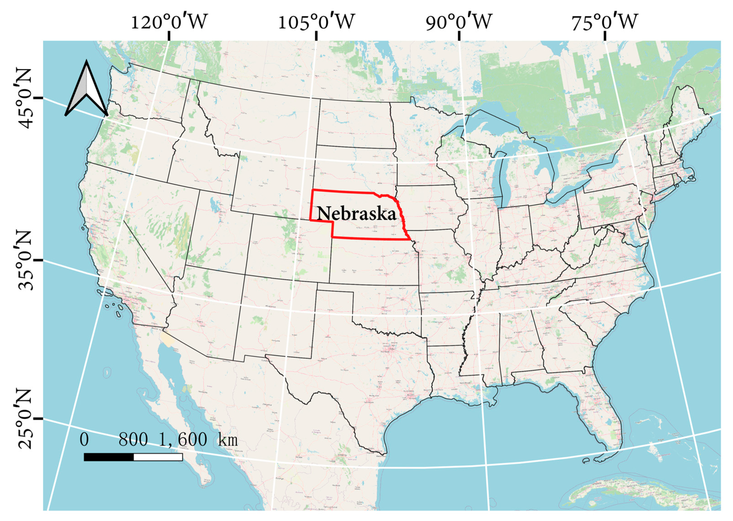
2. Study Area and Materials
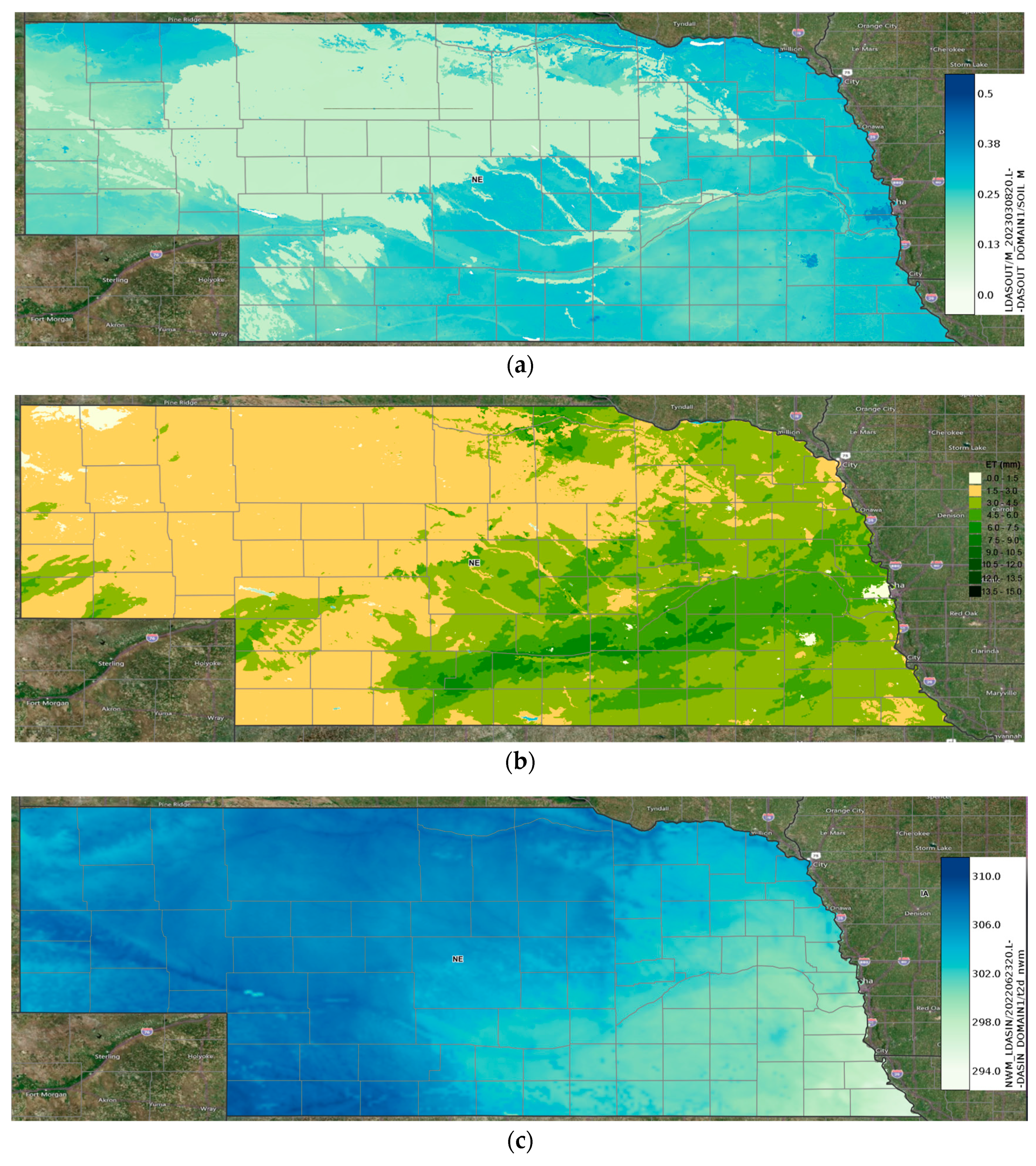
2.1. Soil Moisture and ET Map
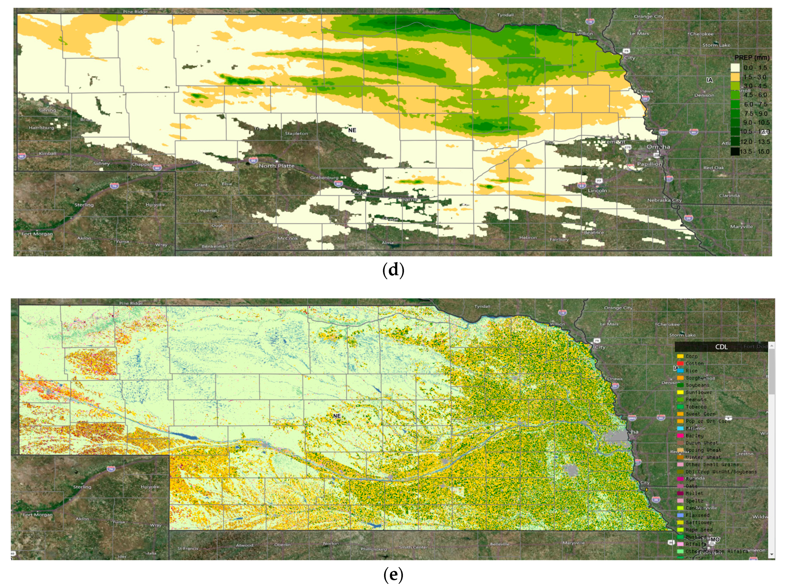
2.2. Meteorological Forcing Data
2.3. Crop Types and Soil Properties
3. Automation of the Irrigation Scheduling: The Methodology
4. Results and Discussion
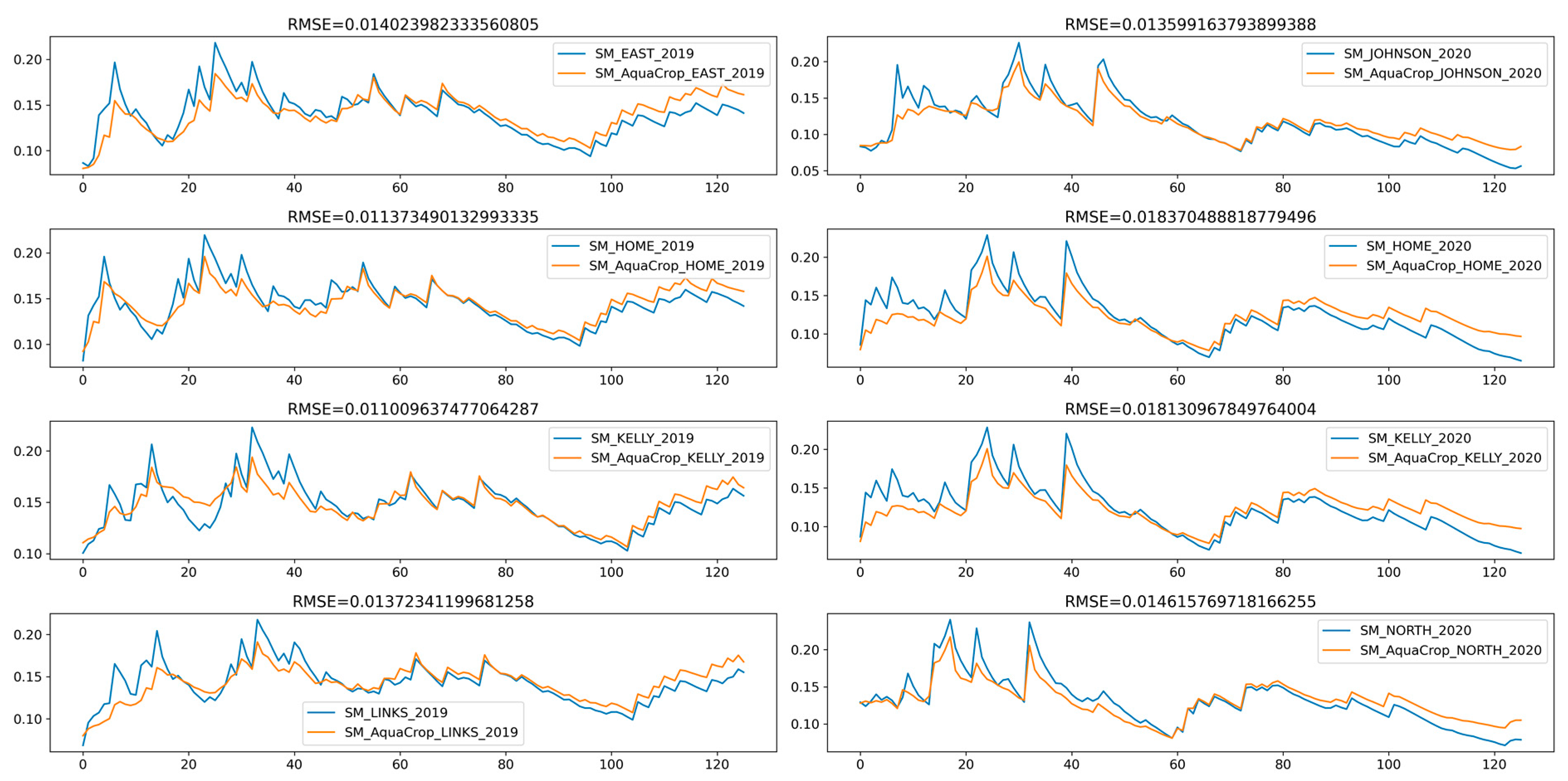
4.1. Validation of AquaCrop
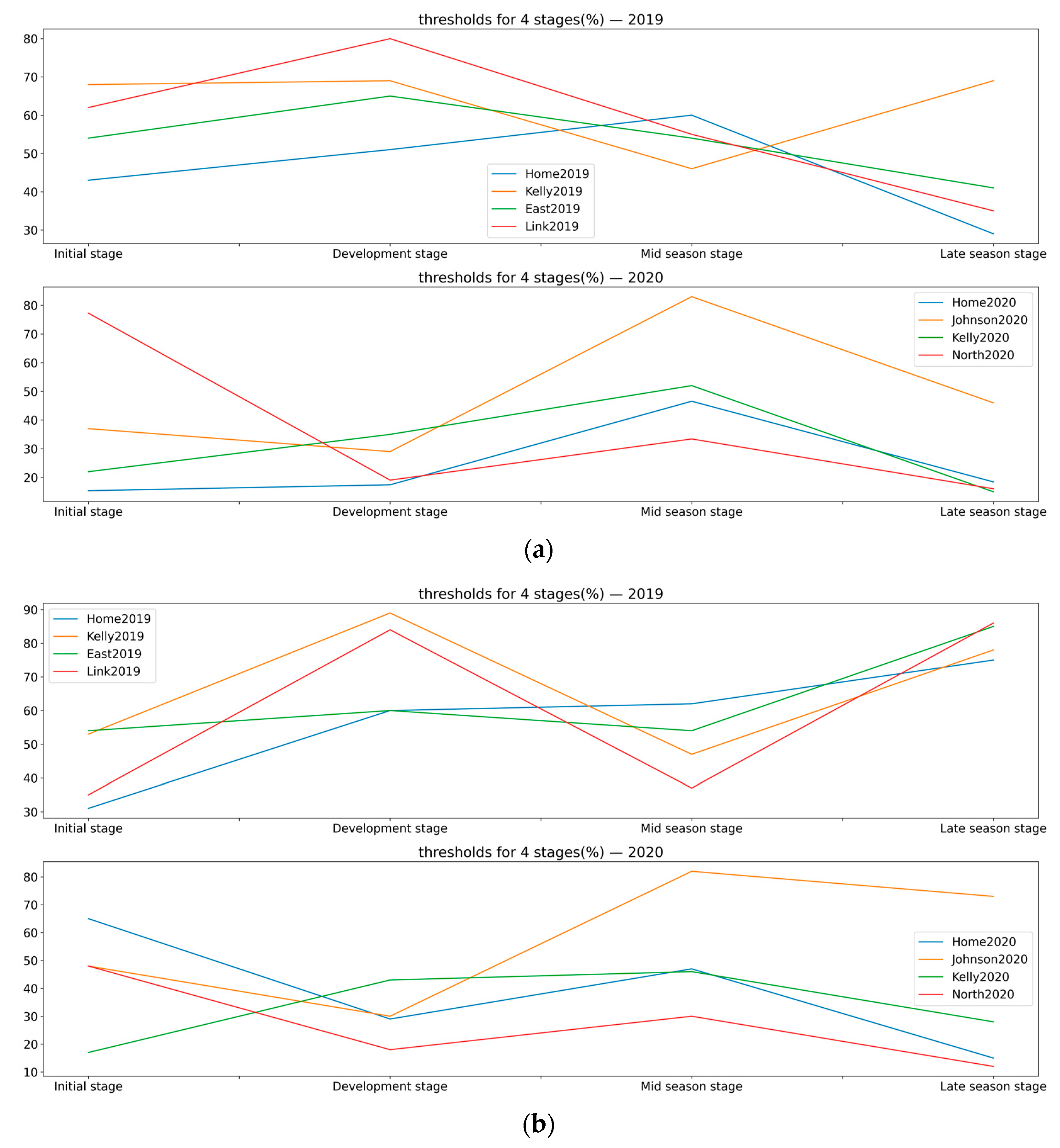
4.2. Threshold-Based Irrigation Scheduling
4.3. Irrigation Scheduling Integrating Short-Term Rainfall Forecasts
4.4. Future Work
5. Conclusions
Author Contributions
Funding
Institutional Review Board Statement
Informed Consent Statement
Data Availability Statement
Conflicts of Interest
References
- World Bank. World Bank Open Data; The World Bank Group: Washington, DC, USA, 2022. [Google Scholar]
- Walker, W.R. Guidelines for Designing and Evaluating Surface Irrigation Systems; FAO Irrigation and Drainage Paper 45; FAO: Rome, Italy, 1989. [Google Scholar]
- Dieter, C.A. Water Availability and Use Science Program: Estimated USE OF WAter in the United States in 2015; Geological Survey: Asheville, NC, USA, 2018. [Google Scholar]
- Rashad, M.; Hafez, M.; Popov, A.I.; Gaber, H. Toward sustainable agriculture using extracts of natural materials for transferring organic wastes to environmental-friendly ameliorants in Egypt. Int. J. Environ. Sci. Technol. 2023, 20, 7417–7432. [Google Scholar] [CrossRef]
- Rashad, M.; Kenawy, E.-R.; Hosny, A.; Hafez, M.; Elbana, M. An environmental friendly superabsorbent composite based on rice husk as soil amendment to improve plant growth and water productivity under deficit irrigation conditions. J. Plant Nutr. 2021, 44, 1010–1022. [Google Scholar] [CrossRef]
- Vellidis, G.; Liakos, V.; Perry, C.; Porter, W.; Tucker, M.; Boyd, S.; Huffman, M.; Robertson, B. Irrigation scheduling for cotton using soil moisture sensors, smartphone apps, and traditional methods. In Proceedings of the 2016 Beltwide Cotton Conference, New Orleans, LA, USA, 5–7 January 2016. [Google Scholar]
- Li, F.; Yu, D.; Zhao, Y. Irrigation scheduling optimization for cotton based on the AquaCrop model. Water Resour. Manag. 2019, 33, 39–55. [Google Scholar] [CrossRef]
- Viani, F. Experimental validation of a wireless system for the irrigation management in smart farming applications. Microw. Opt. Technol. Lett. 2016, 58, 2186–2189. [Google Scholar] [CrossRef]
- USDA. 2018 Irrigation and Water Management Survey; USDA-NASS: Washington, DC, USA, 2019.
- Zhao, H.; Di, L.; Sun, Z.; Hao, P.; Yu, E.; Zhang, C.; Lin, L. Impacts of Soil Moisture on Crop Health: A Remote Sensing Perspective. In Proceedings of the 2021 9th International Conference on Agro-Geoinformatics (Agro-Geoinformatics), Shenzhen, China, 26–29 July 2021; pp. 1–4. [Google Scholar]
- Chen, F.; Manning, K.W.; LeMone, M.A.; Trier, S.B.; Alfieri, J.G.; Roberts, R.; Tewari, M.; Niyogi, D.; Horst, T.W.; Oncley, S.P. Description and evaluation of the characteristics of the NCAR high-resolution land data assimilation system. J. Appl. Meteorol. Climatol. 2007, 46, 694–713. [Google Scholar]
- Myers, W.; Chen, F.; Block, J.; Meteorlogix, D.; Burnsville, M. Application of atmospheric and land data assimilation systems to an agricultural decision support system. In Proceedings of the 2007 AMS Conference on Agriculture and Forestry, Orlando, FL, USA, 27–29 July 2008. [Google Scholar]
- Zhao, H.; Di, L.; Sun, Z. WaterSmart-GIS: A Web Application of a Data Assimilation Model to Support Irrigation Research and Decision Making. ISPRS Int. J. Geo-Inf. 2022, 11, 271. [Google Scholar] [CrossRef]
- USDA National Agricultural Statistics Service. 2017 Census of Agriculture; USDA-NASS: Washington, DC, USA, 2017.
- Niu, G.Y.; Yang, Z.L.; Mitchell, K.E.; Chen, F.; Ek, M.B.; Barlage, M.; Kumar, A.; Manning, K.; Niyogi, D.; Rosero, E. The community Noah land surface model with multiparameterization options (Noah-MP): 1. Model description and evaluation with local-scale measurements. J. Geophys. Res. Atmos. 2011, 116, D12. [Google Scholar] [CrossRef]
- Cosgrove, B.; Gochis, D.; Clark, E.P.; Cui, Z.; Dugger, A.L.; Feng, X.; Karsten, L.R.; Khan, S.; Kitzmiller, D.; Lee, H.S.; et al. An Overview of the National Weather Service National Water Model. In Proceedings of the AGU Fall Meeting Abstracts, San Francisco, CA, USA, 12–16 December 2016; 2016; p. H42B-05. [Google Scholar]
- Zhao, H.; Di, L.; Sun, Z.; Yu, E.; Zhang, C.; Lin, L. Validation and Calibration of HRLDAS Soil Moisture Products in Nebraska. In Proceedings of the 2022 10th International Conference on Agro-geoinformatics (Agro-Geoinformatics), Quebec City, QC, Canada, 11–14 July 2022; pp. 1–4. [Google Scholar]
- NCEP Global Forecast System (GFS) Analyses and Forecasts; National Center for Atmospheric Research, Computational and Information Systems Laboratory: Boulder, CO, USA, 2007. [CrossRef]
- Boryan, C.; Yang, Z.; Mueller, R.; Craig, M. Monitoring US agriculture: The US department of agriculture, national agricultural statistics service, cropland data layer program. Geocarto Int. 2011, 26, 341–358. [Google Scholar] [CrossRef]
- Lark, T.J.; Schelly, I.H.; Gibbs, H.K. Accuracy, bias, and improvements in mapping crops and cropland across the United States using the USDA Cropland Data Layer. Remote Sens. 2021, 13, 968. [Google Scholar] [CrossRef]
- Lin, C.; Zhong, L.; Song, X.-P.; Dong, J.; Lobell, D.B.; Jin, Z. Early-and in-season crop type mapping without current-year ground truth: Generating labels from historical information via a topology-based approach. Remote Sens. Environ. 2022, 274, 112994. [Google Scholar] [CrossRef]
- Walkinshaw, M.; O’Geen, A.T.; Beaudette, D.E. Soil Properties; California Soil Resource Lab: Davis, CA, USA, 2022; Available online: https://casoilresource.lawr.ucdavis.edu/soil-properties/ (accessed on 13 July 2023).
- Grabow, G.; Ghali, I.; Huffman, R.; Miller, G.; Bowman, D.; Vasanth, A. Water application efficiency and adequacy of ET-based and soil moisture–based irrigation controllers for turfgrass irrigation. J. Irrig. Drain. Eng. 2013, 139, 113–123. [Google Scholar] [CrossRef]
- Qin, A.; Ning, D.; Liu, Z.; Li, S.; Zhao, B.; Duan, A. Determining threshold values for a crop water stress index-based center pivot irrigation with optimum grain yield. Agriculture 2021, 11, 958. [Google Scholar] [CrossRef]
- Allen, R.G.; Pereira, L.S.; Raes, D.; Smith, M. Crop evapotranspiration-Guidelines for computing crop water requirements-FAO Irrigation and drainage paper 56. Fao Rome 1998, 300, D05109. [Google Scholar]
- McMaster, G.S.; Wilhelm, W. Growing degree-days: One equation, two interpretations. Agric. For. Meteorol. 1997, 87, 291–300. [Google Scholar] [CrossRef]
- Miller, P.; Lanier, W.; Brandt, S. Using growing degree days to predict plant stages. Ag/Ext. Commun. Coord. Commun. Serv. Mont. State Univ.-Bozeman Bozeman MO 2001, 59717, 994–2721. [Google Scholar]
- Ahmad, L.; Habib Kanth, R.; Parvaze, S.; Sheraz Mahdi, S.; Ahmad, L.; Habib Kanth, R.; Parvaze, S.; Sheraz Mahdi, S. Growing Degree Days to Forecast Crop Stages; Springer: Berlin/Heidelberg, Germany, 2017. [Google Scholar]
- Steduto, P.; Hsiao, T.C.; Raes, D.; Fereres, E. AquaCrop—The FAO crop model to simulate yield response to water: I. Concepts and underlying principles. Agron. J. 2009, 101, 426–437. [Google Scholar] [CrossRef]
- Raes, D.; Steduto, P.; Hsiao, T.C.; Fereres, E. AquaCrop—The FAO crop model to simulate yield response to water: II. Main algorithms and software description. Agron. J. 2009, 101, 438–447. [Google Scholar] [CrossRef]
- Sandhu, R.; Irmak, S. Performance of AquaCrop model in simulating maize growth, yield, and evapotranspiration under rainfed, limited and full irrigation. Agric. Water Manag. 2019, 223, 105687. [Google Scholar] [CrossRef]
- Aziz, M.; Rizvi, S.A.; Sultan, M.; Bazmi, M.S.A.; Shamshiri, R.R.; Ibrahim, S.M.; Imran, M.A. Simulating Cotton Growth and Productivity Using AquaCrop Model under Deficit Irrigation in a Semi-Arid Climate. Agriculture 2022, 12, 242. [Google Scholar] [CrossRef]
- Lu, Y.; Chibarabada, T.P.; McCabe, M.F.; De Lannoy, G.J.; Sheffield, J. Global sensitivity analysis of crop yield and transpiration from the FAO-AquaCrop model for dryland environments. Field Crops Res. 2021, 269, 108182. [Google Scholar] [CrossRef]
- Guo, D.; Zhao, R.; Xing, X.; Ma, X. Global sensitivity and uncertainty analysis of the AquaCrop model for maize under different irrigation and fertilizer management conditions. Arch. Agron. Soil Sci. 2020, 66, 1115–1133. [Google Scholar] [CrossRef]
- Nelder, J.A.; Mead, R. A simplex method for function minimization. Comput. J. 1965, 7, 308–313. [Google Scholar] [CrossRef]
- Gao, F.; Anderson, M.; Daughtry, C.; Karnieli, A.; Hively, D.; Kustas, W. A within-season approach for detecting early growth stages in corn and soybean using high temporal and spatial resolution imagery. Remote Sens. Environ. 2020, 242, 111752. [Google Scholar] [CrossRef]
- Gao, F.; Anderson, M.C.; Johnson, D.M.; Seffrin, R.; Wardlow, B.; Suyker, A.; Diao, C.; Browning, D.M. Towards routine mapping of crop emergence within the season using the Harmonized Landsat and Sentinel-2 dataset. Remote Sens. 2021, 13, 5074. [Google Scholar] [CrossRef]


| Site Name | Planting Date | Total Irrigation Amount (mm) | Yield (ton/ha) |
|---|---|---|---|
| East | 2 May 2019 | 181.6 | 13.5 |
| Home | 4 May2019 | 191.5 | 13.9 |
| Kelly | 25 April 2019 | 206.8 | 13.4 |
| Links | 24 April 2019 | 198.1 | 12.8 |
| North | 8 May 2020 | 251.0 | 13.3 |
| Home | 1 May 2020 | 278.4 | 13.6 |
| Kelly | 1 May 2020 | 278.4 | 13.7 |
| Johnson | 25 April 2020 | 276.4 | 13.9 |
| Year and Site | RMSE | R2 |
|---|---|---|
| 2019 East | 0.0140 | 0.67 |
| 2019 Home | 0.0114 | 0.76 |
| 2019 Kelly | 0.0110 | 0.77 |
| 2019 Links | 0.0137 | 0.66 |
| 2020 North | 0.0146 | 0.87 |
| 2020 Home | 0.0184 | 0.75 |
| 2020 Kelly | 0.0181 | 0.75 |
| 2020 Johnson | 0.0136 | 0.92 |
| Year and Site | Actual Yield | Estimated Yield |
|---|---|---|
| 2019 East | 13.5 | 13.6 |
| 2019 Home | 13.9 | 14.0 |
| 2019 Kelly | 13.4 | 13.3 |
| 2019 Links | 12.8 | 12.9 |
| 2020 North | 13.3 | 13.4 |
| 2020 Home | 13.6 | 13.6 |
| 2020 Kelly | 13.7 | 13.8 |
| 2020 Johnson | 13.9 | 13.5 |
| Year | 2019 | 2020 | |||||||
|---|---|---|---|---|---|---|---|---|---|
| Site | East | Home | Kelly | Links | North | Home | Kelly | Johnson | |
| Actual | Yield | 13.5 | 13.9 | 13.4 | 12.8 | 13.3 | 13.6 | 13.7 | 13.9 |
| Irrigation Amount | 181.6 | 191.5 | 206.8 | 198.1 | 251.0 | 278.4 | 278.4 | 276.4 | |
| ET-WB | Yield | 13.85 | 14.2 | 13.3 | 12.9 | 13.3 | 13.8 | 13.9 | 13.7 |
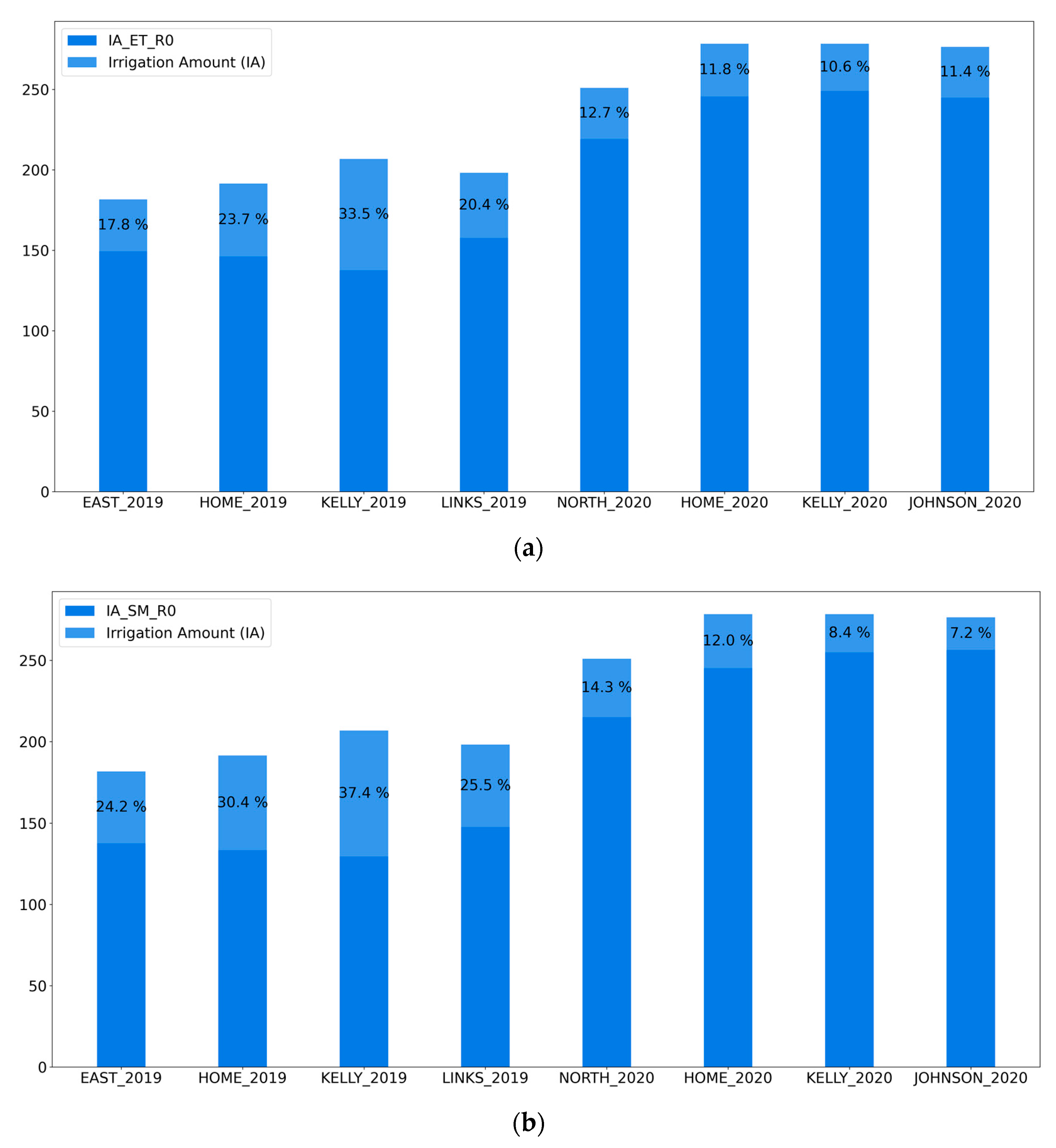
| Irrigation Amount | 149.3 | 146.1 | 137.6 | 157.6 | 219.1 | 245.6 | 249.0 | 244.8 | |
| Water Saved (%) | 17.8 | 23.7 | 33.5 | 20.4 | 12.7 | 11.8 | 10.6 | 11.4 | |
| SM | Yield | 13.8 | 14.1 | 13.3 | 12.8 | 13.3 | 13.7 | 13.9 | 13.8 |
| Irrigation Amount | 137.6 | 133.3 | 129.5 | 147.6 | 215.0 | 245.1 | 254.9 | 256.4 | |
| Water Saved (%) | 24.2 | 30.4 | 37.4 | 25.5 | 14.3 | 12.0 | 8.4 | 7.2 | |
| Year | 2019 | 2020 | |||||||
|---|---|---|---|---|---|---|---|---|---|
| Site | East | Home | Kelly | Links | North | Home | Kelly | Johnson | |
| Actual | Yield | 13.5 | 13.9 | 13.4 | 12.8 | 13.3 | 13.6 | 13.7 | 13.9 |
| Irrigation Amount | 181.6 | 191.5 | 206.8 | 198.1 | 251.0 | 278.4 | 278.4 | 276.4 | |
| ET-WB | Yield | 13.6 | 14.1 | 13.3 | 12.8 | 13.3 | 13.7 | 13.6 | 13.7 |
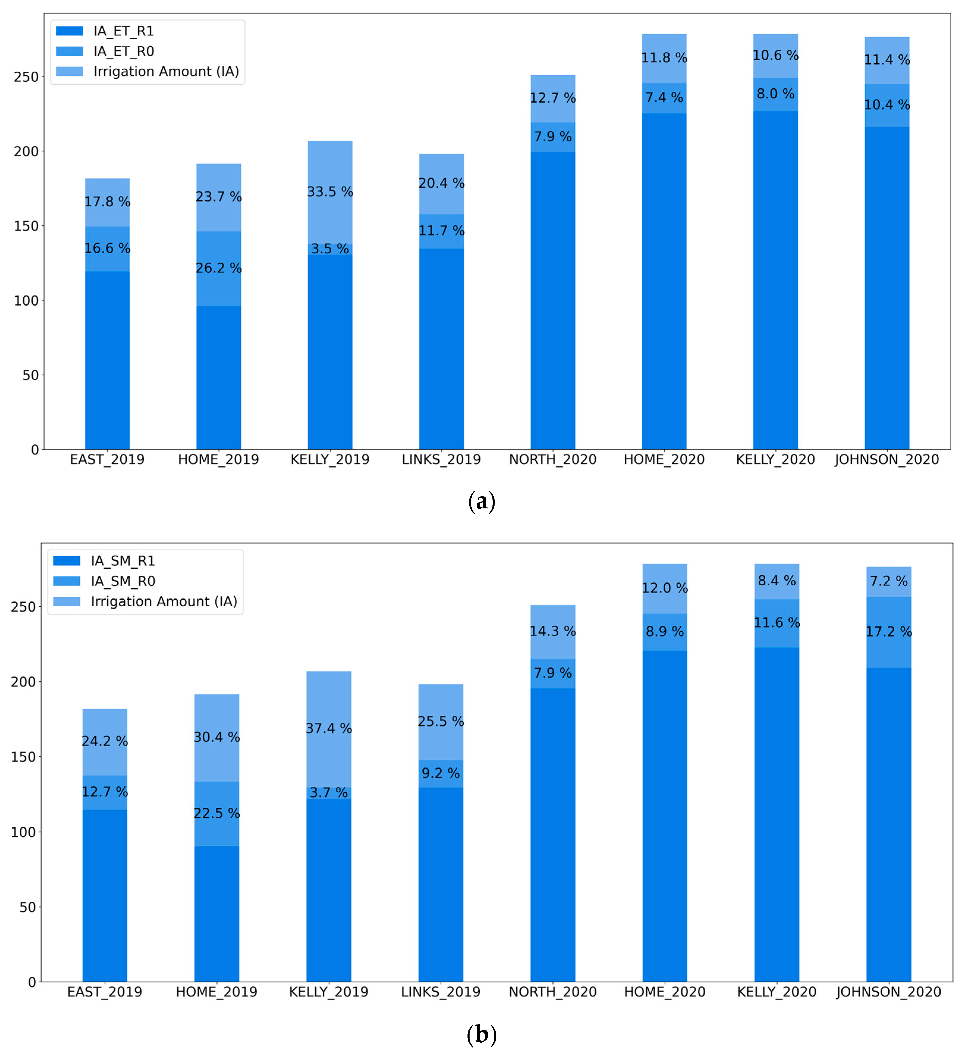
| Irrigation Amount | 119.2 | 95.9 | 130.3 | 134.4 | 199.2 | 225.0 | 226.7 | 216.1 | |
| Water Saved (%) | 34.4 | 50.0 | 37.0 | 32.2 | 20.6 | 19.2 | 18.6 | 21.8 | |
| SM | Yield | 13.6 | 14.0 | 13.3 | 12.8 | 13.3 | 13.6 | 13.6 | 13.7 |
| Irrigation Amount | 114.6 | 90.3 | 121.8 | 129.4 | 195.2 | 220.4 | 222.5 | 208.9 | |
| Water Saved (%) | 36.9 | 52.8 | 41.1 | 34.7 | 22.2 | 20.8 | 20.1 | 24.4 | |
Disclaimer/Publisher’s Note: The statements, opinions and data contained in all publications are solely those of the individual author(s) and contributor(s) and not of MDPI and/or the editor(s). MDPI and/or the editor(s) disclaim responsibility for any injury to people or property resulting from any ideas, methods, instructions or products referred to in the content. |
© 2023 by the authors. Licensee MDPI, Basel, Switzerland. This article is an open access article distributed under the terms and conditions of the Creative Commons Attribution (CC BY) license (https://creativecommons.org/licenses/by/4.0/).
Share and Cite
Zhao, H.; Di, L.; Guo, L.; Zhang, C.; Lin, L. An Automated Data-Driven Irrigation Scheduling Approach Using Model Simulated Soil Moisture and Evapotranspiration. Sustainability 2023, 15, 12908. https://doi.org/10.3390/su151712908
Zhao H, Di L, Guo L, Zhang C, Lin L. An Automated Data-Driven Irrigation Scheduling Approach Using Model Simulated Soil Moisture and Evapotranspiration. Sustainability. 2023; 15(17):12908. https://doi.org/10.3390/su151712908
Chicago/Turabian StyleZhao, Haoteng, Liping Di, Liying Guo, Chen Zhang, and Li Lin. 2023. "An Automated Data-Driven Irrigation Scheduling Approach Using Model Simulated Soil Moisture and Evapotranspiration" Sustainability 15, no. 17: 12908. https://doi.org/10.3390/su151712908