Discrete Choice Experiment Consideration: A Framework for Mining Community Consultation with Case Studies

Abstract

Local community acceptance, a key indicator of the socio-political risk of a project, is addressed through good stakeholder (community) engagement. Discrete choice modeling (DCM) enhances stakeholder analysis and has been widely applied to encourage community engagement in energy projects. However, very little detail is provided on how researchers design discrete choice experiments (DCEs). DCE design is the key step for effective and efficient data collection. Without this, the discrete choice model may not be meaningful and may be misleading in the local community engagement effort. This paper presents a framework for mining community engagement DCE design in an attempt to determine (1) how to identify the optimum number of factors and (2) how to design and validate the DCE design. Case studies for designing discrete choice experiments for community acceptance of mining projects are applied to accommodate these two objectives. The results indicate that the four-factor design, which seeks to reduce cognitive burden and costs, is the optimal choice. A survey was used to examine the difficulty of the survey questions and the clarity of the instructions for the designs. It has, therefore, been proven that the DCM design is of reasonable cognitive burden. The results of this study will contribute to a better design of choice experiments (surveys) for discrete choice modeling, leading to better policies for sustainable energy resource development.

1. Introduction

While the impact of energy on society is overwhelming, the juxtaposition of adverse environmental and social impacts cannot be ignored in a holistic discussion. Over the past few decades, concerns over sustainable development have increased around the world [1,2,3,4]. As global expectations have changed the role of business, the energy industry cannot continue to undertake projects as it has in the past.

As Rotheroe et al. put it, “sustainable development can only be given real meaning by interrogating the ideas through a multi-stakeholder approach” [3]. It is increasingly evident that community engagement is important to the successful implementation of energy resource projects for both private, for-profit organizations and public institutions (who regulate resource projects and create policies to enable the sustainable development of energy resources). Organizations like the International Council on Mining & Metals (ICMM) and the International Finance Corporation (IFC) have discussed stakeholder engagement to varying degrees. Stakeholder engagement includes three main parts: stakeholder identification, stakeholder analysis, and iterative consultation [5]. The most widely used method for stakeholder analysis in mining is recommended by the ICMM [6]. This technique involves the analyst(s) assessing each stakeholder’s perspective on the project (negative, neutral, positive), their level of influence (low, medium, high), and the extent to which the project will affect them (low, medium, high). Stakeholders are then divided into three groups: those who are extremely influential opponents of the project, those who are neutral on the project, and those who are highly influential supporters of the initiative. During the iterative consultation process, the outcome of stakeholder analysis is crucial and offers the key to analyzing stakeholder perspectives on an energy resource project. Thus, stakeholder analysis affects the entire stakeholder engagement process.

Current qualitative community analysis methods alone may not provide sufficient insight into the community’s concerns, needs, and level of acceptance to achieve the goals of the community analysis process. Additional (qualitative or quantitative) methods that provide unique insight can help provide information that is not currently available. This will ensure that the energy sector targets the right people in the community and focuses on the right issues in its community engagement. There is a need for some quantitative methods, including computer modeling, to augment the current qualitative methods.

Discrete choice theory is a quantitative method for stakeholder analysis that has been successfully applied to evaluate community acceptance of various energy projects [7]. There are four types of typical discrete choice models that can be proposed in empirical investigations, namely the multinomial logit (MNL) model, the nested logit (NL) model, the heteroscedastic extreme value (HEV) model, and the mixed logit model. For instance, discrete choice models (DCMs) have been applied to assess the local acceptability of wind-farm investment [8], efficient management of biodegradable waste [9], Lithuanian households’ preferences for different microgeneration technologies [10], and a coal mining project in Australia [11,12].

DCE design is important because DCE results cannot be valid if the design produces flawed instruments that do not elicit respondents’ true preferences. Details of how to conduct a DCE and the associated theoretical issues have been well covered in previous literature. For example, Grasshoff et al. introduce a novel model based on probit part-worth utilities which can account for similarities in the alternatives by supposing a dependence structure [13]. Also, Traets et al. present a new R package, called idefix, which enables users to generate Bayesian adaptive designs which can be used to gather data for the mixed logit model [14]. Thai et al. show a promising future use of partial choice set design (PCSD) by providing evidence that PCSD can reduce cognitive burden while satisfying convergent validity compared to full choice set design (FCSD) [15]. Mamine et al. present a meta-analysis that explores the impact of methodological choices related to the timing of the DCE (design stage, implementation stage, and analysis stage) on farmers’ contract preferences regarding the adoption of agrienvironmental practices [16].

One of the main considerations in designing DCEs is determining how to ensure the design is clearly understood by the respondents. The discrete choice modeling result can be invalid if the participants are confused by the design. This consideration leads to two questions that have not been well addressed in the literature. First, how does one identify the optimum number of factors? Designing DCEs with too many attributes can result in choice sets that place too high of a cognitive burden on respondents. Second, how does one design and validate the DCE design? Fewer researchers have reported on experimental design and validation before sending out discrete choice experiments (DCEs). The designs of some DCEs are limited, and the “black box” nature of the design process hides these limitations. Addressing how these two questions can impact the validity of a DCE is important for understanding their value for stakeholder analyses. This research could contribute to a more reasonable DCE design and improve the understanding of the sustainability of mine operations from the mining community’s perspective.

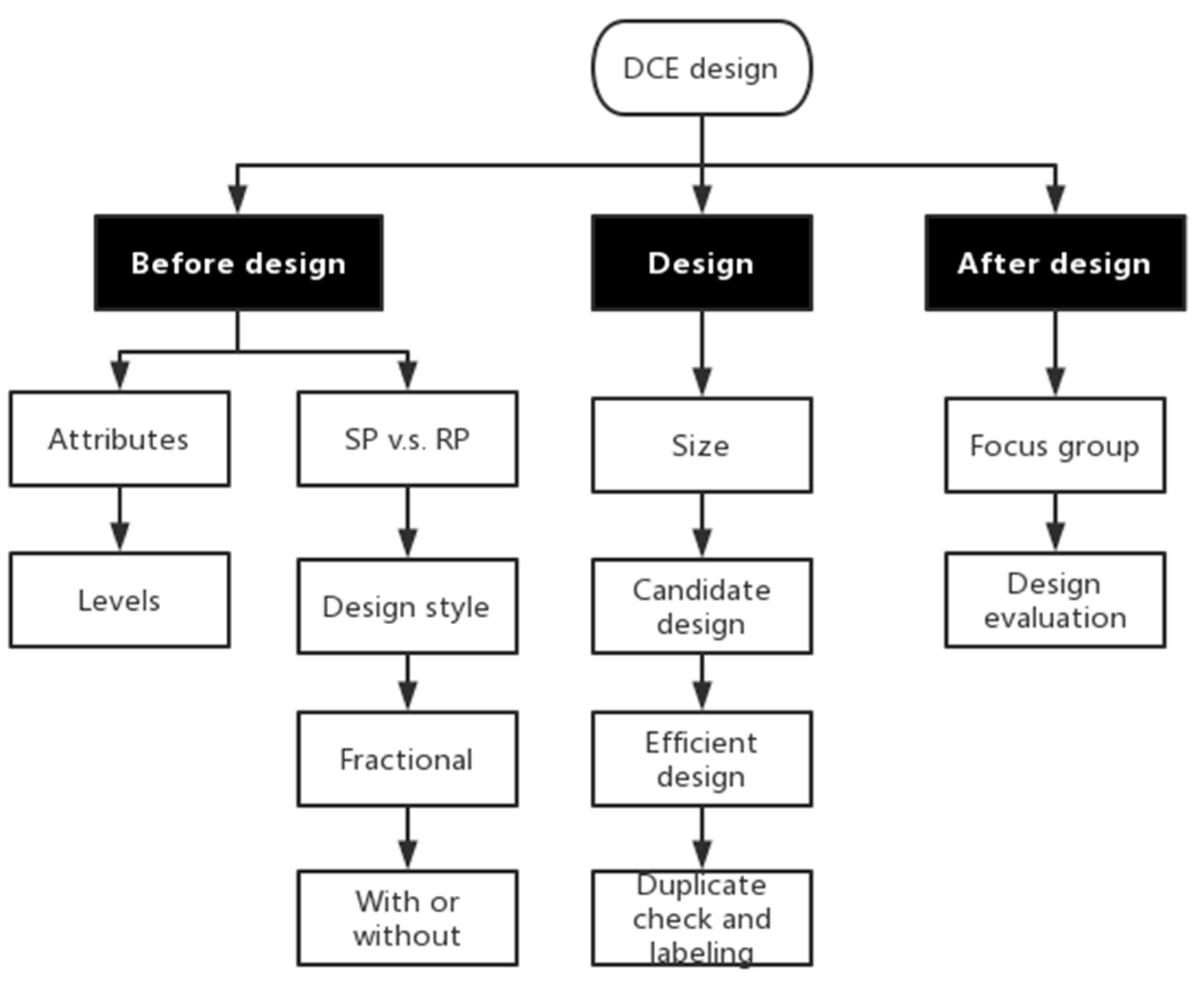
2. Materials and Methods

The framework for DCE design developed to encourage mining community engagement is shown in Figure 1 and consists of three main parts. Before the DCE design is implemented, a validated list of demographic factors with proper levels of key mining attributes needs to be identified. In addition, the DCE needs to be designed based on the factor list, followed by experimental size determination, candidate design, efficient design, duplication checking, and labeling. Finally, the results of candidate DCMs need to be validated by a focus group to evaluate the effort and difficulty rating.

2.1. Attributes and Levels

The attributes and levels per attribute are a key part of designing a choice experiment [17,18]. Firstly, the selected attributes and levels for each attribute should be essential and relevant to the choice and potential participants. Secondly, these need to be realistic and framed appropriately. Take two attributes, “job opportunities” and “income increase”, as examples. The potential “job opportunities” and “income increase” due to the presence of a mine depend on the practicality of the mine and the community where it is located. These factors should be carefully considered. In this research, all levels were determined with regard to a mine close to Salt Lake City, since the final survey was conducted there. Thirdly, the attributes and levels should be understandable to most respondents while providing useful information. For instance, an explanation may be added to the property “mine buffer” to clarify that it represents “the distance between the respondent’s residence and the mine”. Infrastructure enhancement may be exemplified by features such as transportation, education, human services, and internet connectivity.

In this study, a three-step flowchart is shown in Figure 2, and the attributes and levels for each attribute are shown in Appendix A. A detailed discussion of how the authors arrived at these attributes is contained in previous research by Que et al. [19].

2.2. Experimental Design Considerations

2.2.1. Stated Preference vs. Revealed Preference

Revealed preference (RP) and stated preference (SP) are the primary discrete choice experiment methods. RP is a conventional method, which refers to situations where the choice is made in a real market scenario. By contrast, SP refers to situations where a choice is made by considering hypothetical situations. The choice options in SP are similar to those in RP, except that the choices in RP are limited to reality. This feature results in a major advantage for SP.

The most popular method for DEC design is to utilize both RP and SP choice data [22]. In this research, the status quo option shows the average value of each attribute/characteristic in the real world. The other two alternatives in the choice set use the same attributes but different combinations of attribute levels to generate hypothetical situations. The design of this study is, consequently, a mixed design, as recommended by Louviere, Hensher, and Swait [23]. Thus, we can show participants various real and hypothetical mining scenarios [24].

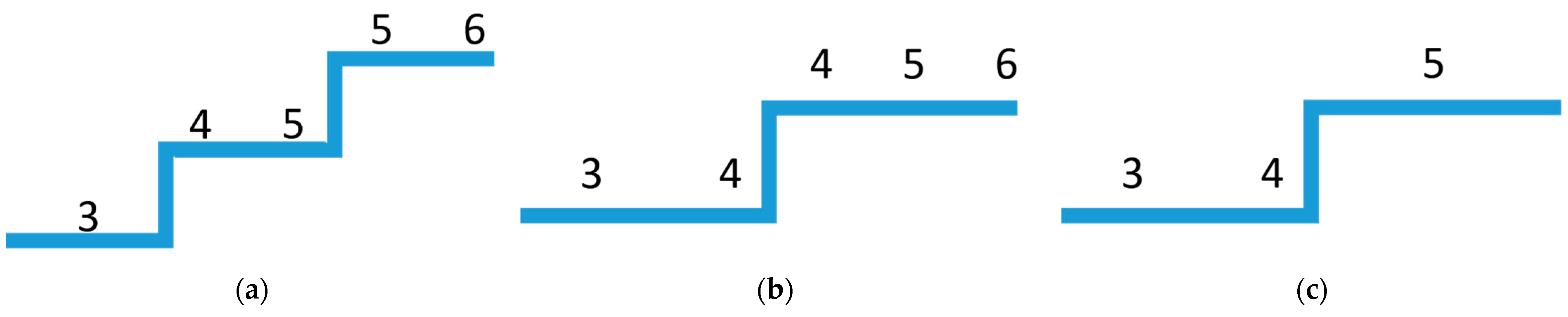
2.2.2. Block Scheme Design

Block scheme design is a method that can be used when there are numerous attributes due to respondent burden and/or sample size considerations. In a block scheme design, these attributes are partitioned into several independent discrete choice experiments. It is an essential new strategy to explore because reducing the number of qualities utilized is not always practical or desired.

There are two reasons why the number of traits is kept to a minimum [25]. Firstly, due to the significant variety of attributes, individuals may use other decision-making lexicographic or heuristic rules instead of making trade-offs. This result contradicts a crucial assumption of economic choice theory, which states that the data cannot be interpreted as a utility [26]. For responders who are more likely to use compensating choice rules, a reduced number of qualities minimizes task complexity. The choice sets are constructed with reasonable factors, which reduces the cognitive burden placed on respondents. A cognitively demanding set may cause respondents to randomly select a choice rather than make a rational decision.

The second rationale for having fewer attributes is that it is more practical; the fewer the permutations of levels and attributes, the fewer the choice sets that must be offered. This eliminates the need to block choice sets across multiple versions of the questionnaire, lowering the sample size necessary to complete a given number of choice sets and, as a result, lowering the cognitive load of the choice tasks. The full combination of 16 factors, each with three levels, is 3¹⁶ = 43,046,721. If the factors are split into four blocks of four attributes each, the full combination will be 3⁴ × 4 = 324. This means that not only will researchers save huge amounts on survey costs, but each participant will also deal with much fewer choice sets.

Blocking is commonly used to decrease the quantity of choice sets that every respondent has to answer, thereby reducing the number of attributes. Witt, Scott, and Osborne [27] used a block scheme design in a choice experiment with eleven attributes, of which ten have four levels, and one has three levels. Instead of presenting each respondent with all eleven attributes, the attributes were “blocked” into three experimental designs.

2.2.3. Fractional Factorial Design

Fractional factorial design refers to survey designs that use only a fraction of the total number of treatment combinations. If each block has four factors with three levels in the DCE design, the full set of combinations will be 81 = 34. This means we will have more than 40 choice sets (each choice set includes two hypothetical alternatives plus the status quo option) for each block. This number of questions (each choice set will be presented as a question) is too high. Thus, a fractional factorial design is used in this case study [23,24].

2.2.4. Interaction vs. No Interaction

A discrete choice experiment can examine both primary factors and interactions. In this study, the design only includes the main factors because interactions rarely account for much of the choice. The main effects typically account for 70% to 90% of the explained variance, while two-way interactions typically account for 5% to 15%, and higher-order interactions account for the remaining explained variance [23].

2.3. Challenges and Methods in the Developed Framework

The developed framework needs to accommodate two challenges in designing discrete choice experiments for community acceptance of mining projects: (1) the need to identify the optimum number of factors to ensure the resulting DCE design is valid and (2) the need to design and validate the DCE in a manner that is appropriate for the participants.

2.3.1. How to Identify the Optimum Number of Factors

Before using a block scheme design to account for a large number of factors in discrete choice experiments for mining community acceptance evaluation, there is a need to investigate the optimal number of factors for one choice set. Without this, the blocking scheme may still be too burdensome (as there are still too many attributes in each choice set) or inefficient (as there are too few factors in each choice set) for the respondent, leading to higher-than-necessary costs. In order to accommodate this challenge, discrete choice experiments need to be designed with a different number of factors, from three to six, for this study.

Factors were selected from the 16 factors validated in Appendix A by including one factor from each of the four categories (economic, social, environmental, and governance) and balancing the positive, negative, and neutral effects. The factors included in each design and their levels are shown in Table S1. Respondents were asked to rate the required effort and difficulty of each choice set, and these ratings were tracked for each design to find the optimal number of factors.

2.3.2. How to Structure and Validate a DCE Design

As discussed in Section 2.2, the discrete choice experiment will be designed as a mixed-style, fractional factorial blocking scheme without interaction. This design has five main steps: determine the size of the experiment, construct the candidate design, design an efficient experiment, check for duplicates, and label. The functions and respective SAS macros are shown in

Table 1. Steps for generating experiments.

Step	SAS Macro	Function
1. Experimental size determination	%MktRuns [28]	Suggests sizes for balanced fractional factorial experiment designs
2. Candidate design construction	%MktEx [29]	Creates efficient factorial designs with the selected size
3. Efficient experiment design	%ChoicEff [30]	Finds optimal experimental designs for evaluating choice designs and choice experiments
4. Duplicate check	%MktDups [31]	Alternatives within the generic choice set and detects duplicate choice sets
5. Labeling	%MktLab [32]	Labels factors and their levels for each block

.

In the validation step, a focus group was used to examine the difficulty of the survey questions and the clarity of the instructions. A choice-set sample is shown in

Table 2. Example of choice sets.

	Income Increase	Population Increase	Mine Life	Air Pollution	I Would Choose
Option 1	+$300 per month	Continued population growth (average rate 4%)	20 years	A slight increase in pollution
Option 2	+$100 per month	Continued population growth (average rate 4%)	30 years	No increase in pollution
Option 3	+$500 per month	A reduced rate of population growth (only 2%)	20 years	A moderate increase in pollution
Option 4	Too complex to decide

. Participants were asked to choose one of three mining options if a new mine were to open in their neighborhood. Each choice set has four alternatives: Option 4 is “Too complex to decide”. Following each question, participants were asked to rank their level of perceived confusion and difficulty by selecting a number from 1 (“not difficult at all”/“not confusing at all”) to 5 (“very difficult”/“very confusing”). After completing the questions in each DCE design, participants were asked to assess the perceived difficulty of the choice experiments with three, four, five, and six factors (i.e., four difficulty ratings). The same seven levels (from very easy to very difficult) were used in the difficulty rating. The system kept track of how long each participant took to complete each design.

2.4. Statistical Data Analysis and Case Study Survey

2.4.1. Kruskal–Wallis Test

The Kruskal–Wallis test is a non-parametric statistical test used to compare the medians of three or more independent groups. It assumes that these groups are sampled from populations with the same median (null hypothesis) and suggests that at least one group has a different median (alternative hypothesis). When the p-value obtained from the Kruskal–Wallis test is below a predetermined significance level (such as 0.05), the null hypothesis is rejected, indicating that there are differences in medians between at least one pair of groups. In discrete choice models, the Kruskal–Wallis test can be applied to compare the impact of different levels of explanatory variables on the choice behavior of a dependent variable with ordinal characteristics and to compare differences in medians among different groups.

2.4.2. Dunn’s Multiple Comparison Test

Dunn’s multiple comparison test is a non-parametric method used to compare pairwise differences among multiple groups. In discrete choice experiments, when the data are continuous or ordinal, the Kruskal–Wallis test rejects the null hypothesis (indicating median differences among at least one pair of groups), and the data are classified as tied ranks, a Dunn’s multiple comparison test can be applied. The test allows for comparisons between specific groups or levels to determine significant differences in choices based on different attributes or levels of the independent variable.

2.4.3. Case Study Survey

An online survey was conducted to validate the design of the DCE. The survey began with a series of basic background questions regarding demographics, the respondents’ socioeconomic status, and their past experience with mining. The demographic questions also included age, gender, income, and education level. In this survey, participants were asked to select one of three design choices if a new mine were to be opened in their community. Following the questions regarding each design, participants were asked to rank the level of effort and difficulty of each design by selecting a number from 1 to 7 (“not difficult at all” to “very difficult”).

Twenty-five people participated in the focus group survey, and twenty-two of them completed it (i.e., answered all questions). Although the sample size may seem small, this is consistent with focus groups in general, which tend to have small sample sizes since they are only preliminary [33]. The data were regarded as invalid if the participant completed the survey in less than one-third of the average survey time (seven minutes for this survey). No participant finished in less than the minimum time. Two participants “failed” basic quality control questions, which asked participants to answer simple questions about the tasks they had just completed, and data from these two participants were deleted. Thus, data from 20 participants were used for the subsequent data analysis.

3. Results

3.1. Case Study for Challenge One

In this study, effort and difficulty level ratings were acquired for questions from all four designs. The degree of effort and difficulty ratings for these four designs were compared using statistical analysis to determine if there was a significant difference in ratings. Data from the effort and difficulty level assessments for the four designs were considered separate groups. The Kruskal–Wallis test was chosen for this case study since data on the level of difficulty and effort were represented as ordinal in this situation [34]. Nemenyi and Dunn’s multiple comparison tests were based on significant Kruskal–Wallis test results. In this case, Dunn’s multiple comparison test was used since the data are classified as tied ranks.

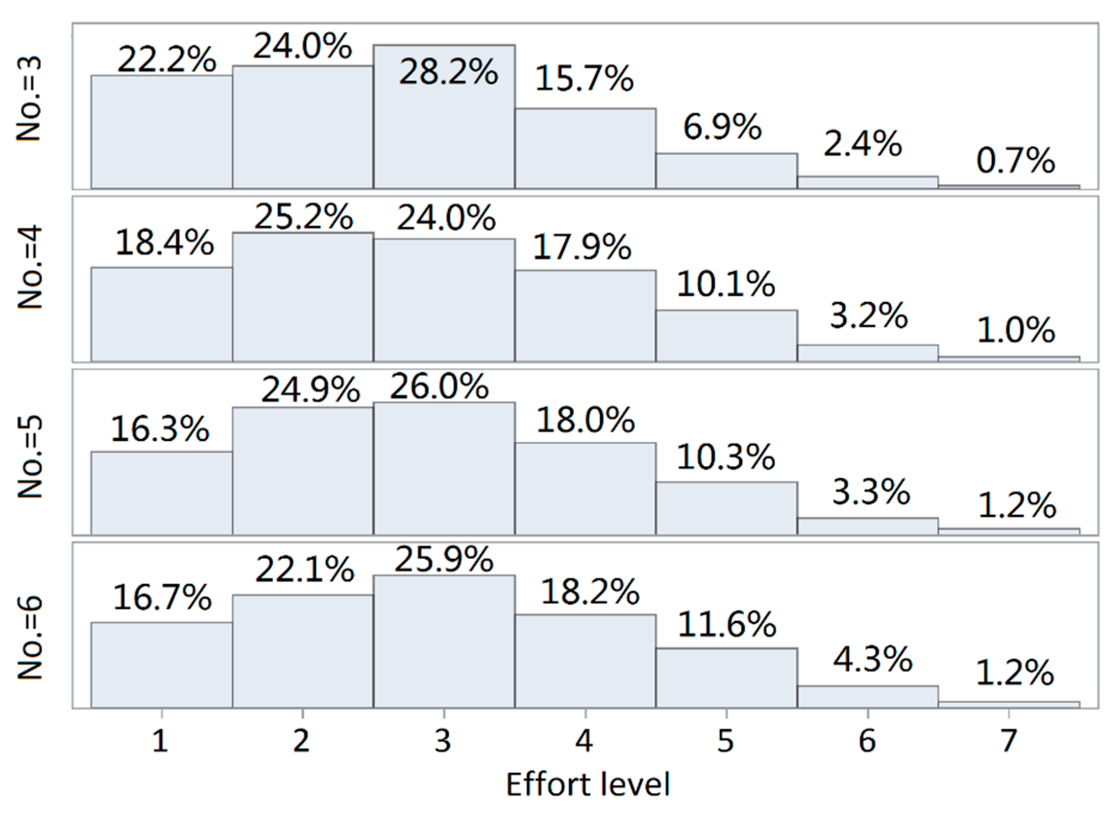
3.1.1. Effort Level Analysis

The effort level rating distributions are shown as histograms in Figure 3. All the distributions are relatively asymmetric and skewed to the left. Most of the participants selected level 2 (Easy) or level 3 (Somewhat easy) effort ratings for all four designs, with the number of factors ranging from three to six. As the number of factors increased from three to six, the percentage of respondents selecting level 4 (Neutral) increased from 15.7% to 18.2%. Similarly, the percentage of respondents selecting levels 5, 6, and 7 increased from 6.9% to 11.6%, 2.4% to 4.3%, and 0.7% to 1.2%.

The Kruskal–Wallis test was performed using the SAS PROC NPAR1WAY WILCOXON procedure [35] to evaluate whether there is a significant difference between the four designs. The p values were estimated at <0.0001, which means the test rejected the null hypothesis. At the significance level of 0.05, it may be determined that there is at least one significant difference between the effort level ratings of these four designs.

Dunn’s multiple comparisons were used to find the detailed differences between each pair of designs [34,36]. As shown in

Table 3. Results of the Dunn’s multiple comparisons test for effort level ratings.

Comparison Group = Number of Factors
Compare	Diff	SE	QAB	Q(0.05)	Conclude
6 vs. 3	459.81	68.08	6.75	2.638	Reject
6 vs. 4	197.71	68.08	2.90	2.638	Reject
6 vs. 5	104.80	68.08	1.54	2.638	Do not reject
5 vs. 3	355.01	68.08	5.21	2.638	Reject
5 vs. 4	92.91	68.08	1.36	2.638	Do not reject
4 vs. 3	262.10	68.08	3.85	2.638	Reject

, the Q critical value is 2.638 at a significance level α = 0.05. The effort level ratings of the three-factor designs are significantly different from those of the other three designs. The calculated QAB statistics (3.85, 5.21, and 6.75) exceed the Q critical value. Moreover, the effort level ratings of the four-factor design are significantly different from those of the six-factor design (QAB = 2.90). However, the effort level ratings of the four-factor design are not significantly different from those of the five-factor design (QAB = 1.36), and the effort level ratings of the five-factor design are not significantly different from those of the six-factor design (QAB = 1.54).

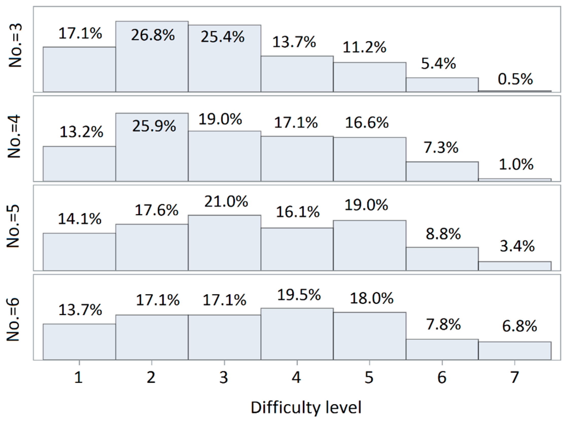
3.1.2. Difficulty Level Analysis

The difficulty level rating distributions are shown in Figure 4. The mode of distribution for the three- and four-factor designs is level 2 at 26.8% and 25.9%; for the five-factor designs, it is level 4 at 21.0%; and for the six-factor designs, it is level 5 at 19.5%. For the three-factor design, the distribution is relatively asymmetric and skewed to the left. However, as the number of factors increases, the distribution becomes less and less skewed to the left. The distribution of the six-factor design is nearly symmetric.

The same Dunn’s multiple comparisons and Kruskal–Wallis test were used to analyze whether or not the number of factors included in one choice set had a significant effect on the difficulty level ratings. When α = 0.05 (p = 0.0003), the null hypothesis of the Kruskal–Wallis test was rejected. The results show that there are obvious differences among the four designs. The result of Dunn’s multiple comparisons is shown in

Table 4. Results of the Dunn’s multiple comparisons test for difficulty level ratings.

Comparison Group = Number of Factors
Compare	Diff	SE	QAB	Q(0.05)	Conclude
6 vs. 3	92.87	23.02	4.03	2.638	Reject
6 vs. 4	48.40	23.02	2.10	2.638	Do not reject
6 vs. 5	Do not reject (within non-sig. comparison)
5 vs. 3	77.25	23.02	3.36	2.638	Reject
5 vs. 4	Do not reject (within non-sig. comparison)
4 vs. 3	44.47	23.02	1.93	2.638	Do not reject

. The Q critical value is 2.638, while the significant level is 0.05.

While the difficulty level ratings of the three-factor design are not significantly different from those of the four-factor design (QAB = 1.93), they are significantly different from those of the designs with five and six factors. The calculated QAB statistics (3.36 and 4.03, respectively) exceed the Q critical value. The difficulty level ratings of the four-factor design are not significantly different from those of the six-factor design (QAB = 2.10). In addition, the pair-wise comparison of difficulty level ratings for five-factor vs. four-factor and six-factor vs. five-factor designs shows no significant differences.

3.1.3. Analysis Based on Duration of the Survey

We recorded the time it took each participant to complete the survey portion of the design, and Figure 5 shows a comparative box plot. In all four designs, the average duration was higher than the median. The median and mean time durations of the design with three factors are 30 and 22 s, respectively. For the design with four factors, both the mean and median decrease slightly to 29 and 21 s, respectively. Further, the median and mean increase to the highest values for the design with five factors at 33 and 27 s, respectively. For the design with six factors, both the median and mean fall rapidly to their lowest values at 25 and 20 s, respectively.

Dunn’s multiple comparisons and the Kruskal–Wallis test were used to analyze whether or not the number of factors included in one choice set had a significant effect on the survey duration. The null hypothesis of the Kruskal–Wallis test was rejected at α = 0.05 (p < 0.0001). The results show obvious differences in the survey duration among the four designs, as can be seen in

Table 5. Results of the Dunn’s multiple comparisons test for survey duration.

Comparison Group = Number of Factors
Compare	Diff	SE	QAB	Q(0.05)	Conclude
5 vs. 3	87.27	23.22	3.76	2.638	Reject
5 vs. 4	111.33	23.22	4.79	2.638	Reject
4 vs. 3	24.06	23.22	1.04	2.638	Do not reject

.

As shown in Table 5, there are no obvious differences among the survey durations for designs with three and four factors (QAB = 1.04). This finding was confirmed by the fact that there was no obvious difference in difficulty rating between the two designs. In Figure 5 it appears that the duration of the design with four factors is slightly less than that of the design with three factors. The respondents may be learning when they conduct the survey. Caussade et al. observed a learning effect in choice situations [18]. Although the four-factor design has one additional factor, the questions, choice of style, and framework are the same.

In addition, the survey duration of the design with five factors is significantly different from those with three and four factors. The calculated QAB statistics (3.76 and 4.79, respectively) exceed the Q critical value (2.638). The design with six factors is unique in the survey duration analysis. In Figure 5, the survey duration drops sharply to the lowest timeframe at 25 and 20 s, respectively. It is likely that the design with six factors is too complicated, and participants are randomly selecting the choices. Thus, the duration data from this design are treated as invalid and were not used in Dunn’s multiple comparison test or the Kruskal–Wallis test.

3.1.4. Comparison

Firstly, participants indicated that designs with fewer factors required less mental effort, and the choices were easier to make. As the number of factors increased, both the perceived level of required mental effort and the perceived difficulty increased. The result of Kendall’s correlation analysis appears to support the fact that the number of factors and the frequency of “too complex to choose” are positively correlated, with a correlation coefficient of 0.0503. Although the magnitude of the correlation coefficient may seem negligible, the existence of such a correlation appears to be supported by the effort and difficulty rating data. These findings support our hypothesis that a higher number of factors will lead to greater amounts of cognitive load (e.g., higher effort and difficulty ratings).

In addition, the Kruskal–Wallis test results showed significant differences between the participants’ effort ratings, difficulty ratings, and survey duration for these four designs at a significance level of 0.05. The results of Dunn’s multiple comparison tests, which were used for the pairwise comparison of the designs, are summarized in Figure 6a–c.

As shown in Figure 6a,b, there is no significant difference between designs with five and six factors for either effort or difficulty level ratings. As shown in Table 4 and Figure 4, the design with six factors is not as easy compared to the other three designs. Almost 10% (specifically, 8.69%) of the time, respondents indicated that choice sets with six factors are too complex to make a decision. The difficulty level rating mode for this design is level 4 (neutral), and 52.1% of the time, respondents indicated that choice sets with six factors are at a “neutral” (neither difficult nor easy) level of difficulty or are difficult. These results indicate that the designs with five and six factors are not good options for the block scheme experimental design.

The design with three factors is the easiest among these four designs. Only 4.62% of the responses indicated that the questions with three factors were “too complex” to make a decision. Moreover, 74.4% and 69.3% of the time, respondents indicated that the effort and difficulty level of these choice sets, respectively, were equal to or less than level 3 (somewhat easy). While the design with four factors requires relatively more effort and is ranked as more difficult than the design with three factors, it is still easy enough for the block scheme experimental design. Further, 67.6% and 58.1% of the time, respondents indicated that the effort and difficulty level ratings, respectively, were equal to or less than level 3 (somewhat easy). In addition, there is no significant difference between the designs with three and four factors regarding both difficulty level and survey duration, as shown in Figure 6b,c. Based on these results, both the three- and four-factor designs are good options for the block scheme experimental design. The lower the number of factors included in one choice set, the more blocks are needed in the block scheme experimental design, which will increase the cost of the overall survey. Thus, the design with four factors is the optimal choice to reduce the cognitive burden and reduce costs.

3.2. Case Study for Challenge Two

3.2.1. Design Generating Experiments

In this case study, the 16 mining characteristics were separated into four blocks. Each block includes one factor from each of the four categories, and the factors are chosen to balance the positive and negative effects (Table S2). There are three positive impacts included in the 16 characteristics, with the exception of Block 4. However, participants will understand that the main objective is to make trade-offs, assuming all other factors were at status quo levels in the previous blocks.

• Experimental Size Determination

The size of the experiment needs to be determined to achieve perfect orthogonality and balance or, at least, to minimize violations of balance and orthogonality in the following experimental design. The design is orthogonal when all parameter estimates are uncorrelated. When all levels of each factor occur equally often, the design is balanced. The relative D efficiency ranges from 0% to 100% (Equation (1)) and is an indicator of the effectiveness (orthogonality and balance) of discrete choice experiments [37]. The design size is selected to achieve the maximum possible relative D-efficiency.

$$\mathrm{Relative}\mathrm{D}\text{-}\mathrm{efficiency}=\frac{1}{{\left|\mathsf{\Sigma }\right|}^{1/\mathrm{K}}\times \mathrm{n}\mathrm{u}\mathrm{m}\mathrm{v}\mathrm{e}\mathrm{r}\mathrm{o}\mathrm{f}\mathrm{c}\mathrm{h}\mathrm{o}\mathrm{i}\mathrm{c}\mathrm{e}\mathrm{s}\mathrm{e}\mathrm{t}\mathrm{s}}\times 100\%$$

(1)

where ∑—the covariance matrix of choice set design.

K—the number of parameters.

The SAS% MktRuns macro was used to determine the design size with four factors, each with three levels [28]. The possible sizes and corresponding relative D-efficiencies are shown in

Table A1. Experimental size suggestion output.

Saturated = 9
Full Factorial = 81
Observation	Reasonable design size
1	9 *,S
2	18 *
3	12
4	15
5	10
6	11
7	13
8	14
9	16
10	17

*—100% efficient design.; ^S—Saturated Design—the smallest design that can be made.

. The saturated design size (the smallest design that can be made) is 9, and the full design size is 81. Designs with 100% relative D-efficiency can be achieved with sizes 9 and 18. Both satisfy the desire for a reasonable sample size and maximize the relative D-efficiency. In this study, each question (choice set) includes the status quo alternative and two hypothetical alternatives. Thus, the authors chose a design size of 18 since 18 hypothetical alternatives can be divided into nine choice sets of two alternatives each.

• Candidate design construction

In this step, the researcher must construct a candidate design with the design size selected in the experimental size determination. Meyer and Nachtsheim’s [38] coordinate-exchange algorithm (CoordX) provides a way to search the candidate designs by initializing the design with an orthogonal and random design [37]. The CoordX algorithm will stop if it finds a perfect, orthogonal, 100% efficient, and balanced design [29]. The solution (candidate design) is shown in

Table A2. CoordX algorithm output (100% efficient).

Observation	x1	x2	x3	x4
1	1	1	1	1
2	1	1	2	2
3	1	2	1	3
4	1	2	3	1
5	1	3	2	3
6	1	3	3	2
7	2	1	1	3
8	2	1	3	1
9	2	2	2	2
10	2	2	3	3
11	2	3	1	2
12	2	3	2	1
13	3	1	2	3
14	3	1	3	2
15	3	2	1	2
16	3	2	2	1
17	3	3	1	1
18	3	3	3	3

. The CoordX algorithm, as implemented in the SAS% ChoicEx macro, was used to find a candidate design with 100% D-efficiency.

• Efficient experiment design

In this step, the hypothetical alternatives need to be divided into several choice sets of two alternatives each (each choice set consists of two hypothetical alternatives plus a status quo option). A modified Fedorov (MFed) candidate-set-search algorithm was used in this step [37] to construct a random initial design from the candidate design. This was then evaluated by exchanging alternatives/sets until the D-efficiency stabilized at a local maximum. In order to determine the best design for all possible initial designs, this process was repeated for different initial designs.

The MFed algorithm was implemented in the SAS% ChoicEff macro, which was used to find the most efficient random scheme to pair the 18 alternatives into nine choice sets [30]. The process was repeated with 145 initial designs. The candidate-set-search output is shown in

Table A3. Sample candidate-set-search results.

Design	Iteration	D-Efficiency	D-Error	Relative D-Efficiency
1	0	0	.	.
	1	5.970687	0.167485	66%
	2	6.142330	0.162805	68%
	3	6.500560	0.153833	72%
	4	6.500560	0.153833	72%
2	0	1.837117	0.544331	20%
	1	5.759409	0.173629	64%
	2	5.845501	0.171072	65%
	3	6.167149	0.162149	69%
	4	6.167149	0.162149	69%

, which shows two runs, with both converging in four iterations. The first run in Table A3 returns the maximum D-efficiency and corresponds to the pairing shown in

Table A4. The efficient experimental design result.

Observation (Table A2)	Set
4	1
13	1
8	2
15	2
9	3
18	3
16	4
11	4
12	5
3	5
5	6
14	6
17	7
2	7
1	8
10	8
6	9
7	9

.

The relative D-efficiency is 72%. This step changes the relative D-efficiency (from 100%) since it depends on the number of choice sets (Equation (1)). The authors deemed this adequate for the purposes of this study. If the relative D-efficiency is too low, the designer can change the size of candidate alternatives or the number of choice sets to improve the design. The number of levels for each attribute and the number of attributes can also affect the relative D-efficiency. However, these are difficult or unrealistic to change in real life.

• Duplicate check and labeling

During this step, the design needs to be checked for duplicate choice sets and alternatives. The experimental design needs to be labeled with a full description of factors and their levels for each block. The SAS% MktDups macro was used to check for duplicates [31], while the SAS% MktLab macro was used to label the experiments with factors and levels [32]. There were no duplicate choice sets or alternatives inside the option sets in this scenario.

3.2.2. Design Validation

In this focus group study, the authors used the survey to examine the difficulty of the survey questions and the clarity of the instructions for all four blocks. The data analysis method was the same as that used in case study 1. When the significant level is 0.05, the Kruskal–Wallis test fails to reject the null hypothesis. The p-values were estimated as 0.9536, 0.8469, and 0.6373 separately. This result means that there is not enough evidence to prove that there is at least one significant difference between difficulty level, confusion level, and the duration of the survey for respondents on these four blocks at a significant level of 0.05. The result is shown in

Table 6. Level of difficulty/confusion scale for each block.

	Confusing Level	Difficulty Level
Block 1	(2, 4)	(2, 4)
Block 2	(2, 3)	(2, 3)
Block 3	(2, 3)	(2, 3)
Block 4	(2, 3)	(2, 3)

1 Not difficult/confusing at all; 2 Not very difficult/confusing; 3 Acceptable; 4 Somewhat difficult/confusing.

. Furthermore, the median level of difficulty and confusion rating for all blocks (2, 3) were above “not very difficult/confusing” but below “acceptable” and (2, 4) above “not very confusing” but below “somewhat confusing,” respectively. As a result, the DCE design accomplishes one of the key aims of all blocks’ issues, namely that the survey is not too difficult (i.e., reasonable cognitive burden).

Although there is no statistical difference between the confusion and difficulty ratings of the four blocks, the results showed that Block 1 has a slightly higher rating than the other three blocks. The time duration analysis confirmed this finding: both the mean peaked and the median are at Block 1. However, when respondents proceed through the survey, it is also likely that they are learning as they go. Caussade et al. discovered that, in certain circumstances, there is a learning impact [18]. Though the factors are different, the choice of style, the question, and the framework remain the same. Therefore, these four blocks should be randomly ordered in the actual discrete choice experiment. In this way, unnecessary variance in DCM can be avoided.

4. Discussion

In this study, the authors proposed an approach to overcome two challenges of DCE design for mining community engagement. The challenges then are (1) how one can identify the optimum number of factors and (2) how one can develop and validate the DCE design. The approach is based on incorporating all important characteristics (16 in this work) into discrete choice experiments by using block scheme designs, in which factors are split into several discrete choice experiments. A survey was used to examine the difficulty and clarity of the discrete choice experiments, and the DCM design was proven with reasonable cognitive burden.

Discrete choice experiments with a large number of factors result in complicated choices that require significant cognitive effort by respondents [17,18]. This can lead to a gap between the cognitive ability of the respondent and the cognitive burden of the decision they are asked to make. Most choice experiments use fewer than 10 attributes, with the average being around five or six [25]. Ivanova and Rolfe considered only five characteristics of the mine development options in order to keep options “simple and concise” (i.e., reasonable cognitive burden) so that respondents could complete the survey with ease [12]. However, using only five attributes led to a high alternate specific constant, which indicates that the selected attributes do not fully explain the respondents’ preferences. Ignoring relevant attributes may lead to the omitted variable bias [39].

Several researchers have disagreed that a large number of attributes results in a substantial cognitive burden for the respondents. The main reason is that the respondents are faced with complex choices in everyday life [40,41]. Hensher argued that attribute relevancy may be more important than complexity [42]. However, more DCE design studies’ results show that a large number of attributes do have a detrimental effect on the ability to choose. The cognitive burden of responding to a DCE survey increases with the number of attributes, choice sets, and alternatives in each choice set [43,44].

A split-sample approach was used to find the balance between the possibility of omitted variable bias and cognitive burden. The approach is based on incorporating all important characteristics (16 in this work) into discrete choice experiments by using block scheme designs, in which factors are split into several discrete choice experiments. This paper contributes to a better design of choice experiments (surveys) for mining community engagement, leading to better policies for sustainable energy resource development.

5. Conclusions

This study represents an attempt to design a discrete choice experiment with case studies in resource extraction. The authors presented a framework for mining community engagement DCE design, including three main parts: (1) a validated list of demographic factors with proper levels of key mining attributes that needed to be identified; (2) the design of the DCE based on the factor list, followed by experimental size determination, candidate designs, efficient design, duplication checks, and labeling; and (3) the results of the DCM options, which needed to be validated by a focus group to evaluate their effort and difficulty ratings.

In addition, case studies to design discrete choice experiments for community acceptance of mining projects were applied to accommodate these two challenges in the DCE design. The first case study was performed through a block scheme choice experimental design. Experiments were conducted with designs that differed in the number of factors used to develop the choice sets, which varied from three to six. The design with four factors was found to be the optimal choice for the block scheme experimental design since it balances cognitive burden and survey cost. In the second case study, the discrete choice experiment was designed as a mixed-style, blocking scheme factorial without an interaction experiment. The relative D-efficiency of the discrete choice experiment was 72%. Based on the focus group results, the discrete choice experiment design achieved acceptable difficulty and clarity for the questions in all of the blocks.

This study provides useful knowledge on design validation, including design testing and design evaluation, for discrete choice experiments administered online, where the subject of the study is highly technical and unfamiliar to most respondents who are the target of the choice experiment.

References

1. Lokuwaduge, S.D.S.C.; Heenetigala, K. Integrating Environmental, Social and Governance (ESG) Disclosure for a Sustainable Development: An Australian Study. Bus. Strategy Environ. 2017, 26, 438–450. [Google Scholar] [CrossRef]
2. Nessa, W. Sustainable community development: Integrating social and environmental sustainability for sustainable housing and communities. Sustain. Dev. 2021, 30, 191–202. [Google Scholar]
3. Del-Aguila-Arcentales, S.; Álvarez-Risco, A.; Jaramillo-Arévalo, M.; De-la-Cruz-Diaz, M.; Anderson-Seminario, M.d.l.M. Influence of Social, Environmental and Economic Sustainable Development Goals (SDGs) over Continuation of Entrepreneurship and Competitiveness. J. OpenInnov. Technol. Mark. Complex. 2022, 8, 73. [Google Scholar] [CrossRef]
4. Allauddin, K.; Nawaz, A.K. The impacts of economic and environmental factors on sustainable mega project development: Role of community satisfaction and social media. Environ. Sci. Pollut. Res. Int. 2021, 28, 2753–2764. [Google Scholar]
5. Silvius, G.; Schipper, R. Planning Project Stakeholder Engagement from a Sustainable Development Perspective. Adm. Sci. 2019, 9, 46. [Google Scholar] [CrossRef]
6. ICMM. Mining’s Contribution to Sustainable Development—An Overview Mining’s Contribution to Sustainable Development; ICMM: London, UK, 2012. [Google Scholar]
7. van Rijnsoever, F.J.; van Mossel, A.; Broecks, K.P.F. Public acceptance of energy technologies: The effects of labeling, time, and heterogeneity in a discrete choice experiment. Renew. Sustain. Energy Rev. 2015, 45, 817–829. [Google Scholar] [CrossRef]
8. Dimitropoulos, A.; Kontoleon, A. Assessing the determinants of local acceptability of wind-farm investment: A choice experiment in the Greek Aegean Islands. Energy Policy 2009, 37, 1842–1854. [Google Scholar] [CrossRef]
9. Vlachokostas, C.; Achillas, C.; Diamantis, V.; Michailidou, A.V.; Baginetas, K.; Aidonis, D. Supporting decision making to achieve circularity via a biodegradable waste-to-bioenergy and compost facility. J. Environ. Manag. 2021, 285, 112215. [Google Scholar] [CrossRef]
10. Su, W.; Liu, M.; Zeng, S.; Streimikiene, D.; Balezentis, T.; Alisauskaite-Seskiene, I. Valuating renewable microgeneration technologies in lithuanian households: A study on willingness to pay. J. Clean. Prod. 2018, 191, 318–329. [Google Scholar] [CrossRef]
11. Ivanova, G.; Rolfe, J.; Lockie, S.; Timmer, V. Assessing social and economic impacts associated with changes in the coal mining industry in the Bowen Basin, Queensland, Australia. Manag. Environ. Qual. Int. J. 2007, 18, 211–228. [Google Scholar] [CrossRef]
12. Ivanova, G.; Rolfe, J. Assessing development options in mining communities using stated preference techniques. Resour. Policy 2011, 36, 255–264. [Google Scholar] [CrossRef]
13. Grasshoff, U.; Grossmann, H.; Holling, H.; Schwabe, R. Optimal design for probit choice models with dependent utilities. Stat. A J. Theor. Appl. Stat. 2021, 55, 173–194. [Google Scholar] [CrossRef]
14. Traets, F.; Vandebroek, M. Generating optimal designs for discrete choice experiments in r: The idefix package frits traets. J. Stat. Softw. 2020, 96, 1–41. [Google Scholar] [CrossRef]
15. Thai, T.T.H.; Bliemer, M.; Chen, G.; Spinks, J.; De New, S.; Lancsar, E. A comparison of full and partial choice set designs in a labelled discrete choice experiment. Patient 2021, 32, 1284–1304. [Google Scholar]
16. Mamine, F.; Fares, M.; Minviel, J.J. Contract design for adoption of agrienvironmental practices: A meta-analysis of discrete choice experiments. Ecol. Econ. 2020, 176, 106721. [Google Scholar] [CrossRef]
17. Hoyos, D. The State of the Art of Environmental Valuation with Discrete Choice Experiments. Ecol. Econ. 2010, 69, 1595–1603. [Google Scholar] [CrossRef]
18. Caussade, S.; Ortúzar, J.D.D.; Rizzi, L.I.; Hensher, D.A. Assessing the influence of design dimensions on stated choice experiment estimates. Transp. Res. Part B Methodol. 2005, 39, 621–640. [Google Scholar] [CrossRef]
19. Que, S.; Awuah-Offei, K.; Wang, L.; Samaranayake, V.A.; Weidner, N.; Yuan, S. Individual preferences for mineral resource development: Perspectives from an urban population in the United States. J. Clean. Prod. 2018, 189, 30–39. [Google Scholar] [CrossRef]
20. Que, S.; Offei, K.A. Framework for mining community consultation based on discrete choice theory. Int. J. Min. Miner. Eng. 2014, 5, 59–74. [Google Scholar] [CrossRef]
21. Que, S.; Awuah-Offei, K.; Samaranayake, V.A. Classifying critical factors that influence community acceptance of mining projects for discrete choice experiments in the united states. J. Clean. Prod. 2015, 87, 489–500. [Google Scholar] [CrossRef]
22. Helveston, P.J.; Feit, M.E.; Michalek, J.J. Pooling stated and revealed preference data in the presence of RP endogeneity. Transp. Res. Part B 2018, 109, 70–89. [Google Scholar] [CrossRef]
23. Louviere, J.J.; Hensher, D.A.; Swait, J.D. Stated Choice Methods Analysis and Applications; Cambridge University Press: Cambridge, UK, 2003; pp. 1–418. [Google Scholar]
24. Hensher, D.; Rose, J.; Greene, W. Applied Choice Analysis: A Primer; Cambridge University: Cambridge, UK, 2005; pp. 1–742. [Google Scholar]
25. Ryan, M.; Gerard, K. Using discrete choice experiments to value health care: Current practice and future prospects. Appl. Health Econ. Policy Anal. 2003, 2, 55–64. [Google Scholar]
26. Scott, A. Identifying and analysing dominant preferences in discrete choice experiments: An application in health care. J. Econ. Psychol. 2002, 23, 383–398. [Google Scholar] [CrossRef]
27. Witt, J.; Scott, A.; Osborne, R.H. Designing Choice Experiments with Many Attributes: An Application to Setting Priorities for Orthopaedic Waiting Lists; Melbourne Institute of Applied Economic and Social Research, The University of Melbourne: Victoria, Australia, 2006. [Google Scholar]
28. SAS. The % MktRuns Macro. 2007. Available online: https://support.sas.com/en/support-home.html (accessed on 20 April 2023).
29. SAS. The % MktEx Macro. 2007. Available online: https://support.sas.com/en/support-home.html (accessed on 20 April 2023).
30. SAS. The % ChoicEff Macro. 2007. Available online: https://support.sas.com/en/support-home.html (accessed on 20 April 2023).
31. SAS. The % MktDups Macro. 2007. Available online: https://support.sas.com/en/support-home.html (accessed on 20 April 2023).
32. SAS. The % MktLab Macro. 2007. Available online: https://support.sas.com/en/support-home.html (accessed on 20 April 2023).
33. Mark, T.L.; Swait, J. Using stated preference and revealed preference modeling to evaluate prescribing decisions. Health Econ. 2004, 13, 563–573. [Google Scholar] [CrossRef]
34. Schlotzhauer, S.D. Elementary Statistics Using SAS; SAS Institute: Cary, NC, USA, 2009. [Google Scholar]
35. SAS. The NPAR1WAY Procedure Example 52.2: The Exact Wilcoxon Two-Sample Test. 2007. Available online: https://support.sas.com/en/support-home.html (accessed on 20 April 2023).
36. Dinno, A. Nonparametric Pairwise Multiple Comparisons in Independent Groups using Dunn’s Test. Stata J. 2015, 15, 292–300. [Google Scholar] [CrossRef]
37. Kuhfeld, W. Marketing Research Methods in SAS. Graphical Techniques; SAS-Institute TS-722 (SAS 9.2., pp. 1–1309); SAS Institute Inc.: Cary, NC, USA, 2010. [Google Scholar]
38. Meyer, R.K.; Nachtsheim, C.J. The Coordinate-Exchange Algorithm for Constructing Exact Optimal Experimental Designs. Technometrics 1995, 37, 60–69. [Google Scholar] [CrossRef]
39. Sever, I.; Verbič, M. Providing information to respondents in complex choice studies: A survey on recreational trail preferences in an urban nature park. Landsc. Urban Plan. 2018, 169, 160–177. [Google Scholar] [CrossRef]
40. Dudinskaya, C.E.; Naspetti, S.; Zanoli, R. Using eye-tracking as an aid to design on-screen choice experiments. J. Choice Model. 2020, 36, 100232. [Google Scholar] [CrossRef]
41. Louviere, J.J.; Pihlens, D.; Carson, R. Design of discrete choice experiments: A discussion of issues that matter in future applied research. J. Choice Model. 2011, 4, 1–8. [Google Scholar] [CrossRef]
42. Scott, W. Multiple discrete choice and quantity with order statistic marginal utilities. J. Choice Model. 2023, 46, 100395. [Google Scholar]
43. Jean, S.; Duncan, M. Lost in the crowd? Using eye-tracking to investigate the effect of complexity on attribute non-attendance in discrete choice experiments. BMC Med. Inform. Decis. Mak. 2016, 16, 14. [Google Scholar]
44. Heidenreich, S.; Beyer, A.; Flamion, B.; Ross, M.; Seo, J.; Marsh, K. Benefit-Risk or Risk-Benefit Trade-Offs? Another Look at Attribute Ordering Effects in a Pilot Choice Experiment. Patient 2020, 14, 65–74. [Google Scholar] [CrossRef] [PubMed]
Figure 1. Research framework of discrete choice experiment (DCE) design for mining community engagement.
Sustainability 15 13070 g001
Figure 2. Attribute identification steps [19,20,21].
Sustainability 15 13070 g002
Figure 3. Effort level rating histograms.
Sustainability 15 13070 g003
Figure 4. Difficulty level rating histograms. Level 1: Very easy; Level 2: Easy; Level 3: Somewhat easy; Level 4: Neutral; Level 5: Somewhat difficult; Level 6: Difficult; Level 7: Very difficult.
Sustainability 15 13070 g004
Figure 5. Comparative box plots for time consumed for the four designs. Box plots show mean (diamond), median (line), 1st and 3rd quartiles, minimum and maximum likely observtions, and outliers.
Sustainability 15 13070 g005
Figure 6. (a) Summary plot of effort level rating comparisons. (b) Summary plot of difficulty level rating comparisons. (c) Summary plot of survey duration comparisons.
Sustainability 15 13070 g006