Centralized Decision Making in an Omnichannel Supply Chain with Stochastic Demand

Abstract

With retailers increasingly adopting the omnichannel retailing model as a core strategy in their daily operations, this study investigates the impact of random demand on the omnichannel supply chain that employs a combination of the online channel, retail channel, and buy online and pick up in store (BOPS) channel, in light of the more stochastic market after the occurrence of COVID-19. To enhance the sustainable profitability of the omnichannel supply chain, this study considers price and lead time dependent demand with both known and unknown distributions, and establishes mathematical models to maximize profit under centralized situations. The study analyzes the variations in demand with lead time in the three channels and examines the effects of price and lead time on profit. Additionally, it investigates the interactions between price and lead time. Through numerical examples, the study illustrates the effects of the mean and variance of random demand on decision variables and examines the influence of potential demand and the sensitivity of lead time. Overall, this analysis provides valuable insights into the impact of demand randomness on the profitability of an omnichannel supply chain, highlighting the importance of considering price and lead time in the decision-making process.

1. Introduction

The fast-developing technologies of information and logistics have brought about new ways for customers to shop. Differing from traditional retail channels, consumers nowadays can order online and wait for home delivery, or choose the prevalent shopping pattern, buy online and pick up in store (BOPS). This omnichannel approach is not only favored by customers but also by retailers, as it enables them to reduce waiting times for customers and provide them with opportunities to experience the products in store, which has been found to lead to additional purchases, as reported by a UPS study that found 45% of customers making additional purchases when picking up their online purchase [1]. According to Li et al. [2], about 64% of Europe’s top 500 retailers have implemented the BOPS mode. Leading brands such as Wal-Mart, Amazon and Uniqlo have integrated their offline and online services for a seamless shopping experience.

Since the emergence of the COVID-19 pandemic in 2020, the retail market has become more vulnerable and complex. During this epidemic, customers had to consider various factors before going shopping: the infection rate, outgoing policies and so on, leading to a greatly changed market share across different channels. By early 2021, the proportion of top 1000 retail chains offering curbside pickup service had reached 50.7% [3]. Kibo, a leading omnichannel commerce platform for over 800 merchants in 75 countries, had a 563% increase in BOPS orders [4]. Despite the BOPS channel, retail channel suffered severe damage due to passenger flow restrictions [5] and the sales through the online channel became more volatile when the epidemic occurred [6]. Threatened by the increasingly uncertain market, the sustainability of the supply chain is challenged.

According to the two meanings of sustainability, the concept of sustainable development and the life cycle theory, sustainable supply chain management has two corresponding implications, and some studies have considered the sustainability of the supply chain from the two perspectives [7,8]. First, referring to the external sustainability of supply chain management, sustainable development emphasizes the supply chain’s impact on the economy, society and environment. Second, sustainability refers to the inherent viability, survival capability and sustainable competitiveness of the supply chain itself, which can be called the internal sustainability of the supply chain, emphasizing the sustainability of the supply chain lifecycle and the maintenance of sustainable competitive advantages [9,10]. Due to the volatile market caused by the epidemic, the omnichannel supply chain with stochastic demand urgently needs to be investigated so that the supply chain’s vitality and competitiveness can be maintained and enhanced, which is the main purpose of this article.

As one of the important indices for measuring logistics service quality, lead time has a significant effect on customers’ satisfaction and loyalty [11]. During the process of omnichannel shopping, customers can decide whether to purchase commodities from physical stores or buy them online, and they can choose to pick up orders by themselves or have orders delivered to their homes. In this process, the delivery lead time of online channel plays an important role when customers make decisions [12]. Price is another key factor that affects consumers’ choice, and also has a critical impact in retailing. How do lead time and price affect the demand of different channels in omnichannel supply chain? How do lead time and price interact with each other, and how do they affect the optimal decision? Although there are several studies considering the impact of lead time and price on a dual-channel supply chain, few omnichannel retailing studies have taken lead time, price and stochastic demand into account at the same time.

To fill the research gap, the current study examines the omnichannel supply chain with stochastic demand in a centralized situation. The demand in the online channel, retail channel and BOPS channel are assumed to be affected by the original market potential, price and lead time. The expected profit model that contains the gain and lose of the three channels is established and its optimal solutions are provided. At the same time, the effect of delivery lead time on the price of products is examined, and the variations in demand in different channels with the sensitivity of lead time are analyzed. This study also analyzes the effect of price on profit and its relationship with lead time. In numerical examples, the findings of the model for centralized system are illustrated.

The rest of the paper is organized as follows: Section 2 reviews the related literature. Section 3 presents the notations and assumptions used in the model and establishes the expected profit model and the minimum expected profit function. Section 4 analyzes the omnichannel supply chain with delivery lead time sensitivity and price sensitivity. Section 5 sets a numerical example to illustrate the models. Conclusions and future research directions are provided in Section 6.

2. Literature Review

2.1. Dual-Channel Supply Chain

Since the dual-channel market is rising rapidly, numerous researchers have focused on studying the dual-channel supply chain. Hua et al. [13] considered the decisions of lead time and price in centralized and decentralized dual-channel supply chains. Chen et al. [14] examined the pricing strategies in a dual-channel supply chain where the manufacturer is a Stackelberg leader and the retailer is a follower. Panda et al. [15] studied pricing and replenishment policies for high-tech products with a continuous unit cost decrease. Chen et al. [16] take non-price features into account and investigated price and quality decisions in dual-channel supply chains. Batarfi et al. [17] found the joint optimal pricing and inventory policy for a two-level dual-channel supply chain. Recently, Li et al. [18,19] studied the static and dynamic pricing and inventory problem in the dual-channel setting. There are also several related research directions such as block chain technology [20], asymmetric information [21], environmental protection [22], and so on.

Although the articles above focus on the dual-channel supply chain, the majority of them were not concerned with the uncertainties in demand and the omnichannel retail context.

2.2. Omnichannel Supply Chain

With the rise of omnichannel retailing, more and more researchers pay attention to the omnichannel supply chain. Buy online and pick up in store (BOPS) as one of the main retailing models in omnichannel retailing has been considered in many studies. Faced with the occurrence of the BOPS channel, Cao et al. [23] developed an analytical framework to study the impact of this new channel on demand, price and profit. Their research found that retailers with BOPS can gain more profit under certain conditions. Jin et al. [24] studied the BOPS service area to strike a trade-off between the customers’ experiences and the retailers’ costs, and they provided retailers with guidelines to judge whether a type of commodity is suitable for BOPS. MacCarthy et al. [25] examined store picking operations for same-day BOPS services and offered suggestions to retailers on how to benchmark and improve their BOPS performances. Kong et al. [26] analyzed the impacts of BOPS implementation under different pricing strategies, and found that whether BOPS is beneficial to retailers depends on the unit operating cost and customer hassle cost in the BOPS channel and the cross-selling profit. Based on transactions online, Li et al. [27] examined the impact of retailers’ store density at different distances from customers’ locations on BOPS adoption behavior. Most of the above studies concentrate on the BOPS service, but only concentrate on fixed demand, where stochastic demand is also worth considering.

2.3. Stochastic Demand in Omnichannel Retailing

In the omnichannel retailing environment, the complexity and randomness of the supply chain increase significantly due to multiple channels. Some previous studies about omnichannel have already taken uncertainty into account and employed the stochastic programming to deal with the problem. Abouelrous et al. [28] used a two-stage stochastic optimization to approximate the inventory problem where the omnichannel retailer faces stochastic online and in-store demand. They proposed an algorithm that combines the framework of Good–Turing sampling and Linear Programming to solve this problem, which performed better than another algorithm. Wang et al. [29] studied a periodic review joint replenishment inventory system controlled by P (s, S) policy with a constraint of service level, and designed an efficient algorithm to optimize the policy.

In most situations, it is hard to obtain the distribution of the stochastic demand, but only the mean and variance can be estimated. In 1958, Scarf [30] studied a newsboy problem in a situation in which only the mean and the variance of the demand were known, without any further information about the distribution. With the mean and the variance, he maximized the expected profit against the worst distribution of the demand. More research based on Scarf’s work can be seen in [31,32,33]. Specially, Modak et al. [34] examined a dual-channel supply chain with stochastic demand of which distribution is known and unknown. We extend the study to an omnichannel supply chain in a non-competitive situation.

3. Model Establishment for Omnichannel Supply Chain with Stochastic Demand

3.1. Assumptions

(1)

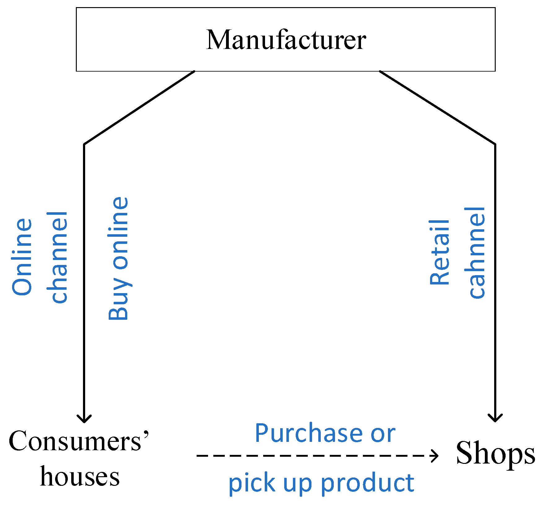
In our models, the omnichannel supply chain is only for one single period and single product. The manufacture supplies the product to retailer and could also sell products for customers through the online channel and BOPS channel. Customers can choose online channel, retail channel or BOPS channel to purchase the product;

(2)

In this model, we assume that customers have the same distance to the pick-up point in store, which means that they are equally sensitive to the price in three channels;

(3)

Substitutability between similar products is not considered in this article;

(4)

The cost of operating the entire omnichannel retail system has not been considered in the profit function;

(5)

Prices of the product in the three channels are not always the same;

(6)

Demand in different channels is affected by product prices in respective channels and the lead time of the online channel;

(7)

The online channel will lose demand when its lead time increases, and some of that demand will transfer to the retail channel and BOPS channel.

3.2. Model Formulation

In this section, we consider the demand in the online channel, retail channel and BOPS channel under the influence of price and lead time, and establish demand formulations. The omnichannel structure of the proposed model is presented in Figure 1. As shown in Figure 1, customers could purchase goods online and wait for goods delivered to their houses, or they can pick up goods in store by themselves. Also, customers can have their whole purchasing process finished at once in physical shops. The deterministic demand in the three channels can be presented as follows:

$$\begin{array}{c} D_o={\lambda }_1-{\alpha }_1{p}_o-{\gamma }_{1}L, \end{array}$$

(1)

$$\begin{array}{c} { D}_r={\lambda }_2-{\alpha }_2{p}_r+{\gamma }_{2}L,\end{array}$$

(2)

$$\begin{array}{c} D_b=\lambda -{\lambda }_1-{\lambda }_2-{\alpha }_3{p}_b+{\gamma }_{3}L,\end{array}$$

(3)

where $D_o$, ${ D}_r$ and $D_b$ represent the demand of online channel, retail channel and BOPS channel, respectively. $\lambda$ represents the total market potential, and the market potential of the product in the online channel, retail channel and BOPS channel can be written as ${\lambda }_1$, ${\lambda }_2$ and $\lambda -{\lambda }_1-{\lambda }_2$, respectively. An increase in product price will lead to a decline in the number of customers. When the delivery lead time $L$ increases, the online channel will lose ${\gamma }_{1}L$ units of demand, while ${\gamma }_{2}L$ units of demand will transfer to the retail channel and ${\gamma }_{3}L$ units of demand will transfer to the BOPS channel.

Now, we consider the randomness in demand, which may cause additional shortage or overstock cost to the total system. Adding an additional part to represent the randomness in demand, the stochastic demand in the online channel, retail channel and BOPS channel can be written as

$$\begin{array}{c} D_{os}={\lambda }_1-{\alpha }_1{p}_o-{\gamma }_{1}L+{\epsilon }_o,\end{array}$$

(4)

$$\begin{array}{c} D_{rs}={\lambda }_2-{\alpha }_2{p}_r+{\gamma }_{2}L+{\epsilon }_r,\end{array}$$

(5)

$$\begin{array}{c} D_{bs}=\lambda -{\lambda }_1-{\lambda }_2-{\alpha }_3{p}_b+{\gamma }_{3}L+{\epsilon }_b,\end{array}$$

(6)

where ${\epsilon }_o$, ${\epsilon }_r$ and ${\epsilon }_b$ are random variables ranging in $[A_o,B_o]$, $[A_r,B_r]$ and $[A_b,B_b]$, with the means of ${\mu }_o$, ${\mu }_r$ and ${\mu }_b$, standard deviations of ${\sigma }_o$, ${\sigma }_r$ and ${\sigma }_b$, and cumulative distribution functions $F_o\left(\cdot \right)$, $F_r\left(\cdot \right)$ and $F_b\left(\cdot \right)$, respectively.

If manufacturers and other members in the supply chain cooperate with each other, all decisions will be made by one decision maker. In this case, products are manufactured in one batch and sold through all three channels. The expected profit function in the supply chain is given by

$$\begin{array}{l}E\left(\pi \right)\\ ={\int }_{A_o}^{z_o}\left[p_o\left(D_o+u_o\right)-h\left(z_o-u_o\right)\right]f_o\left(u_o\right)d{u}_o+{\int }_{z_o}^{B_o}\left[p_o\left(D_o+z_o\right)-\varsigma \left(u_o-z_o\right)\right]f_o\left(u_o\right)d{u}_o\\ +{\int }_{A_r}^{z_r}\left[p_r\left(D_r+u_r\right)-h\left(z_r-u_r\right)\right]f_r\left(u_r\right)d{u}_r+{\int }_{z_r}^{B_r}\left[p_r\left(D_r+z_r\right)-\varsigma \left(u_r-z_r\right)\right]f_r\left(u_r\right)d{u}_r \\ +{\int }_{A_b}^{z_b}\left[p_b\left(D_b+u_b\right)-h\left(z_b-u_b\right)\right]f_b\left(u_b\right)d{u}_b+{\int }_{z_b}^{B_b}\left[p_b\left(D_b+z_b\right)-\varsigma \left(u_b-z_b\right)\right]f_b\left(u_b\right)d{u}_b\\ -c\left(D_o+z_o\right)-c\left(D_r+z_r\right)-c\left(D_b+z_b\right)-{\left(r_o-r_{1}L\right)}^2 , \end{array}$$

(7)

where $z_o$, $z_r$ and $z_b$ represent the quantity of product ordered and produced for random demand in the online channel, retail channel and BOPS channel, respectively. The first and second terms of the function are the holding cost and the shortage cost in the online channel, respectively. The third and fourth terms are the holding cost and the shortage cost in the retail channel, respectively. The fifth and sixth terms are the holding cost and the shortage cost in the BOPS channel, respectively. The seventh to nineth terms are the production cost of manufacturer. Following [34], the last term ${\left(r_o-r_{1}L\right)}^2$ with $r_o/r_1>L$ is the delivery cost of manufacturer. Simplifying the expression, we have

$$\begin{array}{cc}\hfill E\left(\pi \right)& =\left(p_o-c\right)\left(D_o+{\mu }_o\right)+\left(p_r-c\right)\left(D_r+{\mu }_r\right)+\left(p_b-c\right)\left(D_b+{\mu }_b\right)\hfill \\ & -\left(c+h\right)\left({\Lambda }_o+{\Lambda }_r+{\Lambda }_b\right)-\left(p_o+\varsigma -c\right){\Theta }_o-\left(p_r+\varsigma -c\right){\Theta }_r\hfill \\ & -\left(p_b+\varsigma -c\right){\Theta }_b-{\left(r_0-r_{1}L\right)}^2,\hfill \end{array}$$

(8)

where ${\Lambda }_o={\int }_{A_o}^{z_o}\left(z_o-u\right)f_o\left(u\right)du$, ${\Lambda }_r={\int }_{A_r}^{z_r}\left(z_r-u\right)f_r\left(u\right)du$ and ${\Lambda }_b={\int }_{A_b}^{z_b}\left(z_b-u\right)f_b\left(u\right)du$ represent the stochastic orders satisfied in the online channel, retail channel and BOPS channel, respectively, and ${\Theta }_o={\int }_{z_o}^{B_o}\left(u-z_o\right)f_o\left(u\right)du$, ${\Theta }_r={\int }_{z_r}^{B_r}\left(u-z_r\right)f_r\left(u\right)du$ and ${\Theta }_b={\int }_{z_b}^{B_b}\left(u-z_b\right)f_b\left(u\right)du$ represent the stochastic orders unsatisfied in the online channel, retail channel and BOPS channel, respectively.

In most cases, due to limited information about the distribution of demand, only the mean and variance of the randomness can be utilized. Using the inequality ${E(D-Q)}^{+}\le \frac{{\left[{\mathsf{\sigma }}^2+{\left(Q-\mu \right)}^2\right]}^{\frac{1}{2}}-\left(Q-\mu \right)}{2}$ in [31], we can maximize the expected profit of the omnichannel system for the worst distribution. For any distribution function of the random variables ${\epsilon }_o$, ${\epsilon }_r$ and ${\epsilon }_b$ with means $\left({\mu }_o,{\mu }_r,{\mu }_b\right)$ and the variances $\left({\sigma }_o^2,{\sigma }_r^2,{\sigma }_b^2\right)$, the minimum expected profit can be expressed as follows:

$$\begin{array}{ll}MinE\left(\pi \right)& =p_o\left(D_o+{\mu }_o\right)+p_r\left(D_r+{\mu }_r\right)+p_b\left(D_b+{\mu }_b\right)-{\left(r_0-r_{1}L\right)}^2\\ & -c\left(D_o+D_r+D_b+z_o+z_r+z_b\right)-h\left(z_o-{\mu }_o\right)-h\left(z_r-{\mu }_r\right)-h\left(z_b-{\mu }_b\right)\\ & -\left(p_o+\varsigma +h\right)\times \frac{{\left[{\sigma }_o^2+{\left(z_o-{\mu }_o\right)}^2\right]}^{\frac{1}{2}}-\left(z_o-{\mu }_o\right)}{2}\\ & -\left(p_r+\varsigma +h\right)\times \frac{{\left[{\sigma }_r^2+{\left(z_r-{\mu }_r\right)}^2\right]}^{\frac{1}{2}}-\left(z_r-{\mu }_r\right)}{2}\\ & -\left(p_b+\varsigma +h\right)\times \frac{{\left[{\sigma }_b^2+{\left(z_b-{\mu }_b\right)}^2\right]}^{\frac{1}{2}}-\left(z_b-{\mu }_b\right)}{2} .\end{array}$$

(9)

The optimization problem under the distribution-free situation can be presented as:

Problem 1

$$\begin{array}{c}\begin{array}{c} \underset{p_o, p_r, p_b, L, z_o, z_r, z_b}{\mathrm{m}\mathrm{a}\mathrm{x}}MinE\left(\pi \right) \\ \mathrm{s}.\mathrm{t}.p_o,p_r,p_b,L,z_o,z_r,z_b>0.\end{array}\end{array}$$

(10)

The model considers seven decision variables jointly. When solving this model under concavity conditions, we can obtain optimal solution to maximize the profit. However, the optimal solution cannot reveal the interactions between different channels and the specific effects of variables on profit. In the following section, we make an effort to analyze the problem more precisely.

4. Effect Analysis on Lead Time and Price

To gain more insights into this supply chain model, we make an effort in this section to analyze the influence of lead time and price to the supply chain, and calculate the optimum value of the seven decision variables in the integrated decision.

4.1. Delivery Lead Time Sensitive Demand

In this section, we first consider the effect of the delivery lead time on the minimum expected profit. Assuming the delivery lead time $L$ to be the only decision variable in the model, we can obtain the optimum value of it to maximize the minimum expected profit $MinE\left(\pi \right)$.

Proposition 1.

For a given set of product prices in three channels ($p_o$, $p_r$, $p_b$) and orders produced to satisfy the random demand ($z_o$, $z_r$, $z_b$), the lower bound of the minimum expected profit $MinE\left(\pi \right)$ can be maximized by implementing an optimal delivery lead time of $L_m^{\mathrm{\ast }}=\frac{2r_0{r}_1-p_o{\gamma }_1+c{\gamma }_1+p_r{\gamma }_2-c{\gamma }_2+p_b{\gamma }_3-c{\gamma }_3}{2r_1^2}$.

Proof. 

From $\frac{dMinE\left(\pi \right)}{dL}=0$, we can obtain

$$L_m^{\ast }=\frac{2r_0{r}_1-p_o{\gamma }_1+c{\gamma }_1+p_r{\gamma }_2-c{\gamma }_2+p_b{\gamma }_3-c{\gamma }_3}{2r_1^2} .$$

In that $\frac{d^{2}MinE\left(\pi \right)}{d{L}^2}=-2r_1^2<0$, $MinE\left(\pi \right)$ is a concave function of $\mathrm{L}$, the maximum value of $MinE\left(\pi \right)$ can be reached when $L=L_m^{\ast }$. □

Furthermore, the delivery lead time $L$ can be influenced by the prices in the three channels, in that $\frac{d{L}_m^{\ast }}{d{p}_o}=\frac{-{\gamma }_1}{2r_1^2}<0$, $\frac{d{L}_m^{\ast }}{d{p}_r}=\frac{{\gamma }_2}{2r_1^2}>0$, $\frac{d{L}_m^{\ast }}{d{p}_b}=\frac{{\gamma }_3}{2r_1^2}>0$. We also notice that $\frac{d{L}_m^{\ast }}{d{\gamma }_1}=\frac{c-p_o}{2r_1^2}<0$, $\frac{d{L}_m^{\ast }}{d{\gamma }_2}=\frac{p_c-c}{2r_1^2}>0$, $\frac{d{L}_m^{\ast }}{d{\gamma }_3}=\frac{p_b-c}{2r_1^2}>0$. The inequalities above show that, in the retail channel and BOPS channel, the optimal value of lead time will increase if the prices of product in the two channels increase, while in the online channel, the optimal value of lead time will decrease if the price of product in the online channel increases. In the retail channel and BOPS channel, the optimal value of lead time will increase if the delivery time sensitivity of product in two channel increases, but the optimal value of lead time will decrease if the delivery time sensitivity of product in the online channel increases.

Excepted $MinE\left(\pi \right)$ is influenced by delivery lead time, the demand for the product is also affected by $L$. Assuming the prices of the product and the cost to the manufacturer are given, we pay attention to the delivery lead time sensitivities ${\gamma }_1$, ${\gamma }_2$ and ${\gamma }_3$ in three channels. Considering Proposition 1, the demand for the product in the online channel, retail channel and BOPS channel can be presented as follows:

$$\begin{array}{c} D_{ol}={\lambda }_1-{\alpha }_1{p}_o+{\mu }_o-{\gamma }_1\cdot \frac{2r_0{r}_1+c{\gamma }_1-p_o{\gamma }_1+p_r{\gamma }_2-c{\gamma }_2+p_b{\gamma }_3-c{\gamma }_3}{2r_1^2} ,\end{array}$$

(11)

$$\begin{array}{c} D_{rl}={\lambda }_2-{\alpha }_2{p}_r+{\mu }_r+{\gamma }_2\cdot \frac{2r_0{r}_1+c{\gamma }_1-p_o{\gamma }_1+p_r{\gamma }_2-c{\gamma }_2+p_b{\gamma }_3-c{\gamma }_3}{2r_1^2} ,\end{array}$$

(12)

$$\begin{array}{c} D_{bl}=\lambda -{\lambda }_1-{\lambda }_2-{\alpha }_3{p}_b+{\mu }_b+{\gamma }_3\cdot \frac{2r_0{r}_1+c{\gamma }_1-p_o{\gamma }_1+p_r{\gamma }_2-c{\gamma }_2+p_b{\gamma }_3-c{\gamma }_3}{2r_1^2}.\end{array}$$

(13)

After taking partial derivatives of the demand function with respect to each of the delivery sensitive parameters ${\gamma }_1$, ${\gamma }_2$ and ${\gamma }_3$, we discovered some interesting results that deserve further discussion. Firstly, we focus on the relationship between the demand for the product and delivery lead time sensitive parameter ${\gamma }_1$.

When ${\gamma }_1$ is the only variable, we can obtain $d{D}_{ol}/d{\gamma }_1=\frac{2{\gamma }_1\left(p_o-c\right)}{2r_1^2}$, $d{D}_{rl}/d{\gamma }_1=\frac{{\gamma }_2\left(c-p_o\right)}{2r_1^2}<0$, ${dD}_{bl}/d{\gamma }_1=\frac{{\gamma }_3\left(c-p_o\right)}{2r_1^2}<0$. As BOPS service always provides extra convenience for consumers [35], we assume that more customers would prefer the BOPS channel rather than the retail channel, namely ${\gamma }_2<{\gamma }_3$. The demand for the product in the three channels changes with ${\gamma }_1$, as is shown in Figure 2. There are five intersection points when the line of $D_{rl}$ and the line of $D_{bl}$ intersect with the curve of $D_{ol}$, and the crossing point of $D_{rl}$ and $D_{bl}$ is above the curve of $D_{ol}$. Comparing $D_{ol}$, $D_{rl}$ and $D_{bl}$, when the demand for the product in the online channel equals that in the BOPS channel, we can obtain the intersection points $x_{1a}$ and $x_{1d}$; when the demand for the product in the online channel equals that in the retail channel, we can obtain the intersection points $x_{1b}$ and $x_{1e}$; when the demand for the product in the BOPS channel equals that in the retail channel, we can obtain the intersection point $x_{1c}$. The five points are calculated and presented as follows:

$$\begin{array}{c} x_{1a}=\frac{\left(p_r-c\right){\gamma }_2+\left(p_b-p_o\right){\gamma }_3+2r_0{r}_1-\sqrt{N_2}}{2\left(p_o-c\right)},\end{array}$$

(14)

$$\begin{array}{c} x_{1b}=\frac{\left(p_r-p_o\right){\gamma }_2+\left(p_b-c\right){\gamma }_3+2r_0{r}_1-\sqrt{N_1}}{2\left(p_o-c\right)},\end{array}$$

(15)

$$\begin{array}{cc}\hfill x_{1c}& =\frac{2r_1^2\left(\lambda -{\lambda }_1-{2\lambda }_2+{\alpha }_2{p}_r-{\alpha }_3{p}_b-{\mu }_r+{\mu }_b\right)}{\left(c-p_o\right)\left({\gamma }_2-{\gamma }_3\right)}\hfill \\ & +\frac{\left({\gamma }_3-{\gamma }_2\right)\left[2r_0{r}_1+\left(p_r-c\right){\gamma }_2+\left(p_b-c\right){\gamma }_3\right]}{\left(c-p_o\right)\left({\gamma }_2-{\gamma }_3\right)},\hfill \end{array}$$

(16)

$$\begin{array}{c} x_{1d}=\frac{\left(p_r-p_o\right){\gamma }_2+\left(p_b-c\right){\gamma }_3+2r_0{r}_1+\sqrt{N_1}}{2\left(p_o-c\right)},\end{array}$$

(17)

$$\begin{array}{c} x_{1e}=\frac{\left(p_r-c\right){\gamma }_2+\left(p_b-p_o\right){\gamma }_3+2r_0{r}_1+\sqrt{N_2}}{2\left(p_o-c\right)},\end{array}$$

(18)

where $N_1={\left[\left(p_o-p_r\right){\gamma }_2-\left(p_b-c\right){\gamma }_3-2r_0{r}_1\right]}^2+4\left(c-p_o\right)[2r_1^2\left({\lambda }_1-{\lambda }_2-{\alpha }_1{p}_o+{\alpha }_2{p}_r+{\mu }_o-{\mu }_r\right)-{\gamma }_2[\left(p_r-c\right){\gamma }_2+\left(p_b-c\right){\gamma }_3+2r_0{r}_1\left]\right]$, $$\begin{gathered} N_2={\left[\left(p_r-c\right){\gamma }_2+\left(p_b-p_o\right){\gamma }_3+2r_0{r}_1\right]}^2 \\ +4\left(c-p_o\right)[2r_1^2\left(2{\lambda }_1+{\lambda }_2-\lambda -{\alpha }_1{p}_o+{\alpha }_3{p}_b+{\mu }_o-{\mu }_b\right)-{\gamma }_3[\left(p_r-c\right){\gamma }_2+\left(p_b-c\right){\gamma }_3+2r_0{r}_1\left]\right]. \end{gathered}$$

According to its definition, the sensitive parameter of delivery lead time is greater than $0$, so we are only concerned with the situation where ${\gamma }_1>0$. In the figures below, the portion where ${\gamma }_1<0$ is covered by blue rectangle, meaning that is not contained in our discussion. Combined with the figure which has five intersection points in Figure 2 and the analyses upon this, we obtain the following conclusions. If $max\left(0,x_{1b}\right)<{\gamma }_1<x_{1c}$, then $D_{ol}<D_{rl}<D_{bl}$. If $x_{1c}<{\gamma }_1<x_{1d}$, then $D_{ol}<D_{bl}<D_{rl}$. If $x_{1d}<{\gamma }_1<x_{1e}$, then $D_{bl}<D_{ol}<D_{rl}$. If ${\gamma }_1>x_{1e}$, then $D_{bl}<D_{rl}<D_{ol}$.

Unlike the figure which has five intersection points, the distribution and intersections of the demand lines and curve can be changed in different situations. If the demand lines of the retail channel and BOPS channel have no crossing point when ${\gamma }_1>0$, there are only four intersection points in the figure. Combined with the figure which has four intersection points, we can conclude that if $max\left(0,x_{1a}\right)<{\gamma }_1<x_{1d}$, then $D_{ol}<D_{bl}<D_{rl}$. If $x_{1d}<{\gamma }_1<x_{1e}$, $D_{bl}<D_{ol}<D_{rl}$. If ${\gamma }_1{>x}_{1e}$, $D_{bl}<D_{rl}<D_{ol}$.

There are two situations in which the figure has three intersection points. The first occurs when the lines of $D_{rl}$, $D_{bl}$ and $D_{ol}$ intersect at one point on the left. In this situation, if $\max (0,x_{1c})<{\gamma }_1<x_{1d}$, then $D_{ol}<D_{bl}<D_{rl}$. If $x_{1d}<{\gamma }_1<x_{1e}$, then $D_{bl}<D_{ol}<D_{rl}$. If ${\gamma }_1{>x}_{1e}$, then $D_{bl}<D_{rl}<D_{ol}$. Another situation occurs when the lines of $D_{rl}$, $D_{bl}$ and $D_{ol}$ intersect at one point on the right side. In this situation, if $\max (0,x_{1b})<{\gamma }_1<x_{1c}$, then $D_{ol}<D_{rl}<D_{bl}$. If ${\gamma }_1{>x}_{1c}$, then $D_{bl}<D_{rl}<D_{ol}$.

Now, we mainly consider the influence delivery sensitive parameter ${\gamma }_2$ made to the demand for the product. When ${\gamma }_2$ is the only variable, we can obtain $d{D}_{ol}/d{\gamma }_2=\frac{{-\gamma }_1\left(p_r-c\right)}{2r_1^2}<0$, $d{D}_{rl}/d{\gamma }_2=\frac{{2\gamma }_2\left(p_r-c\right)}{2r_1^2}$, ${dD}_{bl}/d{\gamma }_2=\frac{{\gamma }_3\left(p_r-c\right)}{2r_1^2}>0$. It is obvious that $D_{rl}$ is a convex function of ${\gamma }_2$, and the slope of $D_{ol}$ and $D_{bl}$ with respect to ${\gamma }_2$ is negative and positive, respectively (see Figure 3). There are five intersection points when the line of $D_{ol}$ and the line of $D_{bl}$ intersect with the curve of $D_{rl}$, and the crossing point of $D_{ol}$ and $D_{bl}$ is above the curve of $D_{rl}$. Comparing $D_{ol}$, $D_{rl}$ and $D_{bl}$, when the demand for the product in the online channel equals that in the retail channel, we can obtain the intersection points $x_{2a}$ and $x_{2d}$; when the demand for the product in the BOPS channel equals that in the retail channel, we can obtain the intersection points $x_{2b}$ and $x_{2e}$; when the demand for the product in the online channel equals that in the BOPS channel, we can obtain the intersection point $x_{2c}$. We calculate the five points and present them as follows:

$$\begin{array}{c} x_{2a}=\frac{-2r_0{r}_1+\left(p_o-p_r\right){\gamma }_1-\left(p_b-c\right){\gamma }_3-\sqrt{N_3}}{2\left(p_r-c\right)},\end{array}$$

(19)

$$\begin{array}{c} x_{2b}=\frac{-2r_0{r}_1+\left(p_o-c\right){\gamma }_1-\left(p_b-p_r\right){\gamma }_3-\sqrt{N_4}}{2\left(p_r-c\right)}, \end{array}$$

(20)

$$\begin{array}{cc}\hfill x_{2c}& =\frac{2r_1^2\left(2{\lambda }_1+{\lambda }_2-\lambda -{\alpha }_1{p}_o+{\alpha }_3{p}_b+{\mu }_o-{\mu }_b\right)}{\left(p_r-c\right)\left({\gamma }_1+{\gamma }_3\right)}\hfill \\ & -\frac{\left({\gamma }_1+{\gamma }_3\right)\left[2r_0{r}_1+\left(p_r-c\right){\gamma }_2+\left(p_b-c\right){\gamma }_3\right]}{\left(p_r-c\right)\left({\gamma }_1+{\gamma }_3\right)},\hfill \end{array}$$

(21)

$$\begin{array}{c} x_{2d}=\frac{-2r_0{r}_1+\left(p_o-p_r\right){\gamma }_1-\left(p_b-c\right){\gamma }_3+\sqrt{N_3}}{2\left(p_r-c\right)},\end{array}$$

(22)

$$\begin{array}{c} x_{2e}=\frac{-2r_0{r}_1+\left(p_o-c\right){\gamma }_1-\left(p_b-p_r\right){\gamma }_3+\sqrt{N_4}}{2\left(p_r-c\right)},\end{array}$$

(23)

where $N_3={\left[\left(p_r-p_o\right){\gamma }_1+\left(p_b-c\right){\gamma }_3+2r_0{r}_1\right]}^2+4\left(p_r-c\right)[2r_1^2\left({\lambda }_1-{\lambda }_2-{\alpha }_1{p}_o+{\alpha }_2{p}_r+{\mu }_o-{\mu }_r\right)-{\gamma }_1[-\left(p_o-c\right){\gamma }_1+\left(p_b-c\right){\gamma }_3+2r_0{r}_1\left]\right]$, $$\begin{gathered} N_4={\left[\left(p_o-c\right){\gamma }_1-\left(p_b-p_r\right){\gamma }_3-2r_0{r}_1\right]}^2 \\ +4\left(p_r-c\right)[2r_1^2\left(\lambda -{\lambda }_1-2{\lambda }_2+{\alpha }_2{p}_r-{\alpha }_3{p}_b+{\mu }_b-{\mu }_r\right)+{\gamma }_3[-\left(p_o-c\right){\gamma }_1+\left(p_b-c\right){\gamma }_3+2r_0{r}_1\left]\right]. \end{gathered}$$

Since ${\gamma }_2>0$, we focus on the portion which is not covered by the blue rectangle. According to Figure 3, there are three situations. From the figure which has five intersection points, we can see that if ${\gamma }_2>max\left(0,x_{2e}\right)$, then $D_{ol}<D_{bl}<D_{rl}$. There are two situations when the figure has three intersection points. The first situation occurs when the lines of $D_{ol}$, $D_{bl}$ and $D_{rl}$ intersect at one point on the left. In this situation, if $x_{2d}<{\gamma }_2<x_{2e}$, then $D_{ol}<D_{rl}<D_{bl}$. If ${\gamma }_2>x_{2e}$, then $D_{ol}<D_{bl}<D_{rl}$. The second situation occurs when the lines of $D_{ol}$, $D_{bl}$ and $D_{rl}$ intersect at one point on the right. In this situation, if $max\left(0,x_{2b}\right)<{\gamma }_2<x_{2c}$, then $D_{rl}<D_{bl}<D_{ol}$. If ${\gamma }_2>x_{2c}$, then $D_{ol}<D_{bl}<D_{rl}$.

To the last sensitive parameter of delivery ${\gamma }_3$, we also obtain some conclusions. When ${\gamma }_3$ is the only variable, we can obtain $d{D}_{ol}/d{\gamma }_3=\frac{{-\gamma }_1\left(p_b-c\right)}{2r_1^2}<0$, $d{D}_{rl}/d{\gamma }_3=\frac{{\gamma }_2\left(p_b-c\right)}{2r_1^2}>0$, ${dD}_{bl}/d{\gamma }_3=\frac{{2\gamma }_3\left(p_b-c\right)}{2r_1^2}$. It is obvious that $D_{bl}$ is a convex function of ${\gamma }_3$, and $D_{ol}$ and $D_{rl}$ have negative and positive slopes with respect to ${\gamma }_3$, respectively (see Figure 4). There are five intersection points in the figure when the line of $D_{ol}$ and the line of $D_{rl}$ intersect with the curve of $D_{bl}$, and the crossing point of $D_{ol}$ and $D_{rl}$ is above the curve of $D_{bl}$. Comparing $D_{ol}$, $D_{rl}$ and $D_{bl}$, when the demand for the product in the online channel equals that in the BOPS channel, we can obtain the intersection points $x_{3a}$ and $x_{3d}$; when the demand for the product in the retail channel equals that in the BOPS channel, we can obtain the intersection points $x_{3b}$ and $x_{3e}$; when the demand for the product in the online channel equals that in the retail channel, we can obtain the intersection point $x_{3c}$. We calculate the five points and present them as follows:

$$\begin{array}{c} x_{3a}=\frac{-2r_0{r}_1+\left(p_o-p_b\right){\gamma }_1-\left(p_r-c\right){\gamma }_3-\sqrt{N_5}}{2\left(p_b-c\right)},\end{array}$$

(24)

$$\begin{array}{c} x_{3b}=\frac{-2r_0{r}_1+\left(p_o-c\right){\gamma }_1+\left(p_b-p_r\right){\gamma }_2-\sqrt{N_6}}{2\left(p_b-c\right)},\end{array}$$

(25)

$$\begin{array}{cc}\hfill x_{3c}& =\frac{2r_1^2\left({\lambda }_1-{\lambda }_2-{\alpha }_1{p}_o+{\alpha }_2{p}_r+{\mu }_o-{\mu }_r\right)}{\left(p_b-c\right)\left({\gamma }_1+{\gamma }_2\right)}\hfill \\ & -\frac{\left({\gamma }_1+{\gamma }_2\right)\left[2r_0{r}_1+\left(c-p_o\right){\gamma }_1+\left(p_r-c\right){\gamma }_2\right]}{\left(p_b-c\right)\left({\gamma }_1+{\gamma }_2\right)},\hfill \end{array}$$

(26)

$$\begin{array}{c} x_{3d}=\frac{-2r_0{r}_1+\left(p_o-p_b\right){\gamma }_1-\left(p_r-c\right){\gamma }_3+\sqrt{N_5}}{2\left(p_b-c\right)},\end{array}$$

(27)

$$\begin{array}{c} x_{3e}=\frac{-2r_0{r}_1+\left(p_o-c\right){\gamma }_1+\left(p_b-p_r\right){\gamma }_2+\sqrt{N_6}}{2\left(p_b-c\right)},\end{array}$$

(28)

where $N_5={\left[\left(p_b-p_o\right){\gamma }_1+\left(p_r-c\right){\gamma }_2+2r_0{r}_1\right]}^2+4\left(p_b-c\right)[2r_1^2\left(2{\lambda }_1+{\lambda }_2-\lambda -{\alpha }_1{p}_o+{\alpha }_3{p}_b+{\mu }_o-{\mu }_b\right)-{\gamma }_1[-\left(p_o-c\right){\gamma }_1+\left(p_r-c\right){\gamma }_2+2r_0{r}_1\left]\right]$, $N_6={\left[\left(p_o-c\right){\gamma }_1+\left(p_b-p_r\right){\gamma }_2-2r_0{r}_1\right]}^2+4\left(p_b-c\right)[2r_1^2\left(2{\lambda }_2+{\lambda }_1-\lambda -{\alpha }_2{p}_r+{\alpha }_3{p}_b+{\mu }_r-{\mu }_b\right)+{\gamma }_2[-\left(p_o-c\right){\gamma }_1+\left(p_r-c\right){\gamma }_2+2r_0{r}_1\left]\right]$.

Since the sensitive parameter of delivery lead time is defined as greater than $0$, we only focus on the situation where ${\gamma }_3$ is greater than 0. In the figure which has five intersection points, we can see that if $x_{3d}<{\gamma }_3<x_{3e}$, then $D_{ol}<D_{bl}<D_{rl}$. If ${\gamma }_3{>x}_{3e}$, then $D_{ol}<D_{rl}<D_{bl}$. There are two situations when the figure has three intersection points. The first situation occurs when the lines of $D_{ol}$, $D_{rl}$ and $D_{bl}$ intersect at one point on the left. In this situation, if $x_{3d}<{\gamma }_3<x_{3e}$, we have $D_{ol}<D_{bl}<D_{rl}$. If ${\gamma }_3{>x}_{3e}$, then $D_{ol}<D_{rl}<D_{bl}$. The second situation occurs when the lines of $D_{ol}$, $D_{rl}$ and $D_{bl}$ intersect at one point on the right. In this situation, if ${\gamma }_3{>x}_{3c}$, then $D_{ol}<D_{rl}<D_{bl}$.

From the analyses above, we can obtain a deep insight into the relationship between delivery lead time sensitivity and demand for the product in different channels. As the delivery lead time sensitivity changes, the demand comparisons across the three channels will be different. The intersection points to different situations playing a key role in predicting demand trend, which are critical when making decisions.

4.2. Price Sensitive Demand

In this section, we take product price into consideration. We first examine the influence of price on the minimum expected profit and then consider the relationship between price and lead time. When order quantities ($z_o$, $z_r$, $z_b$) and delivery lead time ($L$) are given, we can obtain the optimum price to maximize the minimum expected profit $MinE\left(\pi \right)$.

Proposition 2.

For given $z_o$, $z_r$, $z_b$, $L$, the minimum expected profit function, $MinE\left(\pi \right)$, can reach its optimum value when the prices of product in the online channel, retail channel and BOPS channel are set as follows:

$$\begin{array}{c} p_{om}^{\ast }=\frac{2{\lambda }_1-2{\gamma }_{1}L+2{\mu }_o+2c{\alpha }_1-{\left[{\sigma }_o^2+{\left(z_o-{\mu }_o\right)}^2\right]}^{\frac{1}{2}}+\left(z_o-{\mu }_o\right) }{4{\alpha }_1} ,\end{array}$$

(29)

$$\begin{array}{c} p_{rm}^{\ast }=\frac{2{\lambda }_2+2{\gamma }_{2}L+2{\mu }_r+2c{\alpha }_2-{\left[{\sigma }_r^2+{\left(z_r-{\mu }_r\right)}^2\right]}^{\frac{1}{2}}+\left(z_r-{\mu }_r\right)}{4{\alpha }_2} , \end{array}$$

(30)

$$\begin{array}{c} p_{bm}^{\ast }=\frac{2\lambda -2{\lambda }_1-2{\lambda }_2+2{\gamma }_{3}L+2{\mu }_b+2c{\alpha }_3-{\left[{\sigma }_b^2+{\left(z_b-{\mu }_b\right)}^2\right]}^{\frac{1}{2}}+\left(z_b-{\mu }_b\right)}{4{\alpha }_3} . \end{array}$$

(31)

Proof. 

From $dMinE\left(\pi \right)/d{p}_o=0$, $dMinE\left(\pi \right)/d{p}_r=0$, $dMinE\left(\pi \right)/d{p}_b=0$, we can obtain

$$p_o=\frac{2{\lambda }_1-2{\gamma }_{1}L+2{\mu }_o+2c{\alpha }_1-{\left[{\sigma }_o^2+{\left(z_o-{\mu }_o\right)}^2\right]}^{\frac{1}{2}}+\left(z_o-{\mu }_o\right) }{4{\alpha }_1} ,$$

$$p_r=\frac{2{\lambda }_2+2{\gamma }_{2}L+2{\mu }_r+2c{\alpha }_2-{\left[{\sigma }_r^2+{\left(z_r-{\mu }_r\right)}^2\right]}^{\frac{1}{2}}+\left(z_r-{\mu }_r\right)}{4{\alpha }_2} ,$$

$$p_b=\frac{2\lambda -2{\lambda }_1-2{\lambda }_2+2{\gamma }_{3}L+2{\mu }_b+2c{\alpha }_3-{\left[{\sigma }_b^2+{\left(z_b-{\mu }_b\right)}^2\right]}^{\frac{1}{2}}+\left(z_b-{\mu }_b\right)}{4{\alpha }_3} .$$

We also see that $\frac{d^{2}MinE\left(\pi \right)}{d{p_o}^2}=-2{\alpha }_1<0$, $\frac{d^{2}MinE\left(\pi \right)}{d{p_r}^2}=-2{\alpha }_2<0$, $\frac{d^{2}MinE\left(\pi \right)}{d{p_b}^2}=-2{\alpha }_3<0$, so $MinE\left(\pi \right)$ is a concave function of $p_o$, $p_r$ and $p_b$. Hence, when $p_o$, $p_r$ and $p_b$ are set, satisfying $dMinE\left(\pi \right)/d{p}_o=0$, $dMinE\left(\pi \right)/d{p}_r=0$, and $dMinE\left(\pi \right)/d{p}_b=0$, $MinE\left(\pi \right)$ will reach its optimum value. □

We also notice that $d{p}_{om}^{\ast }/dL=-{\gamma }_1/2{\alpha }_1$, $d{p}_{rm}^{\ast }/dL={\gamma }_2/2{\alpha }_2$, $d{p}_{bm}^{\ast }/dL={\gamma }_3/2{\alpha }_3$. Since the sensitive parameters ${\gamma }_1$, ${\gamma }_2$, ${\gamma }_3$ of lead time $L$ and prices are all positive in three channels, we can see that $d{p}_{om}^{\ast }/dL<0$, $d{p}_{rm}^{\ast }/dL>0$, $d{p}_{bm}^{\ast }/dL>0$, which reveals that only the price of the product in the online channel will decrease with the rising lead time, while the prices of products in the retail channel and BOPS channel will increase with the rising lead time. Furthermore, if ${\gamma }_2/2{\alpha }_2-{\gamma }_3/2{\alpha }_3>0$ (${\gamma }_2/2{\alpha }_2-{\gamma }_3/2{\alpha }_3<0$), the rate of increment of price is higher (lower) in the retail channel than in the BOPS channel. With the lead time sensitivity parameter ${\gamma }_1$, we have $\frac{d{p}_{om}^{\ast }}{d{\gamma }_1}=-\frac{L}{2{\alpha }_1}<0$, which shows that $p_{om}^{\ast }$ will decrease as ${\gamma }_1$ increases. With the lead time sensitivity parameter ${\gamma }_2$ and ${\gamma }_3$, it is easy to obtain $\frac{d{p}_{rm}^{\ast }}{d{\gamma }_2}=\frac{L}{2{\alpha }_2}>0$ and $\frac{d{p}_{bm}^{\ast }}{d{\gamma }_3}=\frac{L}{2{\alpha }_3}>0$, which show that $p_{rm}^{\ast }$ and $p_{bm}^{\ast }$ will increase when ${\gamma }_2$ and ${\gamma }_3$ increase. When ${\alpha }_2>{\alpha }_3$ (${\alpha }_2<{\alpha }_3$), the rate of increment of price is higher (lower) in the retail channel than in the BOPS channel.

4.3. Decision Variables in the Integrated Decision

The analyses above consider the optimum value of decision variables separately, to maximize the minimum expected profit when the distribution of demand is unknown. For given distribution functions $F_o\left(\cdot \right)$, $F_r\left(\cdot \right)$ and $F_b\left(\cdot \right)$ of the random variables ${\epsilon }_o$, ${\epsilon }_r$ and ${\epsilon }_b$, we take the decision variables into account simultaneously and obtain the proposition below.

Proposition 3.

When the distribution of random demand  ${\epsilon }_o$,  ${\epsilon }_r$,  ${\epsilon }_b$ are known, the expected profit function $E\left(\pi \right)$ can reach its optimum value, if $p_o$, $p_r$, $p_b$, $L$, $z_o$, $z_r$, $z_b$ are set as follows:

$$\begin{array}{c} z_o^{\ast }={F_o}^{-1}\left(\frac{p_o+\varsigma -c}{p_o+\varsigma +h}\right), \end{array}$$

(32)

$$\begin{array}{c} z_r^{\ast }={F_r}^{-1}\left(\frac{p_r+\varsigma -c}{p_r+\varsigma +h}\right),\end{array}$$

(33)

$$\begin{array}{c} z_b^{\ast }={F_b}^{-1}\left(\frac{p_b+\varsigma -c}{p_b+\varsigma +h}\right),\end{array}$$

(34)

$$\begin{array}{c} p_o^{\ast }=\frac{{\lambda }_1-{\gamma }_{1}L+{\mu }_o+c{\alpha }_1-{\Theta }_o^{\ast }}{2{\alpha }_1} ,\end{array}$$

(35)

$$\begin{array}{c} p_r^{\ast }=\frac{{\lambda }_2+{\gamma }_{2}L+{\mu }_r+c{\alpha }_2-{\Theta }_r^{\ast }}{2{\alpha }_2} ,\end{array}$$

(36)

$$\begin{array}{c} p_b^{\ast }=\frac{\lambda -{\lambda }_1-{\lambda }_2+{\gamma }_{3}L+{\mu }_b+c{\alpha }_3-{\Theta }_b^{\ast }}{2{\alpha }_3} ,\end{array}$$

(37)

$$\begin{array}{c}\begin{array}{c}{L}^{\ast }=\frac{{\gamma }_1\left[{\lambda }_1-{\gamma }_{1}L+{\mu }_o+c{\alpha }_1-{\Theta }_o^{\ast }\right]-c{\gamma }_1}{2{\alpha }_1{r}_1}+\frac{{\gamma }_2\left[{\lambda }_2+{\gamma }_{2}L+{\mu }_r+c{\alpha }_2-{\Theta }_r^{\ast }\right]-c{\gamma }_2}{2{\alpha }_2{r}_1}\\ +\frac{{\gamma }_3\left[\lambda -{\lambda }_1-{\lambda }_2+{\gamma }_{3}L+{\mu }_b+c{\alpha }_3-{\Theta }_b^{\ast }\right]-c{\gamma }_3}{2{\alpha }_3{r}_1}+2r_0 , \end{array}\end{array}$$

(38)

where ${\Theta }_o^{\ast }={\int }_{z_{\mathrm{o}}^{\ast }}^{B_o}\left(u-z_{\mathrm{o}}^{\ast }\right)f_o\left(u\right)du$, ${\Theta }_r^{\ast }={\int }_{z_{\mathrm{r}}^{\ast }}^{B_o}\left(u-z_{\mathrm{r}}^{\ast }\right)f_r\left(u\right)du$, ${\Theta }_b^{\ast }={\int }_{z_b^{\ast }}^{B_o}\left(u-z_{\mathrm{b}}^{\ast }\right)f_b\left(u\right)du$; ${\Lambda }_{\mathrm{o}}^{\ast }={\int }_{A_o}^{z_{\mathrm{o}}^{\ast }}\left(z_{\mathrm{o}}^{\ast }-u\right)f_o\left(u\right)du$, ${\Lambda }_{\mathrm{r}}^{\ast }={\int }_{A_r}^{z_{\mathrm{r}}^{\ast }}\left(z_{\mathrm{r}}^{\ast }-u\right)f_r\left(u\right)du$ and ${\Lambda }_{\mathrm{b}}^{\ast }={\int }_{A_b}^{z_b^{\ast }}\left(z_{\mathrm{b}}^{\ast }-u\right)f_b\left(u\right)du$.

Proof. 

When random variables ${\epsilon }_o$, ${\epsilon }_r$, ${\epsilon }_b$ have known distribution functions $F_o\left(\cdot \right)$, $F_r\left(\cdot \right)$ and $F_b\left(\cdot \right)$, by using KKT conditions in the supply channel, we have

$$\frac{\mathsf{\partial }E\left(\pi \right)}{\mathsf{\partial }{z}_o}=-\left(c+h\right)F_o\left(z_o\right)+\left(p_o+\varsigma -c\right)\left(1-F_o\left(z_o\right)\right)=0 ,$$

$$\frac{\mathsf{\partial }E\left(\pi \right)}{\mathsf{\partial }{z}_r}=-\left(c+h\right)F_r\left(z_r\right)+\left(p_r+\varsigma -c\right)\left(1-F_r\left(z_r\right)\right)=0 ,$$

$$\frac{\mathsf{\partial }E\left(\pi \right)}{\mathsf{\partial }{z}_b}=-\left(c+h\right)F_b\left(z_b\right)+\left(p_b+\varsigma -c\right)\left(1-F_b\left(z_b\right)\right)=0 ,$$

$$\frac{\mathsf{\partial }E\left(\pi \right)}{\mathsf{\partial }{p}_o}={\lambda }_1-2{\alpha }_1{p}_o-{\gamma }_{1}L+{\mu }_o+c{\alpha }_1-{\Theta }_o=0 ,$$

$$\frac{\mathsf{\partial }E\left(\pi \right)}{\mathsf{\partial }{p}_r}={\lambda }_2-2{\alpha }_2{p}_r+{\gamma }_{2}L+{\mu }_r+c{\alpha }_2-{\Theta }_r=0 ,$$

$$\frac{\mathsf{\partial }E\left(\pi \right)}{\mathsf{\partial }{p}_b}=\lambda -{\lambda }_1-{\lambda }_2-2{\alpha }_3{p}_b+{\gamma }_{3}L+{\mu }_b+c{\alpha }_3-{\Theta }_b=0 ,$$

$$\frac{\mathsf{\partial }E\left(\pi \right)}{\mathsf{\partial }L}=\left(p_o-c\right){\gamma }_1+\left(p_r-c\right){\gamma }_2+\left(p_b-c\right){\gamma }_3+2r_1\left(r_0-r_{1}L\right)=0 .$$

By solving the functions above simultaneously, we can obtain the value of $p_o^{\ast }$, $p_r^{\ast }$, $p_b^{\ast }$, $L^{\ast }$, $z_o^{\ast }$, $z_r^{\ast }$, $z_b^{\ast }$. With the optimal values of the seven decision variables, the expected profit function, $E\left(\pi \right)$, will obtain its optimum value if its Hessian matrix is negative definite. □

5. Numerical Illustration

In this part, we assume the demand is normally distributed. We set ${\lambda }_1=150$, ${\lambda }_2=120$, $\lambda =390$, then the market potential of demand in three channels are 150, 120, 120, respectively. $c=50$, $s=30$, $h=3$, $r_0=70$, $r_1=7$, ${\alpha }_1=0.75$, ${\alpha }_2=0.8$, ${\alpha }_3=0.7$, ${\gamma }_1=0.7$, ${\gamma }_2=0.2$, ${\gamma }_3=0.3$. We assume that the random variables ${\epsilon }_o$, ${\epsilon }_r$ and ${\epsilon }_b$ are distributed normally on the ranges [–50, 100], [−40, 95] and [−30, 80], with the means ${\mu }_o=25$, ${\mu }_r=30$ and ${\mu }_b=28$, respectively, and the standard deviations are ${\sigma }_o=4$, ${\sigma }_r=5$, ${\sigma }_b=4$, respectively. The Hessian matrix of the minimum expected profit function is

$$Mmin=\left[\begin{array}{ccc}-1.5& \begin{array}{ccc}0& 0& -0.7\end{array}& \begin{array}{ccc}0& 0 & 0\end{array}\\ \begin{array}{c}0\\ 0\\ -0.7\end{array}& \begin{array}{ccc}-1.6& 0& 0.2\\ 0& -1.4& 0.3\\ 0.2& 0.3& -98\end{array}& \begin{array}{ccc}0& 0& 0\\ 0& 0& 0\\ 0& 0& 0\end{array}\\ \begin{array}{c}0\\ 0\\ 0\end{array}& \begin{array}{ccc}0& 0& 0\\ 0& 0& 0\\ 0& 0& 0\end{array}& \begin{array}{ccc}-13.7383& 0& 0\\ 0& -18.2474& 0\\ 0& 0& -13.1113\end{array}\end{array}\right]$$

The eigenvalues of the matrix are $(-98.0064;-18.2474;-13.7383;-13.1113;-1.5996;-1.4950;-1.3990)$. As the eigenvalues of Hessian matrix are all negative, $Mmin$ is negative definite and the minimum expected profit function has local maximum value. The optimal values of decision variables are as follows: $z_o^{\ast }=26.9535, z_r^{\ast }=31.9791, z_b^{\ast }=29.8804,{ L}^{\ast }=11.0155, p_o^{\ast }=136.5247,p_r^{\ast }=120.1263,$ $p_b^{\ast }=133.0726.$ The minimum expected profit is 12847.

When other parameters and delivery sensitive parameters in the online channel are constant, but the number of consumers who leave the online channel due to unexpected lead time and choose to turn to retail channel and BOPS channel decrease, the minimum expected profit will decrease, the decision variables will be affected as well (see

Table 1. Optimal values of decision variables with different ${\gamma }_i ({\gamma }_1=0.7)$.

${\mathit{\gamma }}_{\mathit{i}}$	${\mathit{\gamma }}_2=0.2$ ${\mathit{\gamma }}_3=0.3$	${\mathit{\gamma }}_2=0.2$ ${\mathit{\gamma }}_3=0.2$	${\mathit{\gamma }}_2=0.1$ ${\mathit{\gamma }}_3=0.2$	${\mathit{\gamma }}_2=0.1$ ${\mathit{\gamma }}_3=0.1$
$z_o^{\ast }$	$26.9535$	26.9544	26.9551	26.9559
$z_r^{\ast }$	$31.9791$	31.9788	31.9576	31.9575
$z_b^{\ast }$	$29.8804$	29.8632	29.8630	29.8459
${ L}^{\ast }$	$11.0155$	10.9293	10.8573	10.7728
$p_o^{\ast }$	$136.5247$	136.5649	136.5985	136.6379
$p_r^{\ast }$	$120.1263$	120.1155	119.4279	119.4226
$p_b^{\ast }$	$133.0726$	132.2734	132.2631	131.4814
$MinE\left(\pi \right)$	$12847$	12766	12679	12600

).

The growth of the mean of random variables ${\mu }_a(a=o,r,b)$ and standard deviations ${\sigma }_a(a=o,r,b)$ have different effects on the minimum expected profit (see

Table 2. Optimal values of decision variables with different ${\mu }_a(a=o,r,b)$.

	${\mathit{\mu }}_{\mathit{o}}=5$ ${\mathit{\mu }}_{\mathit{r}}=5$ ${\mathit{\mu }}_{\mathit{b}}=5$	${\mathit{\mu }}_{\mathit{o}}=30$ ${\mathit{\mu }}_{\mathit{r}}=5$ ${\mathit{\mu }}_{\mathit{b}}=5$	${\mathit{\mu }}_{\mathit{o}}=30$ ${\mathit{\mu }}_{\mathit{r}}=30$ ${\mathit{\mu }}_{\mathit{b}}=5$	${\mathit{\mu }}_{\mathit{o}}=30$ ${\mathit{\mu }}_{\mathit{r}}=30$ ${\mathit{\mu }}_{\mathit{b}}=30$
$z_o^{\ast }$	6.6612	32.0243	32.0242	32.0240
$z_r^{\ast }$	6.4296	6.4299	31.9575	31.9575
$z_b^{\ast }$	6.4550	6.4553	6.4553	31.8770
${ L}^{\ast }$	10.6453	10.7639	10.7798	10.7980
$p_o^{\ast }$	123.3612	139.9757	139.9683	139.9598
$p_r^{\ast }$	103.7860	103.7934	119.4230	119.4242
$p_b^{\ast }$	115.0371	115.0456	115.0467	132.9120
$MinE\left(\pi \right)$	7790.7	9297.5	11275	13097

and

Table 3. Optimal values of decision variables with different ${\sigma }_a(a=o,r,b)$.

	${\mathit{\sigma }}_{\mathit{o}}=1.5$ ${\mathit{\sigma }}_{\mathit{r}}=1.5$ ${\mathit{\sigma }}_{\mathit{b}}=1.5$	${\mathit{\sigma }}_{\mathit{o}}=4$ ${\mathit{\sigma }}_{\mathit{r}}=1.5$ ${\mathit{\sigma }}_{\mathit{b}}=1.5$	${\mathit{\sigma }}_{\mathit{o}}=4$ ${\mathit{\sigma }}_{\mathit{r}}=5$ ${\mathit{\sigma }}_{\mathit{b}}=1.5$	${\mathit{\sigma }}_{\mathit{o}}=4$ ${\mathit{\sigma }}_{\mathit{r}}=5$ ${\mathit{\sigma }}_{\mathit{b}}=4$
$z_o^{\ast }$	25.7275	26.9559	26.9559	$26.9535$
$z_r^{\ast }$	30.5791	30.5791	31.9574	$31.9791$
$z_b^{\ast }$	28.6850	28.6850	28.6850	$29.8804$
${ L}^{\ast }$	10.7656	10.7710	10.7719	$11.0155$
$p_o^{\ast }$	135.8795	136.6387	136.6383	$136.5247$
$p_r^{\ast }$	118.5502	118.5506	119.4226	$120.1263$
$p_b^{\ast }$	130.5975	130.5979	130.5980	$133.0726$
$MinE\left(\pi \right)$	13242	13021	12793	$12847$

). When other parameters are constant, the minimum expected profit $MinE\left(\pi \right)$ will increase with the rise of the mean of random variables ${\mu }_a(a=o,r,b)$, since the total consumers are increased, while $MinE\left(\pi \right)$ will decrease with an increase in standard deviations ${\sigma }_a(a=o,r,b)$ as the manufacture will undertake more cost in inventory.

5.1. Sensitivity Analysis

To further investigate the impact of parameters on the optimal decision and total profit, a sensitivity analysis is conducted in this section with changing unit holding cost $h$, unit cost of manufacturer $c$, delivery-time-dependent cost parameters $r_0$ and $r_1$, price sensitivity ${\alpha }_i(i=1,2,3)$ and market potential ${\lambda }_i(i=1,2,3)$. Compared to the base case, we examine the variance of the optimum solution and the minimum expected profit value when $h$, $c$, ${\alpha }_i(i=1,2,3)$ and ${\lambda }_i \left(i=1,2,3\right)$ are increased or decreased by 30%. The results are shown in Figure 5, Figure 6, Figure 7, Figure 8 and Figure 9.

In Figure 5, although the variance of the solution is slight, with an increasing unit holding cost $h$, the ordered and produced quantity of the product to satisfy the stochastic demand $z_r$, $z_o$ and $z_b$ in the retail channel, online channel and BOPS channel are all decreased in the case of a high cost of overstock, and the minimum expected profit $MinE\left(\pi \right)$ has a reduction as well.

Figure 6 shows that when the unit cost of manufacturer $c$ is increased, the minimum expected profit $MinE\left(\pi \right)$ is affected most. As the $c$ is increased by 30%, $MinE\left(\pi \right)$ decreased by more than 30%. At the same time, $z_r$, $z_o$, $z_b$ and $L$ declined due to the higher cost, and the price of product in three channels $p_r$, $p_o$ and $p_b$ are increased to gain more profit.

Figure 7 illustrates the effect of delivery-time-dependent cost parameters of the online channel $r_0$ and $r_1$. When $r_0$ and $r_1$ is increased, the delivery lead time $L$ is declined to maintain the transportation cost ${\left(r_o-r_{1}L\right)}^2$, leading to almost unchanged $p_r$, $p_o$, $p_b$, $z_r$, $z_o$, $z_b$ and the minimum expected profit $MinE\left(\pi \right)$.

In Figure 8, the first figure shows that ${\alpha }_1$ mostly impacts the price of product online $p_o$ and has a secondary impact on $MinE\left(\pi \right)$, which both decrease when ${\alpha }_1$ increases. The ordered and produced quantity of product $z_o$ in the online channel and the lead time $L$ are also affected by ${\alpha }_1$, but $z_o$ decreases faster than $L$ when ${\alpha }_1$ is increased. Other decision variables $z_r$, $z_b$, $p_r$, $p_b$ are barely affected by ${\alpha }_1$. The second and third figure in Figure 8, respectively, show that when ${\alpha }_2$ and ${\alpha }_3$ are varied, the prices of products in the retail channel and BOPS channel are deeply affected, and the minimum expected profit value will decrease when the price sensitivity increases. Other decision variables remain almost the same.

Compared to other decision variables, it is clear that the prices of products in three channels are most influenced by ${\alpha }_i(i=1,2,3)$, and the prices will decrease sharply with a rising ${\alpha }_i(i=1,2,3)$. Since consumers are sensitive to a change in price, the second most influenced object is $MinE\left(\pi \right)$ when prices increase, as fewer products are sold. The number of products $z_o$, $z_r$ and $z_b$ will decrease with rising ${\alpha }_i(i=1,2,3)$, since potential demand may decrease with higher prices.

In Figure 9, it is evident that an increasing market potential ${\lambda }_i(i=1,2,3)$ results in a higher minimum expected profit $MinE\left(\pi \right)$, and the prices of the product will also increase as more people choose to purchase the product. Additionally, the manufacturer will increase its inventories to cope with the predictable increase in demand, which leads to higher $z_o$, $z_r$ and $z_b$.

5.2. Managerial Insights

In a centralized situation, decisions are made by one decision maker and the management of the online channel, retail channel and BOPS channel are unified. Through the analysis, we can obtain a deep insight into the relationships between delivery lead time, the lead time sensitivity parameter and the price of products in three channels.

As the delivery lead time of the product in the online channel is increased, the price of product in the online channel will decrease due to the lower competitiveness of the online channel compared to the other two channels, while the price of the product in the retail channel and BOPS channel will increase. It is clear that the delivery lead time in the online channel is inversely proportional to product price in the online channel, and has positive effect on retail channel and BOPS channel.

When it comes to lead time sensitivity parameters, both the delivery lead time and the product demand in different channels can be affected. For delivery lead time online, with an increasing lead time sensitivity parameter in the online channel, it needs to be shorter to cater to customers’ higher expectations for receiving goods earlier. But if the decision maker pays more attention to the profits of the retail channel or BOPS channel, the delivery lead time online can be longer with a higher lead time sensitivity parameter in the retail channel or BOPS channel. For product demand in the online channel, when the lead time sensitivity parameters in the online channel increase within a certain range, more consumers will prefer the retail channel and the BOPS channel.

6. Conclusions

This work mainly considers the omnichannel supply chain with stochastic demand in a centralized situation. In contrast to the dual-channel supply chain, more and more retailers and manufacturers are adopting the omnichannel retailing method to tap into a wider market potential. With the outbreak of COVID-19, additional factors, such as infection concern and travel restrictions, have led to more unpredictable demand in the retail channel, online channel and BOPS channel, which brings challenges to the sustainable development of the omnichannel supply chain. To strengthen the competitiveness of omnichannel retailers, this study investigates the omnichannel supply chain with distribution-known and distribution-free demand, which is affected by price and lead time and determines the optimum solutions to maximize the expected profit. The results show that lead time and price will not only affect the demand and the expected profit, but are also mutually related. The optimal point to maximize the minimum expected profit and the expected profit can be found through a set of simultaneous equations.

To gain a better understanding of the omnichannel supply chain with stochastic demand, future research could consider additional factors that influence the demand function, such as the distance of the customer to the pickup point, the market competition between similar products, and the possibility of the appearance of supply chain disruptions during an emergency. Moreover, the differences between the dual-channel and omnichannel supply chains can be studied and compared. The competition and coordination between manufacturers and retailers can also be further analyzed.

References

1. UPS Online Shopping Study: Empowered Consumers Changing the Future of Retail. Available online: https://www.globenewswire.com/news-release/2015/06/03/741834/30428/en/UPS-Online-Shopping-Study-Empowered-Consumers-Changing-the-Future-of-Retail.html (accessed on 20 June 2022).
2. Li, Z.; Yang, W.; Liu, X.; Li, S. Coupon strategies for competitive products in an omnichannel supply chain. Electron. Commer. Res. Appl. 2022, 55, 101189. [Google Scholar] [CrossRef]
3. More than 50% of Large Retail Chains Offer Curbside Pickup. Available online: https://www.digitalcommerce360.com/2021/04/27/more-than-50-of-large-retail-chains-offer-curbside-pickup/ (accessed on 10 June 2022).
4. BOPIS Orders: Kibo Clients Experienced 563% Surge during COVID. Available online: https://kibocommerce.com/blog/bopis-orders-covid-19/ (accessed on 10 June 2022).
5. Ochoa, A.F.C.; Hernandez, J.R.C.; Portnoy, I. Throughput Analysis of an Amazon Go Retail under the COVID-19-related Capacity Constraints. Procedia Comput. Sci. 2022, 198, 602–607. [Google Scholar] [CrossRef]
6. Szász, L.; Bálint, C.; Csíki, O.; Nagy, B.Z.; Rácz, B.G.; Csala, D.; Harris, L.C. The impact of COVID-19 on the evolution of online retail: The pandemic as a window of opportunity. J. Retail. Consum. Serv. 2022, 69, 103089. [Google Scholar] [CrossRef]
7. Zheng, Q.; Wang, M.; Yang, F. Optimal Channel Strategy for a Fresh Produce E-Commerce Supply Chain. Sustainability 2021, 13, 6057. [Google Scholar] [CrossRef]
8. Sarkar, B.; Dey, B.K.; Sarkar, M.; AlArjani, A. A Sustainable Online-to-Offline (O2O) Retailing Strategy for a Supply Chain Management under Controllable Lead Time and Variable Demand. Sustainability 2021, 13, 1756. [Google Scholar] [CrossRef]
9. Shen, W.; Lei, A.H.; Cao, Q.Q. Evolution Process of Supply Chain Management Thoughts: A Strategy, System and Sustainability Based Review. Supply Chain. Manag. 2022, 3, 5–20. [Google Scholar]
10. Ahi, P.; Searcy, C. A comparative literature analysis of definitions for green and sustainable supply chain management. J. Clean. Prod. 2013, 52, 329–341. [Google Scholar] [CrossRef]
11. Prassida, G.F.; Hsu, P. The harmonious role of channel integration and logistics service in Omnichannel retailing: The case of IKEA. J. Retail. Consum. Serv. 2022, 68, 103030. [Google Scholar] [CrossRef]
12. Fisher, M.; Gallino, S.; Xu, J. The value of rapid delivery in omnichannel retailing. J. Mark. Res. 2019, 56, 732–748. [Google Scholar] [CrossRef]
13. Hua, G.; Wang, S.; Cheng, T.C.E. Price and lead time decisions in dual-channel supply chains. Eur. J. Oper. Res. 2010, 205, 113–126. [Google Scholar] [CrossRef]
14. Chen, J.; Zhang, H.; Sun, Y. Implementing coordination contracts in a manufacturer Stackelberg dual-channel supply chain. Omega 2012, 40, 571–583. [Google Scholar] [CrossRef]
15. Panda, S.; Modak, N.M.; Sana, S.S.; Basu, M. Pricing and replenishment policies in dual-channel supply chain under continuous unit cost decrease. Appl. Math. Comput. 2015, 256, 913–929. [Google Scholar] [CrossRef]
16. Chen, J.; Liang, L.; Yao, D.; Sun, S. Price and quality decisions in dual-channel supply chains. Eur. J. Oper. Res. 2017, 259, 935–948. [Google Scholar] [CrossRef]
17. Batarfi, R.; Jaber, M.Y.; Glock, C.H. Pricing and inventory decisions in a dual-channel supply chain with learning and forgetting. Comput. Ind. Eng. 2019, 136, 397–420. [Google Scholar] [CrossRef]
18. Li, M.; Mizuno, S. Dynamic pricing and inventory management of a dual-channel supply chain under different power structures. Eur. J. Oper. Res. 2022, 303, 273–285. [Google Scholar] [CrossRef]
19. Li, M.; Mizuno, S. Comparison of dynamic and static pricing strategies in a dual-channel supply chain with inventory control. Transp. Res. Part E Logist. Transp. Rev. 2022, 165, 102843. [Google Scholar] [CrossRef]
20. Zhong, Y.; Yang, T.; Yu, H.; Zhong, S.; Xie, W. Impacts of blockchain technology with government subsidies on a dual-channel supply chain for tracing product information. Transp. Res. Part E Logist. Transp. Rev. 2023, 171, 103032. [Google Scholar] [CrossRef]
21. Huang, S.; Wang, Y.; Zhang, X. Contracting with countervailing incentives under asymmetric cost information in a dual-channel supply chain. Transp. Res. Part E Logist. Transp. Rev. 2023, 171, 103038. [Google Scholar] [CrossRef]
22. Zhao, Y.; Huang, W.; Xu, E.; Xu, X. Pricing and green promotion decisions in a retailer-owned dual-channel supply chain with multiple manufacturers. Clean. Logist. Supply Chain. 2023, 6, 100092. [Google Scholar] [CrossRef]
23. Cao, J.; So, K.C.; Yin, S. Impact of an “online-to-store” channel on demand allocation, pricing and profitability. Eur. J. Oper. Res. 2016, 248, 234–245. [Google Scholar] [CrossRef]
24. Jin, M.; Li, G.; Cheng, T.C.E. Buy online and pick up in-store: Design of the service area. Eur. J. Oper. Res. 2018, 268, 613–623. [Google Scholar] [CrossRef]
25. MacCarthy, B.L.; Zhang, L.; Muyldermans, L. Best Performance Frontiers for Buy-Online-Pickup-in-Store order fulfilment. Int. J. Prod. Econ. 2019, 211, 251–264. [Google Scholar] [CrossRef]
26. Kong, R.; Luo, L.; Chen, L.; Keblis, M.F. The effects of BOPS implementation under different pricing strategies in omnichannel retailing. Transp. Res. Part E Logist. Transp. Rev. 2020, 141, 102014. [Google Scholar] [CrossRef]
27. Li, Q.; Wang, Q.; Song, P. Do customers always adopt buy-online-and-pick-up-in-store service? Consideration of location-based store density in omni-channel retailing. J. Retail. Consum. Serv. 2022, 68, 103072. [Google Scholar] [CrossRef]
28. Abouelrous, A.; Gabor, A.F.; Zhang, Y. Optimizing the inventory and fulfillment of an omnichannel retailer: A stochastic approach with scenario clustering. Comput. Ind. Eng. 2022, 173, 108723. [Google Scholar] [CrossRef]
29. Wang, L.; Chen, H. Optimization of a stochastic joint replenishment inventory system with service level constraints. Comput. Oper. Res. 2022, 148, 106001. [Google Scholar] [CrossRef]
30. Scarf, H. A min max solution of an inventory problem. In Studies in the Mathematical Theory of Inventory and Production; Rand Corporation: Santa Monica, CA, USA, 1958. [Google Scholar]
31. Gallego, G.; Moon, I. The distribution free newsboy problem: Review and extensions. J. Oper. Res. Soc. 1993, 44, 825–834. [Google Scholar] [CrossRef]
32. Moon, I.; Choi, S. The distribution free continuous review inventory system with a service level constraint. Comput. Ind. Eng. 1994, 27, 209–212. [Google Scholar] [CrossRef]
33. Vairaktarakis, G.L. Robust multi-item newsboy models with a budget constraint. Int. J. Prod. Econ. 2000, 66, 213–226. [Google Scholar] [CrossRef]
34. Modak, N.M.; Kelle, P. Managing a dual-channel supply chain under price and delivery-time dependent stochastic demand. Eur. J. Oper. Res. 2019, 272, 147–161. [Google Scholar] [CrossRef]
35. Feng, Y.; Zhang, J.; Feng, L.; Zhu, G. Benefit from a high store visiting cost in an omnichannel with BOPS. Transp. Res. Part E Logist. Transp. Rev. 2022, 166, 102904. [Google Scholar] [CrossRef] [PubMed]
Figure 1. Omnichannel structure.
Sustainability 15 13113 g001
Figure 2. The changing demand for the product with γ 1 .
Sustainability 15 13113 g002
Figure 3. The changing demand for the product with γ 2 .
Sustainability 15 13113 g003
Figure 4. The changing demand for the product with γ 3 .
Sustainability 15 13113 g004
Figure 5. The influence of the unit holding cost h .
Sustainability 15 13113 g005
Figure 6. The influence of the unit cost of manufacturer c .
Sustainability 15 13113 g006
Figure 7. The influence of delivery time dependent cost parameters r 0 and r 1 .
Sustainability 15 13113 g007
Figure 8. The influence of the price sensitivity parameter.
Sustainability 15 13113 g008
Figure 9. The influence of market potential.
Sustainability 15 13113 g009