Optimizing Process-Improvement Efforts for Supply Chain Operations under Disruptions: New Structural Results

Abstract

Rampant disruptions have probed the fragility of supply chains: Renewed perspectives and comprehensive operational models are needed to enhance resiliency and sustainability in business. This paper proposes a new inventory management model that explicitly integrates process improvement efforts to improve supply chain sustainability through the better use of capital (materials, assets, and technology) and labor (workforce and know-how). Under a desired service-level constraint, we study reducing setup (fixed) costs when they are expressed in terms of economic production functions of two (input) decision variables: the level of capital (e.g., process change, and technology investments) and the level of labor required. This research is motivated by lean manufacturing practices, which rely on shaping the operating environment and operating optimally within that business environment. Based on mathematical modeling and analysis, we provide closed-form optimality expressions and structural results that lend themselves to decision insights. In particular, we provide, along with illustrative numerical examples, results on the sensitivity of setup-reduction efforts to demand rates, variability, and explicit expressions for determining the required labor and capital resources. A generalization of the model for carbon emissions is also presented.

1. Background and Brief Literature Review

To enhance efficiency and effectiveness, streamlining supply chain (SC) operations is a formidable but necessary task. From improving product quality to flawless shipment delivery to precise data-sharing for coordination and environmental compliance, SC members need to invest in process-improvement efforts continuously to be viable in a competitive marketplace [1,2,3]. SCs incur fixed costs in their operations in various forms, such as overhead in management, setup in manufacturing, ordering costs in retailing logistics, data acquisition for accurate forecasting, or process improvement for cost and carbon savings. For instance, a buyer may commit to a fixed transport capacity, the utilization of which may be wavering due to uncertainties in demand and supply. Often, fixed costs dictate operational decisions (e.g., inventory management). Investments in reducing fixed costs (e.g., choosing a more reliable and less costly third-party logistics provider) may reduce overall costs and decrease environmental damage because of increased capacity utilization [4]. Therefore, it is plausible to state that investments in process improvements (fixed costs) impact the sustainability of SCs.

Although the literature is well-established in “economies of scale” (whereby, for instance, given the fixed dispatch cost of a truck, a lower per unit transportation cost could be attained if the truck’s carrying capacity is better utilized), more research is needed in understanding the operational factors of and investing in reducing fixed costs. In this study, we focus on reducing fixed inventory replenishment costs when they are functions of two (input) decision variables: the level of capital (e.g., process change, and technology investments) and the level of labor required. This issue was first addressed in the context of lean manufacturing practices, which rely on shaping the operating environment and operating optimally within that business environment. As such, it is conventional to refer to fixed cost improvements as ‘setup reductions.’ We shall retain this usage herein as shorthand, although our analysis applies to both manufacturing and retail settings under the given assumptions.

In his 1985 seminal work on the impact of investing in reduced setups, Porteus investigates the economic justification of lean practices in an Economic Order Quantity (EOQ) model with deterministic demands under stylized cost structures representing improvement efforts [5], whereby the focus is on the linear, and power functions, and logarithmic costs for reducing setups. Ref. [6] extends the setup-reduction problem to the Economic Production Quantity (EPQ) model with deterministic demand and finite production rate when the setup-reduction cost is a linear or exponential function of capital investment. Ref. [7] studies the problem from the perspective of setup-reduction cost curves and considers linear, concave-parabolic, convex-parabolic, logarithmic, logistic, and exponential functions. Ref. [8] illustrates that setup-reduction costs may be step functions corresponding to a fixed number of reduction opportunities (levels).

Although some of these structures have been widely accepted and utilized in various succeeding versions of the basic model, empirical study must be conducted to verify or justify the use of such analytically convenient functional forms. For example, all the studies in setup-reduction literature that use the logarithmic investment function justify it by citing [9] and referring to the Japanese process improvements discussed therein. Yet, interestingly, [9] does not provide or allude to any structural form for setup-reduction costs in Japan. To the best of our knowledge, [8] is the only study providing an empirical comparison of setup-reduction efforts in practice based on four case studies. Data for only one of these case studies are readily available in [8]; we employ these as base-case data to motivate our research further and highlight the value of functional forms in setup cost reduction. To that end, let $\Delta$ denote a nonnegative scalar for the reduction effort. Our analysis of these data reveals that the (continuous) functional relationship between setup-reduction cost $\Gamma (\Delta )$ and $(1-\Delta )\times 100\%$ reduction in setup ($0\le \Delta \le 1$) is best described by a power function $\Gamma (\Delta )=73.03{\Delta }^{-3.326}-8349.91$ with an R-squared = 0.999, whereas the best logarithmic function fitted to the data ($\Gamma (\Delta )=73.03{\Delta }^{-3.326}-8349.91$) 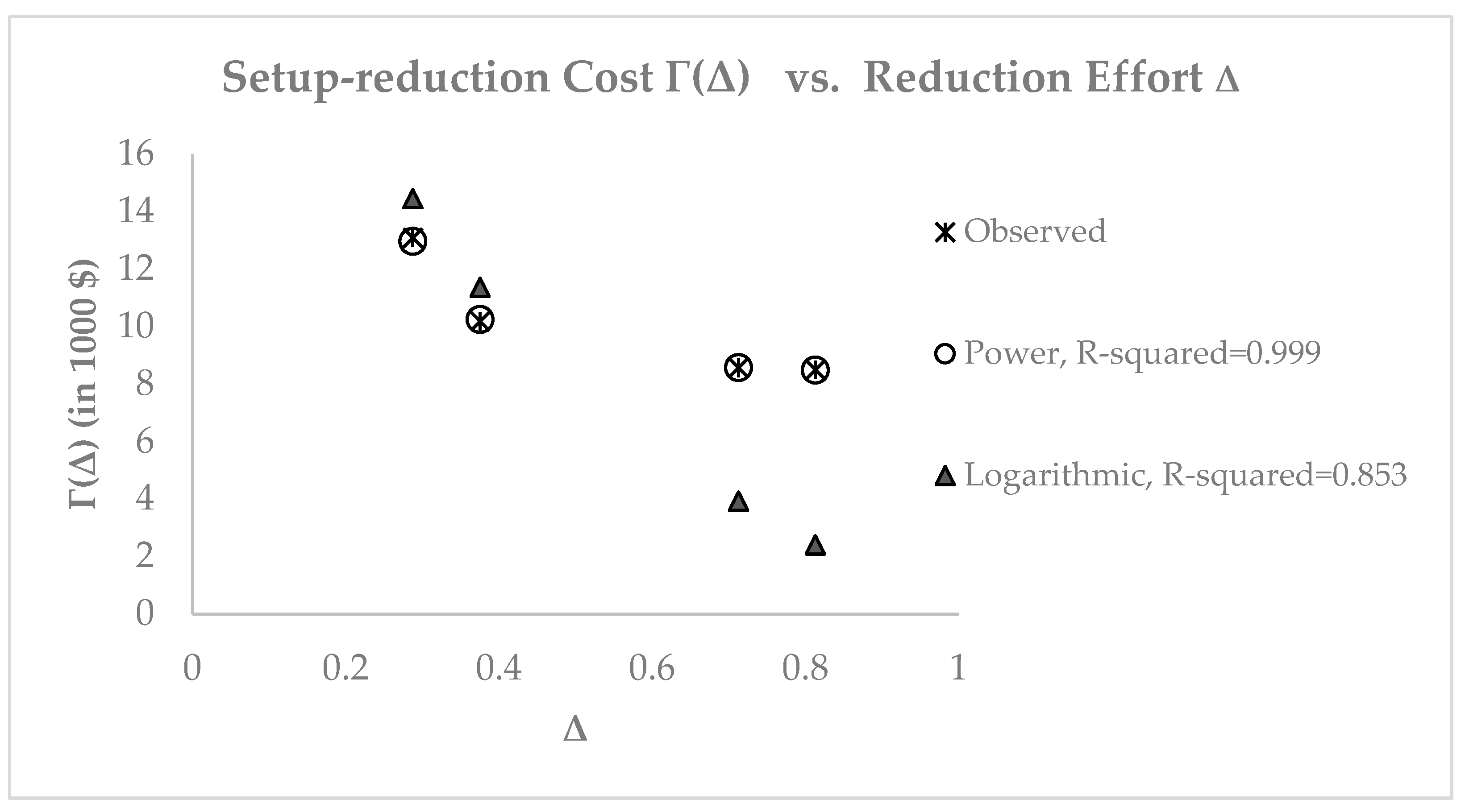has a corresponding R-squared = 0.853 (see Figure 1). Note that $\Gamma (\Delta =1)\equiv 0$ because no action would incur no cost. The logarithmic form has been suggested and widely studied in literature for analytical purposes. However, the power function form of reduction costs arises naturally from fundamental economic activities, as we elucidate later. Thus, there is a gap in the literature for a bottom-up approach to constructing setup-reduction cost functions aside from mere analytical convenience. We attempted to carry this out by using the so-called economic production functions.

Aside from a theoretical justification of a specific cost function, such an approach is also beneficial from an organizational resource perspective. Currently, there is no study in the literature that addresses the resource needs explicitly for setup-reduction efforts. This paper assumes that setup-reduction activity is an input conversion process: capital (equipment, tools, and automation) and labor are combined to achieve the desired reduction. For example, a manager may purchase a new press that allows for faster changeovers (reducing the setup time and related cost) by utilizing more capital or assigning more workers to a changeover operation to achieve the same result. A product design change that would result in faster changeover times might require the firm’s capital and labor investments. We take this bottom-up approach in this work to represent the setup-reduction efforts. Our approach to utilizing economic production functions to represent setup-reduction efforts justifies models in the literature that use convex power functions. We provide closed-form solutions for the resulting setup levels and the required inputs (resources) to be allocated to that purpose. As such, our findings bridge the decision areas of process improvement and resource planning.

There is a vast literature on the setup-reduction problem. Below, we review the literature focusing on the works that are most relevant in terms of demand stochasticity, accounting for shortages, and functional forms for setup-reduction costs.

In the presence of randomness in demands during lead times, the lot size-reorder point $(Q,r)$ control policy is employed for inventory management in systems that are continuously monitored. (Periodic review policies and corresponding models are outside the scope of our work and, hence, are omitted in this review). The setup-reduction problem for the lot size-reorder point model with stochastic demand during lead time was first addressed in [10]. In their model, explicit shortage costs are charged per unit short, and setup-reduction costs are described by logarithmic and power functions of capital investment. Although the formulation is for general demands, the analysis and optimality results are restricted to the special cases of uniform and exponential demand distributions. Ref. [11] analyzes the special cases of geometric and exponential demands during lead time when shortage costs are explicitly accounted for by charging them per stockout instance per unit time and per unit short. Setup reduction is achieved by employing a logarithmic investment function. Following these early works, research has evolved in two directions: random yields in replenished quantities (defective deliveries) starting with [12] and lead-time-reduction option in conjunction with setup reductions following the deterministic model proposed in [13]. Models developed in either direction directly reduce to the basic setting as special cases: when the yield is 100% (expressed with a Dirac Delta function) and/or the lead-time reduction option is not executed.

The case when delivered orders contain random defectives is studied in [12]. They account for shortage costs explicitly in the objective function, and the assumed setup-reduction cost function is assumed to be logarithmic. Closed-form optimality results are derived for exponential and uniform demand distributions. Ref. [14] revisits the problem with a service constraint. However, they reformulate the service-level constraint through an approximation proposed in [15] and work with the worst-case scenario (upper bound) instead of the exact constraint. Ref. [16] extends this work by considering normally distributed demands and joint reductions in setups and lead times. Shortage costs are accounted for explicitly in the objective function. The authors use both logarithmic and power investment functions for setup reductions. Our work differs from theirs in that we impose a hard service-level constraint. Along the lines of [8], ref. [17] approximates this model when setup reduction costs are logarithmic. Generally distributed random yields and normally distributed demands are analyzed in [18]. Shortage costs are explicitly accounted for in the objective function. Capital investment in setup reduction is assumed to be logarithmic in the reduction amount. Ref. [19] extends the model to allow for lead time, setup reductions, and lead-lead-time-dependent backorder rates. The investment function for setup reductions is logarithmic. Shortage costs are explicitly included in the optimization but are then re-formulated by considering an upper bound as suggested in [15]. The resulting approximate model holds for any demand distribution.

Ref. [20] considers defective deliveries with setup and lead-time reductions in conjunction with normally distributed demands. Shortages are explicitly costed in the optimization, and setup reductions incur logarithmic costs. Finally, refs. [21,22] consider random demand environments for the lot size-reorder point model when setup costs are step functions corresponding to discrete levels of reduction possibilities. All of these works take lead times to be independent of replenishment quantities. Ref. [23] examines the case for when (manufacturing) lead time depends on the lot size. Specifically, they assume that it is the sum of the setup time and the time to produce the lot, as proposed by [24]. They assume that a service-level constraint is binding and that setup reduction is achieved by shortening the setup time. Aside from convexity, no specific functional form is assumed for time reduction cost, but an inversely proportional structure is used in the illustrative numerical example. The direct interaction between lead times and setup times implies that reduction efforts in setup times also decrease lead times; this renders their analysis fundamentally different from and not applicable to settings with lot-size-independent (delivery) lead times. Thus, we see that the setup-reduction problem for random demand environments with delivery lead times has yet to be analyzed in an exact manner under a hard service-level constraint. We attempt to fill this gap in the literature, as well. Next, we focus on positioning our study in the big picture of sustainable SC management.

In the face of the pressing climate crisis, outbreaks, social instabilities, and changing demographics and needs, sustainability is at the front and center of the business world, which runs on supply chains (c.f., [25]). Hence, the sustainable supply chain management literature has expanded (e.g., [26]). Parallel to advances in intelligent technologies and data storing and processing capacities, supply chain analytics has emerged as an enabler for better decision making with sustainability imperatives (see [27]). We note here that the risks arising from natural disasters, labor strikes, outbreaks, and political conflicts, unlike those attributable to coordination problems, disrupt and break supply chains [28], and require integrated management systems [29] to cope with them (see Figure 2). A recent case, COVID-19, has wreaked havoc on many SCs and exposed their fragilities [30]. This has propelled researchers to integrate resiliency and technological advances into models taking on the challenging task of synchronizing production, location/allocation, distribution, transportation, and inventory management. For example, ref. [31] proposes a resilient healthcare SC network while minimizing the design and operating, environmental, and social costs. Several papers have highlighted the use of intelligent technologies in supply chain planning and execution under disruptions (e.g., [32,33,34,35]).

As regulations press firms to disclose their environmental, social, and governance (ESG) impacts [36], SCs need to be better coordinated, transparent, engaged with their customers, and resilient and intelligent in minimizing “waste”. According to [37], industrial waste, a sign of inefficiency, surfaces in various ways, such as overproduction, unnecessary processing, stocking and transportation, and the making of defective products. Waste in both capital (e.g., materials, energy, the use of technology, the cost of unproductive time, and landfills) and in labor (e.g., unnecessary human errors, lack of adequate level of automation, and the cost of time to train workers) causes not only additional SC costs but also hurts sustainability. In short, the ill-operated processes (how and where products are produced, or services rendered) add additional costs. Hence, “leaning” the logistics systems (see [38]), such as minimizing setup times for discrete manufacturing or maximizing transport capacity utilization for retailers or carriers becomes a critical goal.

The analysis herein has implications in two such directions, as well. From the perspective of response to disruptions, our study provides explicit conditions on when and how much investments are desirable in setup-reduction efforts in the face of demand regime changes in terms of overall demand rates and lead-time demand variability. To the best of our knowledge, such conditions have yet to be theoretically investigated for setup-reduction efforts in the literature and, hence, this study. Coupled with resource-allocation decisions, our findings provide valuable guidelines for managers for research and development (R&D) activities in times of supply and demand uncertainties. From a sustainability perspective, our models offer a framework to investigate the impact of setup reductions on sustainability.

As greenhouse gas emissions have become a pressing global issue, the inventory literature has seen the emergence of sustainable operations. (See [39] and its references for a recent comprehensive review of green operations.) A particularly relevant stream of research regarding sustainability is on the celebrated EOQ models where setup and/or stock-keeping operations result in carbon emissions. Among these works, we cite the following: Ref. [40] studies an EOQ model under a cap-and-trade mechanism and discusses managing the carbon footprints in inventory control. Ref. [41] investigates how to incorporate carbon emissions concerns into the operational decision-making models. Ref. [42] revisits the EOQ model with a cap on carbon emissions and analytically supports the observations in [41]. Similarly, [43] addresses the inventory-replenishment problem and carbon emission reduction investment with varying carbon regulation settings. In Section 4, we briefly discuss how our model can be used to incorporate carbon emissions.

The contributions of this work can be summarized as follows. This paper is the first in the literature to adopt a resource-based approach to investigate process improvement efforts. This provides a justification for specific functional forms used in the literature. In particular, we model setup reductions via (economic) production functions considering factor efficiencies. For the least-cost process improvement level, we offer optimal levels of labor and capital investments and the corresponding inventory system’s optimal control variables: optimal reordering and replenishment quantity. This enables managers to plan for and allocate labor and capital inputs for R&D activities while optimizing inventory decisions under demand and lead-time uncertainty. The specific formulation of the stochastic inventory problem under a hard service constraint fills a gap in the inventory literature with setup-reduction efforts. Our results apply to any situation with fixed-replenishment opportunities in manufacturing and retail settings. As another contribution, we reaffirm and extend the results in the seminal work [5] using a bottom-up, nested optimization approach. Figure 2 displays a pictorial of the problem at hand.

The layout of this paper is as follows: In Section 2, we construct the cost functions and relate them to the existing literature, present the mathematical model of the problem, and cast the generic optimization model. Section 3 provides all the related optimality results and structural insights. Section 4 describes some extensions on the generic models and provides additional insights into how process improvements may impact resource planning and allocation, guard against disruptions, and impact sustainability for SC operations. Then, in Section 5, we support our analytical results with a small numerical example and sensitivity analyses. Finally, Section 6 concludes with some remarks and future research venues.

2. The Generic Model Formulation

Any process improvement incurs fixed costs. In times of technological disruptions and to enhance their resiliencies, supply chains must invest in process-improvement costs. Inventory management is a fundamental supply chain function in which one of the goals is to benefit from economies of scale. To that end, we build on an inventory model to optimize process-improvement costs (Recall Figure 2). The details of this generic model follow. The list of key notations is given in Abbreviations. Any other less-used notation is explained when needed in the remainder of the paper.

Consider a product to be manufactured (or replenished by a retailer) whose demand is random with a mean rate $D$ (units per unit time, say, per year). We assume that all the uncertainties in demand and delivery can be represented through demand during lead time. Demand during the lead time has a normal distribution with mean demand during lead time denoted by ${\mu }_{DL}$ and the standard deviation of demand during lead time denoted by ${\sigma }_{DL}$. There is a fixed cost $S$ per setup (or order) associated with every order; units on hand inventory cost at a rate of $H$ per unit per unit time held in stock. All unmet demand is backordered at a rate of $\pi$ with a desired annual service level (fraction of immediately unmet demand per year) $\eta$. Each unit is acquired at the cost of $P$. The inventory system employs a lot size-reorder point $(Q,r)$ policy. Making the conventional assumption of at most one outstanding order at any time, the reorder point $r={\mu }_{DL}+z{\sigma }_{DL}$ with the safety stock factor $z$ selected such that the annual service-level target is achieved: $\eta =[(D/Q)\mathcal{L}(z){\sigma }_{DL}]/D$ where $\mathcal{L}[z]$ denotes the loss function of a standard normal variable.

Then, the expected total operating cost per unit time can be written as follows:

$$OC(Q,r)=SD/Q+H[Q/2+(r-{\mu }_{DL})]+\pi \eta D+PD$$

(1)

For the given system parameters, the decision variables are the values of the inventory control policy variables $Q$ and $r$.

Proposition 1.

The cost-minimizing replenishment policy is to manufacture (or order) $Q^{\ast }$ whenever the inventory level hits $r^{\ast }(={\mu }_{DL}+z^{\ast }{\sigma }_{DL})$ where $Q^{\ast }=\sqrt{SD/H(1/2-\eta /(1-\Phi (z^{\ast }))}$ and $z^{\ast }$ uniquely solves ${[\mathcal{L}(z^{\ast })]}^2=SD{\eta }^2/[H(1/2-\eta /(1-\Phi (z^{\ast }))/{\sigma }_{DL}^2]$. Then, the ensuing optimal cost per unit time $O{C}^{\ast }$is given by

$$\begin{array}{cc}\hfill O{C}^{\ast }& =OC(Q=Q^{\ast },z=z^{\ast })\hfill \\ & =\sqrt{SDH}\left(\sqrt{(1-\Phi (z^{\ast })-2\eta )}/\sqrt{2(1-\Phi (z^{\ast }))}+\sqrt{2(1-\Phi (z^{\ast }))}/\sqrt{(1-\Phi (z^{\ast })-2\eta )}\right)\hfill \\ & +H{z}^{\ast }{\sigma }_{DL}+(\pi \eta +P)D\hfill \\ & =\sqrt{2SDH}\sqrt{{(1-\Phi (z^{\ast })-\eta )}^2/(1-\Phi (z^{\ast }))(1-\Phi (z^{\ast })-2\eta )}+H{z}^{\ast }{\sigma }_{DL}+(\pi \eta +P)D\hfill \end{array}$$

(2)

Proof of Proposition 1:

The necessary first-order condition (FOC) for optimality on Q gives $\partial OC(Q)/\partial Q=\partial /\partial Q\{SD/Q+HQ/2\}+\partial /\partial Q\left\{Hz{\sigma }_{DL}\right\}=0$ where $\partial z/\partial Q$ is obtained by differentiating both sides of the desired annual service-level condition $\eta =[(D/Q)\mathcal{L}(z){\sigma }_{DL}]/D$. Also, $\partial \mathcal{L}(z)/\partial z=-(1-\Phi (z))$, $\partial z/\partial Q=-\eta /[(1-\Phi (z)){\sigma }_{DL}]$. Then, $\partial OC(Q)/\partial Q=-SD/Q^2+H/2-H{\sigma }_{DL}\eta /[(1-\Phi (z)){\sigma }_{DL}]$ $=-SD/Q^2+H/2-H\eta /(1-\Phi (z))$ $=0$. Solving for the optimal replenishment quantity for a given $z$ value, we obtain $Q*|z=\sqrt{SD/H(1/2-\eta /(1-\Phi (z)))}$. Note that the second-order condition (SOC) ${\partial }^{2}z/\partial Q^2=\left[-\eta \varphi (z){\sigma }_{DL}/{[(1-\Phi (z)){\sigma }_{DL}]}^2\right]\left[-\eta /[(1-\Phi (z)){\sigma }_{DL}]\right]>0$ guarantees that the optimal quantity obtained minimizes the expected total cost rate. Substituting the conditional optimal quantity expression into the desired annual service-level expression and squaring both sides, the corresponding optimal safety stock factor $z^{\ast }$ is found to solve ${[\mathcal{L}(z^{\ast })]}^2=SD{\eta }^2/H(1/2-\eta /(1-\Phi (z^{\ast })))/{\sigma }_{DL}^2$. Direct substitution gives the optimal cost rate. This completes the proof. □

We see that the optimal batching decision and the resulting expected cost rate depend on both the fixed cost $S$ and, indirectly, the uncertainties faced by the operations as captured by ${\sigma }_{DL}$. To alleviate the negative impact of uncertainty, a firm may engage in improvement efforts in two ways. (i) Externally by trying to reduce ${\sigma }_{DL}$ directly through improving variabilities in demand, lead times, etc. (ii) Internally by reducing the fixed cost $S$. Extra-firm improvements typically involve other stakeholders who may show organizational resistance to change. It may also not be physically possible to eliminate the sources of uncertainties in times of crisis, as were experienced globally during the recent COVID-19 pandemic, which disrupted all supply chains. Intra-firm improvements, on the other hand, require less managerial burden due to direct control over operations and provide faster results. Therefore, we consider the latter option and focus on fixed-replenishment (setup or order) cost-reduction efforts.

With process-improvement efforts, the fixed cost $S$ associated with each replenishment becomes a managerial decision variable. A firm can reduce fixed costs through process improvements by employing capital (in terms of automation, equipment, etc.) and labor. Such process improvements have been very well documented. We represent the effective setup level as $S\doteq S_0\Delta$, where $S_0$ denotes the current setup level prior to reduction efforts and $\Delta \le 1$ is a scalar representing the reduction effort. Let $\Gamma (\Delta )$ denote the cost of achieving a $(1-\Delta )\times 100\%$ fixed-replenishment cost reduction.

We depart from the existing literature on setup-reduction efforts in a fundamental way. Instead of envisioning the ‘acquisition’ of available reduction technologies from outside at a specific cost, we consider an intra-firm technology development capability. We assume that internal technology development can be modeled via economic production functions. That is, $\Delta$ is an output of capital $K$ and labor $L$ input levels devoted to the reduction activity in the firm: $\Delta =\theta (K,L)$. In economics parlance, such input conversion relationships have been called “production functions”. (See, for example, [44] for a basic introduction to economic production functions to describe input conversion processes.) Currently, the firm is assumed to possess some inherent human know-how $L_0$ and technical capital stock $K_0$ so that $\theta (K_0,L_0)=1$. In other words, the firm could have achieved its current process capabilities and desired to improve them with additional labor $L^{\prime }$ and capital $K^{\prime }$ investments for process R&D. Thus, $\Delta =\theta (K^{\prime }+K_0,L^{\prime }+L_0)$. Additional labor and capital are acquired at unit variable costs $c_K$ and $c_L$, respectively. We assume that acquisition costs of inputs are (annually) amortized values but suppress the explicit cost of capital notation. Noting that current assets $K_0$ and $K_0$ are variable but fixed costs, $\Gamma (\Delta )\doteq c_K{K}^{\prime }+c_L{L}^{\prime }$.

In the presence of fixed-replenishment cost-reduction efforts, a cost-minimizing decision maker’s optimization problem involves the determination of (i) the optimal values of the inventory control policy parameters, $Q^{\ast }$ and $r^{\ast }$ or, equivalently, $z^{\ast }$($=(r^{\ast }-{\mu }_{DL})/{\sigma }_{DL}$), (ii) the optimal setup-reduction rate, ${\Delta }^{\ast }$ and (iii) the optimal allocation of capital and labor inputs to achieve that reduction, $K^{\prime }*({\Delta }^{\ast })$ and $L^{\prime }*({\Delta }^{\ast })$. Thus, we have a nested optimization problem.

$${{\rm P}}^0:\underset{Q,r}{\min }\left\{\underset{\Delta }{\min }\left\{\underset{K^{\prime },L^{\prime }}{\min }{Z}_0\left\{\begin{array}{l}=S_{0}D\Delta /Q+H[Q/2+(r-{\mu }_{DL})]+\pi \eta D+PD+[c_K{K}^{\prime }+c_L{L}^{\prime }]\\ \left|\begin{array}{l}\Delta =\theta (K^{\prime }+K_0,L^{\prime }+L_0),z=(r-{\mu }_{DL})/{\sigma }_{DL},\\ \eta Q=\mathcal{L}(z){\sigma }_{DL}\end{array}\right.\end{array}\right\}\right\}\right\}.$$

(3)

This nested optimization problem can be posed equivalently in different ways. The research problem at hand emerged in the literature as selecting the optimal setup level with a corresponding cost of setup reduction (Porteus). For consistency with the literature and elucidation of the impact of economic inputs, we also recast the optimization in this equivalent canonical form and state it as ${{\rm P}}^1$.

$${{\rm P}}^1:\underset{\Delta }{\min }{Z}_1\left\{\begin{array}{l}=\sqrt{2S_{0}DH\eta (1+\eta \Phi (z^{\ast })/2\eta \Phi (z^{\ast })}\sqrt{\Delta }+{\Gamma }^{\ast }(\Delta )\\ +[H{z}^{\ast }{\sigma }_{DL}+(\pi \eta +P)D]\left|\Delta \le 1,{[\mathcal{L}(z^{\ast })]}^2(1-\Phi (z^{\ast }))=2\eta S_{0}D\Delta /H{\sigma }_{DL}^2\right.\end{array}\right\}.$$

(4)

where $\Delta$ is now the non-negative decision variable and ${\Gamma }^{\ast }(\Delta )$ denotes the least cost of reducing the fixed-replenishment cost. That is, ${\Gamma }^{\ast }(\Delta )$ is the solution to problem ${{\rm P}}^2$ as in Equation (5).

$${{\rm P}}^2:\underset{K^{\prime }, L^{\prime }}{\min }\Gamma (\Delta )\left\{\left.=c_K{K}^{\prime }+c_L{L}^{\prime }\right|\Delta =\theta (K^{\prime }+K_0,L^{\prime }+L_0)\right\},$$

(5)

The functional form of ${\Gamma }^{\ast }(\Delta )$ depends on the adopted specific functional form of $\theta (•)$ and the solution type ($\widehat{j}$) when the least cost is achieved: a corner solution. $(\widehat{j}=0; L^{\prime }*=K^{\prime }*=0)$, a boundary $(\widehat{j}=1; L^{\prime }*>0, K^{\prime }*=0, \mathrm{or} \widehat{j}=2; L^{\prime }*=0, K^{\prime }*>0)$ or an interior solution $(\widehat{j}=3; L^{\prime }*>0, K^{\prime }*>0)$. Aside from their mathematical interpretation, the solution types also correspond, respectively, to the following input-usage policies: the no-change policy, the labor-reliant single input policy, the capital-reliant single input policy, and the dual input policy. Such specific input-usage policies may be of interest or even dictated to managers due to organizational factors such as freezes on new labor recruits, new capital expenditures, or business environment conditions such as labor shortages or inability to access new capital in crises.

To facilitate our exposition, let ${\theta }_{\widehat{j}}(•)$ and ${\widehat{\Gamma }}_{\widehat{j}}(\Delta )$ denote, respectively, the particular structure of the setup-reduction rate function and the corresponding least cost when a particular solution type $\widehat{j}$ is imposed. By definition, $\Delta =1$ and ${\widehat{\Gamma }}_{\widehat{j}}(\Delta ):=0$ for $\widehat{j}=0$. Then, ${\Gamma }^{\ast }(\Delta )=\underset{\widehat{j}}{\min }{\widehat{\Gamma }}_{\widehat{j}}(\Delta )$. Thus, the best input usage policy obtains the minimal cost of setup reduction in achieving a non-zero setup cost reduction ${\widehat{j}}^{\ast }(\Delta )=\arg \min \{{\Gamma }_{{}_{\widehat{j}}}^{\ast }(\Delta ):\widehat{j}=1,2,3\}$. There may be multiple optima for ${\widehat{j}}^{\ast }(\Delta )$ for a given reduction rate, corresponding to intersection points of least-costs for different input usage policies. In such cases, we will interpret ${\widehat{j}}^{\ast }(\Delta )$ as the smallest of the set. For example, ${\widehat{j}}^{\ast }(\Delta )$ = 1 if labor-reliant and capital-reliant single-input policies give the same reduction costs for $\Delta$. We emphasize that the model herein enables one to determine the value (or cost) of imposed input-usage policies and may be used to study R&D budget or labor constraints.

Next, we delineate the functional form of the setup-reduction rate function $\theta (•)$. For some forms of $\theta (•)$, one can a priori determine the range of system parameters for which a particular solution type would be the least-cost solution for any given reduction $\Delta$. The notion is identical to determining the demand ranges for which a particular process alternative is best in process-selection decisions. We discuss some examples later. However, in general, delineating such regions analytically seems practically intractable. Instead, the base problem is best solved by treating each solution type as a separate problem and choosing the feasible solution as the global optimal. In general, the optimal solution is obtained by considering four possible candidates. But, for certain functional forms, we provide sufficient conditions for only one solution type to be optimal.

Economic production functions are mathematical constructs invented to describe the existing characteristics of an economic activity in a particular setting. The suitability of a specific functional form can only be tested empirically for individual firms. As such, no one functional form can be viewed as the most applicable to all firms across all industries. That is, managers are not at liberty to select a production function to describe their own process-improvement efforts. Data on past projects would indicate an organization’s input-conversion capabilities to generate process improvements. Therefore, optimal decisions must be investigated within different formulations of process-improvement efforts via economic production functions.

In our analysis, we first consider the Cobb–Douglas production function, the most commonly used functional form in the literature. As demonstrated below, it is amenable to obtaining closed expressions for optimality results. Moreover, it results in a piecewise power function. Thereby, it provides a resource-based bottom-up justification of the commonly assumed technology acquisition cost structure in the operations management literature. However, the piecewise nature introduces novelties in optimality results heretofore not investigated in the literature. Subsequently, we present and discuss the Constant Elasticity of Substitution (CES) and Leontief production functions and their modeling and optimization implications.

3. Optimality and Structural Results for Different Production Functions

In this section, we derive analytical results for the optimal cost-reduction values (and their corresponding optimal values of capital and labor levels for each reduction-rate function). We begin our analysis with the Cobb–Douglas function.

The Cobb–Douglas production function is given by

$${\theta }_1=\theta (K,L)=A{K}^{{\beta }_K}{L}^{{\beta }_L}=A{(K^{\prime }+K_0)}^{{\beta }_K}{(L^{\prime }+L_0)}^{{\beta }_L},$$

(6)

where $A$ is interpreted as the productivity or technological efficiency for the overall conversion process, and the parameters ${\beta }_K$$(<0)$ and ${\beta }_L$$(<0)$ determine the elasticities of capital and labor inputs, respectively. The surrogate parameter $\rho \doteq {\beta }_K+{\beta }_L$ denotes the elasticity of scale, which shows the extent of the effect of changing inputs on the output. In 1928, Cobb and Douglas were the first to introduce this input–output relation based on capital stock, labor force, and GNP for the US manufacturing industries from 1899–1922 [45]. Since then, it has been widely applied to energy generation [46,47], for several labor-intensive sectors in Japan [48], for applications in paper, steel, and oil industries [49], for regional agricultural production in Türkiye [50], for supply chain operations [51], for the energy sector [52] and radio frequency identification (RFID) productivity in retail SCs [53].

Proposition 2.

When the fixed-replenishment cost-reduction rate is of the Cobb–Douglas form, the minimal cost of setup reduction in achieving a non-zero$(1-\Delta )\times 100\%$ fixed-replenishment cost reduction is obtained by the best input-usage policy ${\widehat{j}}^{\ast }(\Delta )=\arg \min \{{\Gamma }_{{}_{\widehat{j}}}^{\ast }(\Delta ):\widehat{j}=1,2,3\}$ with the optimal capital input level ${\widehat{K}}_{}^{\ast }(\Delta |{\widehat{j}}^{\ast })=\widehat{K^{\prime }}(\Delta |{\widehat{j}}^{\ast })+K_0$, the optimal labor input level ${\widehat{L}}_{}^{\ast }(\Delta |{\widehat{j}}^{\ast })=\widehat{L^{\prime }}(\Delta |{\widehat{j}}^{\ast })+L_0$, the corresponding minimal cost of setup reduction ${\Gamma }^{\ast }(\Delta )={\min }_{\widehat{j}}\{{\widehat{\Gamma }}_{\widehat{j}}(\Delta ):\widehat{j}=1,2,3\}$ where each input usage policy $\widehat{j}$ has the following properties. 

(a) 

Under the labor-reliant (single input) policy ($\widehat{j}=1$), the (least-cost) additional capital input is $\widehat{K^{\prime }}(\Delta |\widehat{j})=0$, the additional labor input is $\widehat{L^{\prime }}(\Delta |\widehat{j})={(\Delta /A)}^{1/{\beta }_L}{K}_0{}^{-{\beta }_K/{\beta }_L}-L_0$ and the corresponding minimal cost of fixed cost reduction is ${\Gamma }_1^{\ast }(\Delta )={\Psi }_1{\Delta }^{1/{\beta }_L}-{\psi }_1$ where ${\Psi }_1=c_L{(\Delta /A)}^{1/{\beta }_L}{K}_0{}^{-{\beta }_K/{\beta }_L}$ and ${\psi }_1=c_L{L}_0$.

(b) 

Under the capital-reliant (single input) policy ($\widehat{j}=2$), the (least-cost) additional labor input is $\widehat{L^{\prime }}(\Delta |\widehat{j})=0$, the additional capital input is $\widehat{K^{\prime }}(\Delta |\widehat{j})={(\Delta /A)}^{1/{\beta }_K}{L}_0{}^{-{\beta }_L/{\beta }_K}-K_0$ and the corresponding minimal cost of fixed cost reduction ${\Gamma }_2^{\ast }(\Delta )={\Psi }_2{\Delta }^{1/{\beta }_K}-{\psi }_2$ where ${\Psi }_2=c_K{(\Delta /A)}^{1/{\beta }_K}{L}_0{}^{-{\beta }_L/{\beta }_K}$ and ${\psi }_1=c_K{K}_0$.

(c) 

Under the dual input policy ($\widehat{j}=3$), the least-cost additional labor input $\widehat{L^{\prime }}(\Delta |\widehat{j})$, the least-cost additional capital input $\widehat{K^{\prime }}(\Delta |\widehat{j})$ and the corresponding minimal cost of fixed cost reduction ${\Gamma }_3^{\ast }(\Delta )$ follow.

$$\begin{array}{c}{\widehat{K}}^{\prime }*(\Delta |\widehat{j}*)={({\Omega }^{-{\beta }_L}\Delta /A)}^{1/\rho }-K_0, \\ {\widehat{L}}^{\prime }*(\Delta |\widehat{j}*)={({\Omega }^{{\beta }_K}\Delta /A)}^{1/\rho }-L_0,\\ {\widehat{\Gamma }}_3^{}(\Delta )={\Psi }_3{\Delta }^{1/\rho }-{\psi }_3,\end{array}$$

(7)

where $\Omega =c_K{\beta }_L/c_L{\beta }_K={\widehat{L}}_{}^{\ast }(\Delta |\widehat{j}*)/{\widehat{K}}_{}^{\ast }(\Delta |\widehat{j}*)$, $\rho ={({\beta }_K+{\beta }_L)}^{}$, ${\Psi }_3=k_1{c}_K+k_2{c}_L$, $k_1={\left({\Omega }^{{\beta }_L}A\right)}^{-1/\rho }$, $k_2={\left({\Omega }^{-{\beta }_K}A\right)}^{-1/\rho }$, and the final term $\psi =c_K{K}_0+c_L{L}_0$.

Proof of Proposition 2.

Setting $\theta =\Delta$ in Equation (6) and solving for labor input, we obtain $L^{\prime }+L_0={\left(\Delta {(K^{\prime }+K_0)}^{-{\beta }_K}/A\right)}^{1/{\beta }_L}$ and accordingly from Equation (5), we can derive $\Gamma (\Delta )=c_K{K}^{\prime }+c_L{L}^{\prime }=c_K{K}^{\prime }+c_L{\left(\Delta {(K^{\prime }+K_0)}^{-{\beta }_K}/A\right)}^{1/{\beta }_L}-\left(c_K{K}_0+c_L{L}_0\right)$. For the boundary solutions, the least-cost value of the non-zero input can be obtained directly. For the boundary solution type $\widehat{j}=1$, suppressing the solution type notation for inputs, we obtain $L^{\prime }*+L_0={\left(\Delta K_0{}^{-{\beta }_K}/A\right)}^{1/{\beta }_L}$ and ${\Gamma }_{{}_{\widehat{j}}}^{\ast }(\Delta )=c_L{\left(\Delta K_0{}^{-{\beta }_K}/A\right)}^{1/{\beta }_L}-c_L{L}_0=\left[c_L{\left(K_0{}^{-{\beta }_K}/A\right)}^{1/{\beta }_L}\right]{\Delta }^{1/{\beta }_L}-c_L{L}_0$. For the boundary solution type $\widehat{j}=2$, we obtain $K^{\prime }*+K_0={\left(\Delta L_0{}^{-{\beta }_L}/A\right)}^{1/{\beta }_K}$ and ${\Gamma }_{{}_{\widehat{j}}}^{\ast }(\Delta )=\left[c_K{\left(L_0{}^{-{\beta }_L}/A\right)}^{1/{\beta }_K}\right]{\Delta }^{1/{\beta }_K}-c_K{K}_0$. For the interior solutions ($\widehat{j}=3$), via standard multivariable calculus, from FOCs, obtaining $K^{\prime }*$ such that $\partial {\Gamma }_3(\Delta )/\partial K^{\prime }*=0$ and rewriting $L^{\prime }$ in terms of $K^{\prime }*$, we derive the following optimal capital and labor levels. Once the expressions $K^{\prime }*$ and $L^{\prime }*$ are plugged into $\Gamma (\Delta )$, after some algebra, we find the closed-form optimality expressions as in Equation (7). □

Next, we determine the sufficiency conditions on the system parameters for the best input-usage policy given in Corollary 1 below.

Corollary 1.

When the setup cost-reduction rate is of the Cobb–Douglas form, the best input-usage policy giving the minimal cost of fixed-replenishment cost reduction in achieving a non-zero $(1-\Delta )\times 100\%$ fixed cost reduction follows.

(a) 

If $\Delta >\max \left\{A{\Omega }^{{\beta }_L}{K}_0{}^{\rho }, A{\Omega }^{-{\beta }_K}{L}_0{}^{\rho }\right\}$, the best input usage policy achieving the least cost for $\Delta$ is the dual input usage policy (${\widehat{j}}^{\ast }(\Delta )=3$) and ${\Gamma }^{\ast }(\Delta )={\widehat{\Gamma }}_3(\Delta )$.

(b) 

If $\Delta \le \max \left\{A{\Omega }^{{\beta }_L}{K}_0{}^{\rho }, A{\Omega }^{-{\beta }_K}{L}_0{}^{\rho }\right\}$, $c_L{(\Delta /A)}^{1/{\beta }_L}{K}_0{}^{-{\beta }_K/{\beta }_L}-c_L{L}_0\le c_K{(\Delta /A)}^{1/{\beta }_K}{L}_0{}^{-{\beta }_L/{\beta }_K}-c_K{K}_0$, then the best input-usage policy achieving the least cost for $\Delta$ is the labor-reliant single input-usage policy (${\widehat{j}}^{\ast }(\Delta )=1$) and ${\Gamma }^{\ast }(\Delta )={\widehat{\Gamma }}_1(\Delta )$.

(c) 

If $\Delta \le \max \left\{A{\Omega }^{{\beta }_L}{K}_0{}^{\rho }, A{\Omega }^{-{\beta }_K}{L}_0{}^{\rho }\right\}$, $c_L{(\Delta /A)}^{1/{\beta }_L}{K}_0{}^{-{\beta }_K/{\beta }_L}-c_L{L}_0>c_K{(\Delta /A)}^{1/{\beta }_K}{L}_0{}^{-{\beta }_L/{\beta }_K}-c_K{K}_0$ then, the best input-usage policy achieving the least cost for $\Delta$ is the capital-reliant single-input-usage policy (${\widehat{j}}^{\ast }(\Delta )=2$) and ${\Gamma }^{\ast }(\Delta )={\widehat{\Gamma }}_2(\Delta )$.

(d) 

If the initial capital and labor endowments $K_0$ and $L_0$ have been chosen according to the marginal cost condition $c_K\partial \Gamma (\Delta )/\partial L_0=c_L\partial \Gamma (\Delta )/\partial K_0$, then it is always optimal to use the dual-input policy.

Proof of Corollary 1.

The conditions (a)–(c) on the parameters follow immediately from solving for positive additional inputs. Condition (d) follows the same logic behind the relationship obtained between the additional inputs in the preceding Proposition 2, $c_K{\beta }_L/c_L{\beta }_K={\widehat{L}}_{}^{\ast }(\Delta |{\widehat{j}}^{\ast })/{\widehat{K}}_{}^{\ast }(\Delta |{\widehat{j}}^{\ast })$. This condition also holds for total inputs under the dual-input-usage policy. □

Note that when $\theta (•)$ is of the Cobb–Douglas form, the least cost of achieving $\Delta$ is a power function under each input usage policy. Hence, the technology acquisition costs of the power function form used in the literature have a theoretical foundation in economic production functions. But the overall least cost ${\Gamma }^{\ast }(\Delta )$, the minimum of all reduction costs arising from the three different input usage policies for any given $\Delta$, is a piecewise power function expressed via power functions that are valid only over specific intervals. Therefore, when technology is produced in-house, there is not a single power function that represents a reduction cost for all reduction rates. In this way, our work differs from the research in the extant literature.

Next, we consider the Constant Elasticity of Substitution (CES) production function of the form

$${\theta }_3=\theta (K,L)={\left({\alpha }_1{(K^{\prime }+K_0)}^{{\beta }_K}+{\alpha }_2{(L^{\prime }+L_0)}^{{\beta }_L}\right)}^{\gamma }$$

(8)

where $\gamma$ determines the elasticities of the inputs and of the overall transformation, and the other parameters are the same as in Equations (3) and (4). To ensure decreasing rates of return on capital and labor inputs, we assume $\gamma {\beta }_L<0$ and $\gamma {\beta }_K<0$. The CES production function was initially proposed in 1961 by Arrow et al. in a particular form where ${\beta }_K={\beta }_L=\beta$ and $\gamma =-{\beta }^{-1}$ [54]. Since then, it has been generalized to allow for different elasticities and has been successfully used in energy generation (e.g., [55]) and automation studies (e.g., [56]).

Proposition 3.

When the fixed-replenishment cost-reduction rate is of a special case CES form (${\beta }_K={\beta }_L=\beta$, $\gamma =-1/\beta$), the minimal cost of fixed-cost reduction in achieving a non-zero $(1-\Delta )\times 100\%$ fixed-cost reduction is obtained by the best input-usage policy ${\widehat{j}}^{*}(\Delta )=\arg \min \{{\Gamma }_{{}_{\widehat{j}}}^{\ast }(\Delta ):\widehat{j}=1,2,3\}$ with the optimal capital input level ${\widehat{K}}_{}^{\ast }(\Delta |\widehat{j}*)=\widehat{K^{\prime }}(\Delta |{\widehat{j}}^{\ast })+K_0$ , the optimal labor input level ${\widehat{L}}_{}^{\ast }(\Delta |{\widehat{j}}^{\ast })=\widehat{L^{\prime }}(\Delta |{\widehat{j}}^{\ast })+L_0$ , the corresponding minimal cost of setup reduction ${\Gamma }^{\ast }(\Delta )={\min }_{\widehat{j}}\{{\widehat{\Gamma }}_{\widehat{j}}(\Delta ):\widehat{j}=1,2,3\}$ where each input usage policy $\widehat{j}$has the following properties.

(a) 

Under the labor-reliant (single input) policy ($\widehat{j}=1$), the (least-cost) additional capital input is $\widehat{K^{\prime }}(\Delta |\widehat{j})=0$, the additional labor input is $\widehat{L^{\prime }}(\Delta |\widehat{j})={[(1/{\alpha }_L){\Delta }^{-\beta }-({\alpha }_K/{\alpha }_L)K_0{}^{\beta }]}^{1/\beta }-L_0$ and the corresponding minimal cost of setup reduction is ${\widehat{\Gamma }}_1^{}(\Delta )=c_L{[(1/{\alpha }_L){\Delta }^{-\beta }-({\alpha }_K/{\alpha }_L)K_0{}^{\beta }]}^{1/\beta }-c_L{L}_0$.

(b) 

Under the capital-reliant (single input) policy ($\widehat{j}=2$), the (least-cost) additional labor input is $\widehat{L^{\prime }}(\Delta |\widehat{j})=0$, the additional capital input is $\widehat{K^{\prime }}(\Delta |\widehat{j})={[(1/{\alpha }_K){\Delta }^{-\beta }-({\alpha }_L/{\alpha }_K)L_0{}^{\beta }]}^{1/\beta }-K_0$ and the corresponding minimal cost of setup reduction is ${\widehat{\Gamma }}_2^{}(\Delta )=c_K{[(1/{\alpha }_K){\Delta }^{-\beta }-({\alpha }_L/{\alpha }_K)L_0{}^{\beta }]}^{1/\beta }-c_K{K}_0$.

(c) 

Under the dual-input policy ($\widehat{j}=3$), the least-cost additional labor input $\widehat{L^{\prime }}(\Delta |\widehat{j})$, the least-cost additional capital input $\widehat{K^{\prime }}(\Delta |\widehat{j})$ and the corresponding minimal cost of fixed-cost reduction ${\widehat{\Gamma }}_3^{}(\Delta )$ follow:

$$\begin{array}{c}(\widehat{K^{\prime }}(\Delta |\widehat{j})+K_0)/(\widehat{L^{\prime }}(\Delta |\widehat{j})+L_0)={\left(c_L{\alpha }_K/c_K{\alpha }_L\right)}^{1/(\beta -1)}\\ \widehat{K^{\prime }}(\Delta |\widehat{j})={\Delta }^{-1}{\left[{\alpha }_K+{\alpha }_L{\left(c_L{\alpha }_K/c_K{\alpha }_L\right)}^{\beta /(\beta -1)}\right]}^{-1/\beta }-K_0, \\ \widehat{L^{\prime }}(\Delta |\widehat{j})={\Delta }^{-1}{\left[{\alpha }_L+{\alpha }_K{\left(c_K{\alpha }_L/c_L{\alpha }_K\right)}^{\beta /(\beta -1)}\right]}^{-1/\beta }-L_0,\\ {\Gamma }_3^{\ast }(\Delta )={\Psi }_3{\Delta }^{-1}-{\psi }_3,\end{array}$$

(9)

where ${\Psi }_3=c_K{\left[{\alpha }_K+{\alpha }_L{\left(c_L{\alpha }_K/c_K{\alpha }_L\right)}^{\beta /(\beta -1)}\right]}^{-1/\beta }$ and the final term ${\psi }_3=c_K{K}_0$. Equivalently, ${\Psi }_3=c_L{\left[{\alpha }_L+{\alpha }_K{\left(c_K{\alpha }_L/c_L{\alpha }_K\right)}^{\beta /(\beta -1)}\right]}^{-1/\beta }$ and the last term ${\psi }_3=c_L{L}_0$.

Proof of Proposition 3.

For the boundary solutions, the least-cost value of the non-zero input can be obtained directly. For the interior solutions ($\widehat{j}=3$), via standard multivariable calculus, we obtain $\partial K^{\prime }/\partial L^{\prime }=-({\alpha }_L/{\alpha }_K){(L/K)}^{\beta -1}$ and $\partial L^{\prime }/\partial K^{\prime }=-({\alpha }_K/{\alpha }_L){(K/L)}^{\beta -1}$. From FOC by applying the chain rule, we obtain $K^{\prime }*$, which is found to be inversely proportional to $\Delta$ and vice versa. Similar relationships hold for $K^{\prime }*$. Substitution into $\Gamma (\Delta )$ gives the closed-form optimality expressions as in Equation (9). □

For the CES production function, the least cost is inversely proportional to the fixed-cost reduction rate $\Delta$ when the best input usage policy employs both additional labor and capital for improvement efforts. The sufficiency conditions on the system parameters for this case are given below.

Corollary 2.

When the setup cost reduction rate is of the CES form, the best input-usage policy giving the minimal cost of setup reduction in achieving a non-zero $(1-\Delta )\times 100\%$ setup-cost reduction is the dual-input-usage policy (${\widehat{j}}^{\ast }(\Delta )=3$) and ${\Gamma }^{\ast }(\Delta )={\widehat{\Gamma }}_3(\Delta )$if

(a) 

$\Delta >max\left\{K_0{\left[{\alpha }_K+{\alpha }_L{\left(c_L{\alpha }_K/c_K{\alpha }_L\right)}^{\beta /(\beta -1)}\right]}^{1/\beta }, L_0{\left[{\alpha }_L+{\alpha }_K{\left(c_K{\alpha }_L/c_L{\alpha }_K\right)}^{\beta /(\beta -1)}\right]}^{1/\beta }\right\}$, or

(b) 

the initial capital and labor endowments $K_0$ and $L_0$ have been chosen according to the marginal cost condition $K_0/L_0={\left(c_L{\alpha }_K/c_K{\alpha }_L\right)}^{1/(\beta -1)}$.

Proof of Corollary 2.

The condition on the initial endowments $K_0$ and $L_0$ satisfies the marginal cost balance $c_K\partial \Delta /\partial L_0=c_L\partial \Delta /\partial K_0$ and, thereby, reasonably precludes suboptimal decision making prior to current process improvement efforts. □

Proposition 4.

When the reduction cost rate is of CES form, the optimal reduction rate ${\Delta }^{\ast }$, optimal replenishment quantity $Q^{\ast }$ and reorder point $r^{\ast }$ are given by the simultaneous solution of the following relationships:

$$\begin{gathered} {\left[({\alpha }_L/c_L)S_{0}D/Q^{\ast }\right]}^{\beta /(1-\beta )}{\Delta }^{\ast }{}^{2\beta }+{\Delta }^{\ast }{}^{\beta }{\alpha }_K{K}_0{}^{\beta }/{\alpha }_L-1/{\alpha }_L=0, \\ Q^{\ast }=\sqrt{2D{S}_0(1-\Phi (z^{\ast }))/H\eta }\sqrt{{\Delta }^{\ast }}, \end{gathered}$$

 and $r^{\ast }={\mu }_{DL}+z^{\ast }{\sigma }_{DL},$ where $z*$ solves ${[\mathcal{L}(z^{\ast })]}^2(1-\Phi (z^{\ast }))=2\eta S_{0}D{\Delta }^{\ast }/H{\sigma }_{DL}^2$.

Proof (sketch) of Proposition 4.

Rests on standard multivariate calculus and the necessary FOCs. □

Aside from this special case, CES is not amenable to obtaining closed-form expressions for optimal reduction efforts and requires numerical methods. For completeness, we provide the following result on the optimal decision variables.

Proposition 5.

Under the dual-input-usage policy, the optimal reduction rate, replenishment quantity and the reorder point for CES follow:

$${\Delta }^{\ast }={\left[S_{0}D{\Psi }_3{}^2/[H(1/2-\eta /((1-\Phi (z)){\sigma }_{DL}))]\right]}^{1/3},$$

$$Q^{\ast }={\left[S_{0}D{\Psi }_3/{[H(1/2-\eta /((1-\Phi (z)){\sigma }_{DL}))]}^2\right]}^{1/3},$$

 and $r^{\ast }={\mu }_{DL}+z^{\ast }{\sigma }_{DL}$ where $z^{\ast }$ solves $\eta Q^{*}=\mathcal{L}(z){\sigma }_{DL}$.

Proof of Proposition 5.

Having already obtained ${\widehat{\Gamma }}_{\widehat{j}}(\Delta )$, the nested optimization is carried out by first optimizing on $\Delta$ for given inventory-control policy parameters and then optimizing the policy parameters themselves. First, note that $TC(\Delta |Q,r)=S_{0}D\Delta /Q+HQ/2+H(r-{\mu }_{DL}){\sigma }_{DL}+PD+\pi \eta D+{\Psi }_3{\Delta }^{-1}-{\psi }_3$. From the SOC, ${\partial }^{2}TC/\partial {\Delta }^2=2{\Psi }_3{\Delta }^{-3}>0$, meaning $TC$ is strictly convex in $\Delta$. Therefore, the FOC gives the unique minimizer $\Delta *|Q,r=\sqrt{{\Psi }_{3}Q/S_{0}D}$. The expected total cost rate can now be written in terms of only the inventory-control policy parameters:

$$\begin{array}{cc}\hfill TC(Q,r)& =\sqrt{S_{0}D{\Psi }_3}{Q}^{-1+1/2}+HQ/2+H(r-{\mu }_{DL}){\sigma }_{DL}+PD+\pi \eta D+{\Psi }_3\sqrt{S_{0}D/{\Psi }_3}{Q}^{-1/2}-{\psi }_3\hfill \\ & =2\sqrt{S_{0}D{\Psi }_3}{Q}^{-1/2}+HQ/2+H(r-{\mu }_{DL}){\sigma }_{DL}+PD+\pi \eta D-{\psi }_3\hfill \end{array}$$

FOC on $Q$ given $z$ is $\partial TC/\partial Q=-\sqrt{S_{0}D{\Psi }_3}{Q}^{-3/2}+H(1/2-\eta {\sigma }_{DL}/((1-\Phi (z)){\sigma }_{DL}))=0$. Solving for $Q$, we obtain $Q^{\ast }={\left[S_{0}D{\Psi }_3/{[H(1/2-\eta /((1-\Phi (z)){\sigma }_{DL}))]}^2\right]}^{1/3}$ with $z^{\ast }$ satisfying the service-level condition. Noting that the SOC ${\partial }^{2}TC/\partial Q^{}=(3/2)\sqrt{S_{0}D{\Psi }_3}{Q}^{-5/2}-H\eta /({(1-\Phi (z))}^2)(-\eta /(1-\Phi (z)){\sigma }_{DL})>0$ guarantees optimality. Substitution of all entities gives the result

$$\begin{array}{cc}\hfill {\Delta }^{\ast }& =\sqrt{{\Psi }_3/S_{0}D}{\left[S_{0}D{\Psi }_3/{[H(1/2-\eta /((1-\Phi (z)){\sigma }_{DL}))]}^2\right]}^{1/6}\hfill \\ & ={(S_{0}D)}^{1/6-1/2}{\Psi }_3{}^{1/6+1/2}{\left[H(1/2-\eta /((1-\Phi (z)){\sigma }_{DL}))\right]}^{-1/3}\hfill \\ & ={\left[S_{0}D{\Psi }_3{}^2/[H(1/2-\eta /((1-\Phi (z)){\sigma }_{DL}))]\right]}^{1/3},\hfill \end{array}$$

$Q^{\ast }={\left[S_{0}D{\Psi }_3/{[H(1/2-\eta /((1-\Phi (z)){\sigma }_{DL}))]}^2\right]}^{1/3}$, and $r^{\ast }={\mu }_{DL}+z^{\ast }{\sigma }_{DL}$ where $z*$ solves $\eta {\left[S_{0}D{\Psi }_3/{[H(1/2-\eta /((1-\Phi (z)){\sigma }_{DL}))]}^2\right]}^{1/3}=\mathcal{L}(z){\sigma }_{DL}$. This completes the proof. □

Finally, we consider the Leontief production function which is of the form

$${\theta }_2=\theta (K,L)=\min \left(A_K{(K^{\prime }+K_0)}^{{\beta }_K},A_L{(L^{\prime }+L_0)}^{{\beta }_L}\right),$$

(10)

where $A_K$ and $A_L$ denote the productivity or technological efficiencies of the capital and labor inputs, respectively, and the parameters ${\beta }_K$$(<0)$ and ${\beta }_L$$(<0)$ are the corresponding input elasticities, as in Equation (3). Leontief introduced this functional form in 1947 [57]. The Leontief production function assumes that the inputs are complementary to each other. The Leontief production function may also represent the settings where, typically, changes in the production process and product characteristics are not possible in the short term. Among the applications, we refer to [46] for the steam power industry in the U.S.; [58] for various industries such as petroleum refining, primary metals, and electric power; [48] for sectors with large-quantity processing, large-scale assembly production, and capital-intensive technology; and [59] for the iron and steel industry in Japan.

Proposition 6.

When the reduction cost rate is of Leontief form, the best input-usage policy is always a dual-input policy, and the optimal capital input level ($K_{}^{\ast }(\Delta )={\widehat{K^{\prime }}}_3(\Delta )+K_0$), the optimal labor input level ($L_{}^{\ast }(\Delta )={\widehat{L^{\prime }}}_3(\Delta )+L_0$), the corresponding minimal cost of setup reduction ${\Gamma }_{}^{\ast }(\Delta )$ in achieving a $(1-\Delta )\times 100\%$ setup-cost reduction follow.

$$\begin{array}{c}{K}_{}^{\ast }(\Delta )={\left(\Delta /A_K\right)}^{1/{\beta }_K}, \\ L_{}^{\ast }(\Delta )={\left(\Delta /A_K\right)}^{1/{\beta }_L},\\ {\Gamma }_{}^{\ast }(\Delta )=c_K\left[{\left(\Delta /A_K\right)}^{1/{\beta }_K}-K_0\right]+c_L\left[{\left(\Delta /A_L\right)}^{1/{\beta }_L}-L_0\right].\end{array}$$

(11)

Proof (sketch) of Proposition 6.

Similar to the proof of Proposition 1, but this time with the setup-cost-reduction rate being in the form of Leontief production function, i.e., ${\theta }_2$ in Equation (10). □

Thus, when improvement efforts are represented via the Leontief production function, the firm must devote additional labor and capital to achieve fixed-cost reductions. The resulting least cost is a polynomial in $\Delta$ and does not lend itself to closed-form expressions for the optimal fixed-cost reduction rate. However, the optimality results for $P^1$ can be established from first-order conditions as stated below.

Corollary 3.

When the reduction cost rate is of Leontief form, the optimal reduction rate ${\Delta }^{\ast }$, optimal replenishment quantity $Q^{\ast }$ and reorder point $r^{\ast }$ are given by the simultaneous solution of the following relationships:

$$S_{0}D/Q+(c_K/{\beta }_K){\Delta }^{*}{}^{(1-{\beta }_K)/{\beta }_K}{\left(1/A_K\right)}^{1/{\beta }_K}+(c_L/{\beta }_L){\Delta }^{*}{}^{(1-{\beta }_L)/{\beta }_L}{\left(1/A_L\right)}^{1/{\beta }_L}=0,$$

$Q^{\ast }=\sqrt{2D{S}_0(1-\Phi (z^{\ast }))/H\eta }\sqrt{{\Delta }^{\ast }}$, and $r^{\ast }={\mu }_{DL}+z^{\ast }{\sigma }_{DL}$, where $z*$ solves ${[\mathcal{L}(z^{\ast })]}^2(1-\Phi (z^{\ast }))=2\eta S_{0}D{\Delta }^{\ast }/H{\sigma }_{DL}^2$.

For both the Leontief and general CES functional forms, one can also recommend very versatile conic quadratic solution techniques in practice (e.g., [60,61]).

Having derived the optimality results for the input levels and the total setup cost reduction cost, we are now ready to determine the conditions for and find the optimal level of reduction effort, ${\Delta }^{\ast }$. We encapsulate these results in Proposition 7.

When setup-reduction efforts are expressed by Cobb–Douglas in general and equal input elasticity CES functions under the dual-input-usage policy (c.f., Propositions 1 and 3), the optimal setup-reduction cost, ${\Gamma }^{\ast }(\Delta )$, is a power function of the form $\kappa {\Delta }^{-\lambda }-\phi$, where $\Delta \in [0,1]$, $\lambda >0$, and $\phi >0$; this is the cost structure assumed in [5] and the majority of the following research stream. Thus, we can establish that the power function form of the setup-reduction cost directly follows from the fundamental economic production functions and may be verified in empirical settings. Conversely, an approach utilizing economic production functions to represent setup-reduction efforts justifies models in the literature that use convex power functions. The optimal setup-reduction level can be obtained directly from the result in [5], which we recast in Proposition 7.

Proposition 7.

Suppose that ${\Gamma }^{\ast }(\Delta )=\kappa {\Delta }^{-\lambda }-\phi$ with $\Delta \in [0,1]$, $\lambda >0$, and $\phi >0$. Then, the optimal reduction rate ${\Delta }^{\ast }$, replenishment quantity $Q^{\ast }$, and reorder point $r^{\ast }$follow.

$${\Delta }^{\ast }={\left[\lambda \kappa /S_{0}D\right]}^{1/(1+\lambda )}{Q}^{\ast }{}^{1/(1+\lambda )},$$

$$Q^{\ast }={\left[\lambda \left[S_{0}D{\left[\lambda \kappa /S_{0}D\right]}^{1/(1+\lambda )}+\kappa {\left[\lambda \kappa /S_{0}D\right]}^{-\lambda /(1+\lambda )}\right]/\left[(1+\lambda )H(1/2-\eta /(1-\Phi (z^{\ast })))\right]\right]}^{(1+\lambda )/(1+2\lambda )},$$

and $r^{\ast }={\mu }_{DL}+z^{\ast }{\sigma }_{DL}$, where $z^{\ast }$ solves $\eta Q^{\ast }=\mathcal{L}(z^{\ast }){\sigma }_{DL}$.

Proof of Proposition 7.

Recall $TC(\Delta ,Q,z)=S_0\Delta D/Q+H(Q/2+z{\sigma }_{DL})+\pi \eta D+PD+{\Gamma }^{\ast }(\Delta )$. The FOC on $\Delta$ gives ${\Delta }^{\ast }|Q,z={\left[\lambda \kappa /S_{0}D\right]}^{1/(1+\lambda )}{Q}^{1/(1+\lambda )}$. Substituting the conditional best reduction rate, the expected total cost rate can be cast as $TC(\Delta ,Q,z)=S_{0}D{\left(\frac{\lambda \kappa }{S_{0}D}\right)}^{\frac{1}{1+\lambda }}{Q}^{1/(1+\lambda )-1}+H\left(\frac{Q}{2}+z{\sigma }_{DL}\right)+\pi \eta D+PD+\kappa {\left(\frac{\lambda \kappa }{S_{0}D}\right)}^{\frac{-\lambda }{1+\lambda }}{Q}^{-\lambda /(1+\lambda )}-\phi$. Then, by collecting the terms, we obtain $TC(\Delta ,Q,z)=\left[S_{0}D{\left(\frac{\lambda \kappa }{S_{0}D}\right)}^{\frac{1}{1+\lambda }}+\kappa {\left(\frac{\lambda \kappa }{S_{0}D}\right)}^{\frac{-\lambda }{1+\lambda }}\right]Q^{-\lambda /(1+\lambda )}+H\left(\frac{Q}{2}+z{\sigma }_{DL}\right)+\pi \eta D+PD-\phi$. The FOC on $Q$ gives $\partial TC(Q,z)/\partial Q=0$ resulting in

$$\left[S_{0}D{\left[\lambda \kappa /S_{0}D\right]}^{1/(1+\lambda )}+\kappa {\left[\lambda \kappa /S_{0}D\right]}^{-\lambda /(1+\lambda )}\right](-\lambda /(1+\lambda ))Q^{-\lambda /(1+\lambda )-1}+H(1/2+{\sigma }_{DL}\partial z/\partial Q)=0$$

Solving for $Q$ gives $Q^{\ast }|z$ as follows: $Q^{\ast }|z={\left[\lambda \left[S_{0}D{\left[\lambda \kappa /S_{0}D\right]}^{1/(1+\lambda )}+\kappa {\left[\lambda \kappa /S_{0}D\right]}^{-\lambda /(1+\lambda )}\right]/\left[(1+\lambda )H(1/2+{\sigma }_{DL}\partial z/\partial Q)\right]\right]}^{(1+\lambda )/(1+2\lambda )}$, and rearranging terms and expanding over the term with the derivative, we obtain $Q^{\ast }|z={\left[\lambda \left[S_{0}D{\left[\lambda \kappa /S_{0}D\right]}^{1/(1+\lambda )}+\kappa {\left[\lambda \kappa /S_{0}D\right]}^{-\lambda /(1+\lambda )}\right]/\left[(1+\lambda )H(1/2-\eta /(1-\Phi (z)))\right]\right]}^{(1+\lambda )/(1+2\lambda )}$, where, at optimality, $z^{\ast }$ satisfies $Q^{\ast }\eta =\mathbb{L}(z^{\ast }){\sigma }_{DL}$. Noting that ${\partial }^{2}TC(Q,z)/\partial Q^2=\tilde{A}(-\lambda /(1+\lambda ))(-(1+2\lambda )/(1+\lambda ))Q^{-(1+2\lambda )/(1+\lambda )-1}+H{\sigma }_{DL}{\partial }^{2}z/\partial Q^2>0$, where $\tilde{A}=\left[S_{0}D{\left[\lambda \kappa /S_{0}D\right]}^{1/(1+\lambda )}+\kappa {\left[\lambda \kappa /S_{0}D\right]}^{-\lambda /(1+\lambda )}\right]>0$, we show the convexity and the joint optimality. □

Finally, we consider a special case of Proposition 7 in which the parameters are now considered rather deterministic, and the lead times are insignificant (i.e., assumed to be 0). When there are no uncertainties in the system (regarding demand and supply deliveries) and negligible lead times, the inventory setting reduces to that studied in [5]. Demand is now constant with the rate $D$ (units per unit time), and delivery lead time is negligible. In our notation, we set ${\mu }_{DL}$, ${\sigma }_{DL}$ and $\eta$ to zero; we retain the rest of the setting and notation. In this setting, the optimal continuous control policy is known to be of the EOQ- type, in which the total cost per unit time for an order size $Q$ is $TC(Q)=QS/D+QH/2+PD$. Then, $Q*=\arg \min \{TC(Q):Q>0\}=\sqrt{2DS/H}$, i.e., the EOQ. Thus, the cost-minimizing ordering policy is to manufacture (or order) $Q*$ whenever the inventory level hits zero. Then, the ensuing optimal cost per unit time is given by $TC(Q=Q*)=\sqrt{2DSH}+PD.$ The setup-reduction optimization problem now becomes ${{\rm P}}^{\mathrm{D}}:\underset{\Delta }{\min }Z\left\{\left.=\sqrt{2DH{S}_0\Delta }+PD+{\Gamma }^{\ast }(\Delta )\right|\Delta \ge 0\right\}$, where $\Delta$ and ${\Gamma }^{\ast }(\Delta )$ are as defined before.

Corollary 4.

Suppose ${\Gamma }_{\widehat{j}}^{\ast }(\Delta )={\Psi }_{\widehat{j}}{\Delta }^{a_{\widehat{j}}}-{\psi }_{\widehat{j}}$. Then, the optimal setup-reduction rate is given by ${\Delta }^{*}=-(1/2{\Psi }_{\widehat{j}}{a}_{\widehat{j}}){[2S_{0}DH]}^{1/(2a_{\widehat{j}}-1)}$. If this much reduction were to be implemented under the input-usage policy $j$, then the resulting setup-reduction cost would be ${\widehat{\Gamma }}_j({\Delta }_{\widehat{j}}^{*})={\Psi }_j{(-(1/2{\Psi }_{\widehat{j}}{a}_{\widehat{j}}){[2S_{0}DH]}^{1/(2a_{\widehat{j}}-1)})}^{a_j}-{\psi }_j$.

4. Some Insights on Process Improvements for Sustainable Supply Chains

This section illustrates how the models herein may benefit managerial practice. We develop some extensions on our generic models and discuss the impact of resource planning and allocation, disruptions, and carbon emissions penalties.

4.1. Resource Planning and Allocation

Our construction of the setup-reduction costs employing multi-factor production functions enables managers to determine not only the optimal level of setup reduction but also the required labor and capital resources to achieve that. The resources are found to be one-to-one related to the reduction level, albeit nonlinearly. This is the most significant practical contribution of our models.

Furthermore, most changes in processes face resistance and incur fixed costs. Our models consider in-house process-improvement efforts, which reduce the likelihood of “change resistance” because the incumbent labor and management undertake a collective goal. An excellent example of such effective process improvements is the concept of a “quality circle,” in which a designated group of employees work toward a solution to a specific, smaller-scope problem in the company. While emerging intelligent technologies such as Blockchain and IoT seem promising in enhancing sustainability performance (a process improvement), caution needs to be taken when assessing the fixed cost of establishing their infrastructure and implementation. At that stage, our models may also be employed as tools for cost–benefit analysis. Consider, for instance, a dyadic supply chain with a retailer and a manufacturer. The retailer may optimize its scheduled deliveries from the manufacturer while the manufacturer synchronizes its production lots to be loaded on the retailer’s fleet of trucks. In such a case, a logistics service improvement could entail better coordinating the order–production–delivery process, which may be achieved by investing in an advanced transport management system. Then, both the manufacturer and the retailer can assess their current capital and labor constraints and decide on whether it will be more economical for them to invest in reducing their common fixed costs compared to the cost of purchasing and implementing alternative new technologies (c.f., [62]). Proposition 7 could be utilized in such a trade-off scenario.

4.2. Impact of Disruptions

We first consider the disruptive changes that may occur in the demand regimes. Disruptions may cause drastic changes in the average demand rate $D$, increases in demand variability, average delivery lead time, and lead-time variability. In some disruptions, as experienced during the recent pandemic, firms may desire or be obliged to satisfy a larger portion of the demand. Our models enable one to investigate the impact of these changes on setup-reduction efforts. We focus on the setup-reduction problem when reductions can be expressed through the Cobb–Douglas and equal input elasticity case of CES functions. As shown above, the setup-reduction cost function is of power form ${\Gamma }^{\ast }(\Delta )=\kappa {\Delta }^{-\lambda }-\phi$ in such instances. (All results are obtained from Proposition 7 using standard calculus; therefore, their derivations are omitted).

The impact of the average demand rate on the reorder point is given by $\partial r^{\ast }/\partial D={\sigma }_{DL}\partial z^{\ast }/\partial D$ where $\partial z^{\ast }/\partial D=-\eta /[{\sigma }_{DL}(1-\Phi (z^{\ast }))]\partial Q^{\ast }/\partial D$($<0$), which implies that the reorder point is decreasing in the average demand rate (due to the binding shortage constraint.) The impact of the lead-time demand variability is given by $\partial r^{\ast }/\partial {\sigma }_{DL}=z^{\ast }+{\sigma }_{DL}\partial z^{\ast }/\partial D$, where

$$\partial z^{\ast }/\partial {\sigma }_{DL}=\mathcal{L}(z^{\ast })/[{\sigma }_{DL}(1-\Phi (z^{\ast }))]-\eta /[{\sigma }_{DL}(1-\Phi (z^{\ast }))]\partial Q^{\ast }/\partial {\sigma }_{DL}.$$

The latter is nonnegative for nonnegative $z^{\ast }$ and positive otherwise, because the optimal lot size increases in the lead-time demand variability as shown below.

The impact of demand on the lot size is given by

$$\partial Q^{\ast }/\partial D=\frac{\lambda /[(1+\lambda )D]}{(1+2\lambda )/[(1+\lambda )Q^{\ast }]+{\eta }^2\varphi (z^{\ast })/[(1/2-\eta /(1-\Phi (z^{\ast }))){\sigma }_{DL}{(1-\Phi (z^{\ast }))}^3]}$$

and the impact of the lead-time demand variability on the lot size is given by

$$\partial Q^{\ast }/\partial {\sigma }_{DL}=\frac{\eta \varphi (z^{\ast })/[(1/2-\eta /(1-\Phi (z^{\ast }))){\sigma }_{DL}{(1-\Phi (z^{\ast }))}^3]}{(1+2\lambda )/[(1+\lambda )Q^{\ast }]+{\eta }^2\varphi (z^{\ast })/[(1/2-\eta /(1-\Phi (z^{\ast }))){\sigma }_{DL}{(1-\Phi (z^{\ast }))}^3]}.$$

We see that $0<\partial Q^{\ast }/\partial {\sigma }_{DL}<1/\eta$ and $0<\partial Q^{\ast }/\partial D<Q^{\ast }/D$.

The impact of the demand parameters on the optimal setup-reduction decision is attained by the comparative statics conditions $\partial {\Delta }^{\ast }/\partial D=[(1/Q^{\ast })\partial Q^{\ast }/\partial D-1/D]{\Delta }^{\ast }/(1+\lambda )$ and $\partial {\Delta }^{\ast }/\partial {\sigma }_{DL}=\left[{\Delta }^{\ast }/[(1+\lambda )Q^{\ast }]\right]\partial Q^{\ast }/\partial {\sigma }_{DL}$. Combining the two results, we obtain

$$\frac{\partial {\Delta }^{\ast }/\partial D}{\partial {\Delta }^{\ast }/\partial {\sigma }_{DL}}=\frac{\partial Q^{\ast }/\partial D}{\partial Q^{\ast }/\partial {\sigma }_{DL}}-\frac{Q^{\ast }}{D},$$

where

$$\begin{array}{l}\frac{\partial Q^{\ast }/\partial D}{\partial Q^{\ast }/\partial {\sigma }_{DL}}=\frac{\lambda /[(1+\lambda )D]}{\eta \varphi (z^{\ast })/[(1/2-\eta /(1-\Phi (z^{\ast }))){\sigma }_{DL}{(1-\Phi (z^{\ast }))}^3]}\\ =\frac{\lambda (1/2-\eta /(1-\Phi (z^{\ast }))){\sigma }_{DL}{(1-\Phi (z^{\ast }))}^3}{(1+\lambda )D\eta \varphi (z^{\ast })}.\end{array}$$

Hence,

$$\frac{\partial {\Delta }^{\ast }/\partial D}{\partial {\Delta }^{\ast }/\partial {\sigma }_{DL}}=\frac{\lambda (1/2-\eta /(1-\Phi (z^{\ast }))){\sigma }_{DL}{(1-\Phi (z^{\ast }))}^3}{(1+\lambda )D\eta \varphi (z^{\ast })}-\frac{Q^{\ast }}{D}.$$

We notice that $\partial {\Delta }^{\ast }/\partial D<0$ since $\partial Q^{\ast }/\partial D<Q^{\ast }/D$ and that $\partial {\Delta }^{\ast }/\partial {\sigma }_{DL}>0$. That is, as the average demand rate increases (decreases), the optimal setup reduction increases (decreases); however, as variability in the lead-time demand increases (decreases), the optimal setup reduction decreases (increases). Suppose the demand parameters in case of disruptions can be expressed through an underlying ‘disruption severity’ parameter, $u(\ge 0)$ as follows. Let $D=D_0+{\nu }_{D}u$ describe the average demand rate in the presence of a disruption with a base demand rate (prior to disruption) $D_0$ and a disruption sensitivity of ${\nu }_D$. Similarly, let ${\sigma }_{DL}={\sigma }_0+{\nu }_{\sigma }u$ account for the standard deviation of demand during lead time in the presence of a disruption with a base variability (prior to disruption) ${\sigma }_0$ and a disruption sensitivity of ${\nu }_{\sigma }$. Then, the overall impact of disruption on the optimal setup-reduction effort is cast as $\partial {\Delta }^{\ast }/\partial u=\frac{\partial {\Delta }^{\ast }}{\partial D}\frac{\partial D}{\partial u}+\frac{\partial {\Delta }^{\ast }}{\partial {\sigma }_{DL}}\frac{\partial {\sigma }_{DL}}{\partial u}$. Dividing that derivative by the positive term $\frac{\partial {\Delta }^{\ast }}{\partial {\sigma }_{DL}}$, we note that $\partial {\Delta }^{\ast }/\partial u<(>)0$ if $\left(\frac{\partial {\Delta }^{\ast }/\partial D}{\partial {\Delta }^{\ast }/\partial {\sigma }_{DL}}\right)\frac{\partial D}{\partial u}<(>)\frac{-\partial {\sigma }_{DL}}{\partial u}$.

We see that $\partial {\Delta }^{\ast }/\partial u<(>)0$ if $\frac{\partial {\Delta }^{\ast }}{\partial D}\frac{\partial D}{\partial u}<(>)\frac{-\partial {\Delta }^{\ast }}{\partial {\sigma }_{DL}}\frac{\partial {\sigma }_{DL}}{\partial u}$. Equivalently, if $\left(\frac{-\partial {\Delta }^{\ast }/\partial D}{\partial {\Delta }^{\ast }/\partial {\sigma }_{DL}}\right)\frac{\partial D}{\partial u}<(>)\frac{\partial {\sigma }_{DL}}{\partial u}$, then $\partial {\Delta }^{\ast }/\partial u<(>)0$. Now, let

$$U:=\frac{\partial {\Delta }^{\ast }/\partial D}{\partial {\Delta }^{\ast }/\partial {\sigma }_{DL}}=\frac{\partial Q^{\ast }/\partial D}{\partial Q^{\ast }/\partial {\sigma }_{DL}}-\frac{Q^{\ast }}{D}=\frac{\lambda (1/2-\eta /(1-\Phi (z^{\ast }))){\sigma }_{DL}{(1-\Phi (z^{\ast }))}^3}{(1+\lambda )D\eta \varphi (z^{\ast })}-\frac{Q^{\ast }}{D}.$$

By considering the conditions on $\partial {\Delta }^{\ast }/\partial u<(>)0$, we observe that some disruption scenarios necessitate (encourage) setup reductions, whereas, in others, keeping the current setup level is optimal. Specifically, we find the following.

It is optimal to keep the current setup level when (i) a disruption reduces the average demand rate (${\nu }_D<0$) and increases lead-time demand variability (${\nu }_{\sigma }>0$). This case was observed for a wide range of consumer products as lockdowns decreased the demands and logistical bottlenecks increased delivery lead times.

It is optimal to engage in setup reduction only when a disruption (i) increases average demand rate (${\nu }_D>0$) and decreases lead-time demand variability (${\nu }_{\sigma }<0$), or (ii) increases both average demand rate and lead-time demand variability (${\nu }_D,{\nu }_{\sigma }>0$) and ${\nu }_{\sigma }/{\nu }_D<-U$, or (iii) decreases both average demand rate and lead-time demand variability (${\nu }_D,{\nu }_{\sigma }<0$ and ${\nu }_{\sigma }>-U{\nu }_D$. The first case occurred during the pandemic for medical equipment demands by healthcare facilities (such as face masks, staff gowns, etc.) for providers with government contracts; the second case occurred for companies that had to acquire them from unreliable suppliers. The last case refers to a setting where firms could only serve local markets with local suppliers.

We also see that $\partial {\Delta }^{\ast }/\partial \eta >0$; that is, optimal setup reduction increases as the desired service level decreases. This was also the case during the pandemic when businesses aimed to capture as much of the (reduced) demand as possible and to satisfy almost all of the demand for particular medical goods.

4.3. Incorporation of Carbon Emissions Penalties

Our model is versatile enough to provide a framework for analyzing the setup-reduction efforts and sustainability concerns. Specifically, it can be used for inventory settings where carbon emissions may be costly. We briefly sketch below how our model can be extended in that direction.

We retain all prior notations. In addition, we define unit carbon emissions as follows. Let ${\epsilon }_S,{\epsilon }_H,{\epsilon }_P,{\epsilon }_{\pi }$ denote the carbon emissions per setup, per unit of inventory held in stock per unit time, per unit of item acquired, and per unit short, respectively. Also, let ${\epsilon }_K,{\epsilon }_L$ denote the unit carbon emissions per unit of capital and labor employed per unit time. These would correspond to the carbon footprints of equipment and personnel. Suppose a carbon tax (or penalty) $\tau$ is charged per unit of carbon emissions.

We assume that when firms are engaged in setup-reduction activities, their efforts may result in an actual reduction of setup costs (as discussed above) and carbon emissions reductions. Specifically, we assume that setup cost is reduced to $S_0\Delta$ and carbon emissions due to a setup become $\zeta {\epsilon }_S\Delta$. Then, carbon emissions per unit time associated with operations are given by $e{m}_{OPS}=\zeta {\epsilon }_S\Delta D/Q+{\epsilon }_H[Q/2+(r-{\mu }_{DL})]+{\epsilon }_{P}D+\tau {\epsilon }_{\pi }\eta D$. Carbon emissions per unit time associated with capital and labor employed for setup-reduction efforts are given by $e{m}_{\Delta }={\epsilon }_K{K}^{\prime }+{\epsilon }_L{L}^{\prime }$. In the presence of carbon emissions from individual operations, the expected cost rate $T{C}^{CARBON}(Q,r,\Delta )$ consists of the operational costs of inventory management, setup-reduction costs, and carbon emissions taxes (or penalties.) Thus,

$$\begin{array}{c}T{C}^{CARBON}(Q,r,\Delta )=OC(Q,r)+{\Gamma }^{*}(\Delta )+\tau [e{m}_{OPS}+e{m}_{\Delta }]\\ =(S_0+\tau \zeta {\epsilon }_S)\Delta D/Q+(H+\tau {\epsilon }_H)[Q/2+(r-{\mu }_{DL})]+\pi \eta D+(P+\tau {\epsilon }_P)D\\ +[(c_K+\tau {\epsilon }_K)K^{\prime }+(c_L+\tau {\epsilon }_L)L^{\prime }]\end{array}$$

The new optimization problem in the presence of carbon emissions is written as

$${{\rm P}}^{CARBON}:\underset{Q,r}{\min }\left\{\underset{\Delta }{\min }\left\{\underset{K^{\prime },L^{\prime }}{\min }{Z}_0\left\{\begin{array}{l}=\{S_0+\tau \zeta {\epsilon }_S\}\Delta D/Q+\{H+\tau {\epsilon }_H\}[Q/2+(r-{\mu }_{DL})]+\{\pi +\tau {\epsilon }_{\pi }\}\eta D+\{P+\tau {\epsilon }_P\}D+[\{c_K+\tau {\epsilon }_K\}{K}^{\prime }+\{c_L+\tau {\epsilon }_L\}{L}^{\prime }]\\ \left|\begin{array}{l}\Delta =\theta (K^{\prime }+K_0,L^{\prime }+L_0),z=(r-{\mu }_{DL})/{\sigma }_{DL},\\ \eta Q=L(z){\sigma }_{DL}\end{array}\right.\end{array}\right\}\right\}\right\}.$$

(12)

The modified optimization problem in Equation (12) is identical in all properties if one redefines the cost parameters in curly brackets. Thus, all of our conclusions above also hold for this case.

5. Numerical Examples

In this section, we illustrate by way of numerical examples the impact of disruptions on setup-reduction efforts. The base case has the following system parameters. The setup-reduction cost is of power form with $K=\$\mathrm{32,500}$, $\lambda =0.25$, and $\phi =\$\mathrm{32,500}$. This assumes a one-time investment of $250,000 annualized at a rate of 15%. The base average demand rate per unit time, $D_0=\mathrm{100,000}$ with base lead-time demand standard deviation ${\sigma }_{DL}^0=D_0/3$. The unit holding cost rate is $H=\$10$ and the setup cost before improvements is $S_0=\$1000$ per setup. The average demand rate is taken as 1.0, 0.9, and 0.8 multiples of $D_0$, corresponding to disruption scenarios of 10% and 20% decreases. The variability of the lead-time demand is taken as 0.05, 0.1, 0.2, and 0.4 multiples of the base variability, corresponding to decreasing and increasing variabilities during disruptive demand regime changes. Three different service levels are considered: $\eta =1\%, 2\%$ and $5\%$. The optimal lot size, safety stock factor, and setup reduction are presented in

Table 1. Optimal lot size $Q^{\ast }$, optimal safety stock factor $z^{\ast }$ and optimal setup reduction ${\Delta }^{\ast }$ in response to disruptive demand regime changes ($\lambda =0.25$, $K=\mathrm{32,500}$, $\phi =\mathrm{32,500}$, $D_0=\mathrm{100,000}$, $D=D_0$, ${\sigma }_{DL}^0=D_0/3$, $H=10$, $S_0=1000$).

$\mathit{\eta }$	${\mathit{\sigma }}_{\mathit{D}\mathit{L}}/{\mathit{\sigma }}_{\mathit{D}\mathit{L}}^0$	${\mathit{Q}}^{\ast }$	${\mathit{z}}^{\ast }$	${\Delta }^{\ast }$
0.01	0.05	7628.2	1.29	0.68
	0.1	8748.3	1.54	0.76
	0.2	11,041.7	1.74	0.92
	0.4	11,128.7	1.98	1.00
0.02	0.05	7825.4	0.93	0.70
	0.1	9082.2	1.	0.78
	0.2	11,522.0	1.42	0.95
	0.4	11,978.4	1.68	1.00
0.05	0.05	8257.9	0.35	0.73
	0.1	9702.5	0.68	0.83
	0.2	8927.7	1.11	1.00
	0.4	14,073.2	1.22	1.00

,

Table 2. Optimal lot size $Q^{\ast }$, optimal safety stock factor $z^{\ast }$ and optimal setup reduction ${\Delta }^{\ast }$ in response to disruptive demand regime changes ($\lambda =0.25$, $K=\mathrm{32,500}$, $\phi =\mathrm{32,500}$, $D_0=\mathrm{100,000}$, $D=0.9D_0$, ${\sigma }_{DL}^0=D_0/3$, $H=10$, $S_0=1000$).

$\mathit{\eta }$	${\mathit{\sigma }}_{\mathit{D}\mathit{L}}/{\mathit{\sigma }}_{\mathit{D}\mathit{L}}^0$	${\mathit{Q}}^{\ast }$	${\mathit{z}}^{\ast }$	${\Delta }^{\ast }$
0.01	0.05	7523.9	1.30	0.73
	0.1	8664.1	1.55	0.82
	0.2	10,849.5	1.74	0.98
	0.4	11,280.1	1.99	1.00
0.02	0.05	7717.2	0.94	0.75
	0.1	8924.1	1.21	0.84
	0.2	7760.2	1.58	1.00
	0.4	12,189.2	1.69	1.00
0.05	0.05	8141.0	0.36	0.78
	0.1	9603.1	0.69	0.89
	0.2	8683.5	1.12	1.00
	0.4	13,351.0	1.22	1.00

and

Table 3. Optimal lot size $Q^{\ast }$, optimal safety stock factor $z^{\ast }$ and optimal setup reduction ${\Delta }^{\ast }$ in response to disruptive demand regime changes ($\lambda =0.25$, $K=\mathrm{32,500}$, $\phi =\mathrm{32,500}$, $D_0=\mathrm{100,000}$, $D=0.8D_0$, ${\sigma }_{DL}^0=D_0/3$, $H=10$, $S_0=1000$).

$\mathit{\eta }$	${\mathit{\sigma }}_{\mathit{D}\mathit{L}}/{\mathit{\sigma }}_{\mathit{D}\mathit{L}}^0$	${\mathit{Q}}^{\ast }$	${\mathit{z}}^{\ast }$	${\Delta }^{\ast }$
0.01	0.05	7406.4	1.31	0.80
	0.1	8495.6	1.55	0.89
	0.2	7260.3	1.90	1.00
	0.4	10,635.0	1.99	1.00
0.02	0.05	7595.5	0.95	0.81
	0.1	8819.6	1.22	0.92
	0.2	7697.1	1.60	1.00
	0.4	11,492.1	1.69	1.00
0.05	0.05	8009.8	0.37	0.85
	0.1	9487.1	0.70	0.97
	0.2	8409.7	1.13	1.00
	0.4	13,680.3	1.23	1.00

.

The behavior of the decision variables confirms the theoretical sensitivity analysis: as the demand rate decreases (increases), the optimal setup reduction $(1-{\Delta }^{*})\%$ decreases (increases), whereas lead-time demand variability has the opposite effect. Tightening (loosening) the service level also increases (decreases) the optimal setup reduction.

6. Concluding Remarks and Future Research

In this paper, we incorporated the capital and labor levels as endogenous decision variables in optimizing in-house process-improvement efforts embedded in the classical $(Q,r)$ inventory system widely used when the demand and lead time are probabilistic—mostly the case in practice. In so doing, we utilized production functions that relate two inputs (capital and labor) to the output efficiency (production level). To the best of our knowledge, this is the first study to consider a resource-based approach to construct such cost functions in process improvements.

We identified the conditions under which closed-form solutions exist. Notably, for each of the production functions considered (Cobb–Douglas, CES, and Leontief), we provided the conditions under which optimal interior or boundary solutions exist, ascertaining uniqueness. These structural analytical results were obtained via multivariate calculus (first- and second-order conditions), and we showed joint convexity.

In particular, we built on and extended the setup cost reduction model developed in [5]. Exposed in the forms of propositions and corollaries, our structural results provide neat, closed-form solutions for optimal input levels (capital and labor) and inventory control variables (reorder point and replenishment quantity) to achieve the optimal cost of (in-house) process improvement level (i.e., setup cost reduction effort) for a given inventory service (i.e., safety stock) level, all while the uncertainties in both demand and the delivery/manufacturing lead time are accounted for. In the end, via Proposition 7, we bring together all the production functions considered (Cobb–Douglas, CES, and Leontief) and unify them in the form of a general power function—a crucial step toward implementable analytical results in developing decision tools for lean inventory systems in supply chain management. Our analysis of published data (see Figure 1) supports the importance and illustrates possible verification of the multi-input functions we considered in this paper.

Albeit stylized, our models enable tractable solutions and general, robust insights. Sensitivity analysis on the optimal decision variables reveals that (1) as the demand rate decreases (increases), the optimal setup reduction $(1-{\Delta }^{\ast })\%$ decreases (increases); (2) lead-time demand variability has the opposite effect; and (3) tightening (loosening) the service level also increases (decreases) the optimal setup reduction. This is verified in an illustrative numerical study.

Lastly, we generalized the model to incorporate taxes/penalties for carbon emissions. This framework can be utilized to investigate the sustainability impacts of process improvements in future work.

We hope our prescriptive models and new structural results in this paper will germinate numerous research ideas. It would be interesting, for example, to analyze industry-specific data and see how each production function best fits for which type of SC (e.g., responsive vs. efficient). In the context of sustainable SCs, an imminent study may explore process improvement and design problems through the lenses of economic, environmental, social, and cultural imperatives. It is worthwhile to develop a formal model that optimizes process leanness and resiliency of SCs under disruptions. Some other future research could investigate the optimal timing of process improvement efforts for competing SCs, and how external risks due to the ramifications of climate change (a significant disruption) can be integrated into SC decision support systems.