Article

Altitude Correction of GCM-Simulated Precipitation Isotopes in a Valley Topography of the Chinese Loess Plateau

1
Key Laboratory of Resource Environment and Sustainable Development of Oasis of Gansu Province, College of Geography and Environmental Science, Northwest Normal University, Lanzhou 730070, China
2
Atmosphere and Ocean Research Institute, University of Tokyo, Tokyo 169-8555, Japan
3
Laboratory of Atmospheric Physics, Department of Physics, University of Patras, GR-26500 Patras, Greece
4
Laboratoire de Météorologie Dynamique, IPSL, CNRS, Sorbonne Université, 75006 Paris, France
*
Author to whom correspondence should be addressed.
Sustainability 2023, 15(17), 13126; https://doi.org/10.3390/su151713126
Submission received: 27 July 2023 / Revised: 23 August 2023 / Accepted: 30 August 2023 / Published: 31 August 2023

Abstract

:
Altitude is one of the important factors influencing the spatial distribution of precipitation, especially in a complex topography, and simulations of isotope-enabled climate models can be improved by altitude correlation. Here we compiled isotope observations at 12 sites in Lanzhou, and examined the relationship between isotope error and altitude in this valley in the Chinese Loess Plateau using isoGSM2 isotope simulations. Before altitude correction, the performance using the nearest four grid boxes to the target site is better than that using the nearest box; the root mean square error in δ18O using the nearest four grid boxes averagely decreases by 0.37‰ compared to that using the nearest grid boxes, and correlation coefficient increases by 0.05. The influences of altitude on precipitation isotope errors were examined, and the linear relationship between altitude error and isotope simulations was calculated. The strongest altitude isotopic gradient between δ18O mean bias error and altitude error is in summer, and the weakest is in winter. The regression relationships were used to correct the simulated isotope composition. After altitude correction, the root mean square error decreases by 1.21‰ or 0.86‰ using the nearest one or four grid boxes, respectively, and the correlation coefficient increases by 0.13 or 0.08, respectively. The differences between methods using the nearest one or four grids are also weakened, and the differences are 0.02‰ for root mean square error and −0.01 for the correlation coefficient. The altitude correction of precipitation isotopes should be considered to downscale the simulations of climate models, especially in complex topography.

1. Introduction

As natural tracers of hydrological circulation, the stable hydrogen and oxygen isotopes in precipitation are sensitive to modern and historical environmental changes [1,2,3]. Isotope fractionations occur when water vapor evaporates, condenses, transports, and mixes, which results in complex spatial patterns and temporal variations of precipitation isotopes [4,5,6]. The global samplings of precipitation isotopes dated back to the mid-20th century, and a number of observations since then provide a useful tool to understand the isotope tracers in the water cycle [7,8,9]. The environmental signals in modern precipitation isotopes on an annual or even longer timescale are also an important basis to reconstruct climate in the past using proxies [10,11,12]. The existing isotope datasets longer than 30 years are still very limited, and the spatial distribution of sampling sites is uneven, which makes it difficult to examine the long-term hydrological and climate controls on precipitation isotopes [13,14].
Isotope-enabled climate models, especially the general circulation models (GCM), are useful to acquire the continuous time series of precipitation isotopes at various time scales [15,16,17]. Due to atmospheric dynamics in the climate models, the isotope-enabled simulation is considered to be an important supplementary to in situ measurements. However, the spatial resolutions of climate models are usually coarse, and many topography-related information is smoothened. The performances of prediction models vary greatly in large spatial scale, with usually good performance in plain areas and poor simulation in complex terrains [18,19], indicating the importance of altitude correction of precipitation isotopes especially in a complex topography with large altitude fluctuation [20,21]. Compared to some global or regional long-term mean products of precipitation isotopes [22,23,24], the climate-model-derived simulation should be improved in spatial resolution, especially in small-scale cases with complex terrain, where altitude correction or downscaling is crucial for climate-model-simulated isotope data.
Usually, the precipitation isotopes negatively correlate with altitude in the mountains, which is also known as the altitude effect [25,26,27]. When the moisture transports along the upwind slope, the vapor condensation is usually associated with temperature and humidity at different altitudes and then causes a decreasing trend in isotope ratios as the altitude rises [28,29,30]. This provides a practical method to downscale or calibrate the climate-model-simulated isotopes. If the relationship between isotope or isotope error and altitude is identified, the knowledge of spatial patterns of precipitation isotopes in mountainous areas can be greatly improved. It should be noted that an isotope observation network with a small spatial domain and complex altitude is needed to establish this quantitative relationship, i.e., multiple sites with large altitude gradients are required to correct the precipitation isotopes using altitude.
Lanzhou is a valley city located at the upper Yellow River in western China, and there have been a number of precipitation isotope studies in past decades. Stable hydrogen and oxygen isotope compositions were analyzed at more than ten sites across this city, which provide a platform to examine the spatial representativity of precipitation isotopes in complex topography. In this study, we used two methods to correct simulated data of the isotope-incorporated global spectral model version 2 (isoGSM2) in Lanzhou, and examined the role of altitude on precipitation isotope simulations. The work aims to provide methods to improve the performance of isotope simulations in a complex topography in a specific location.

2. Materials and Methods
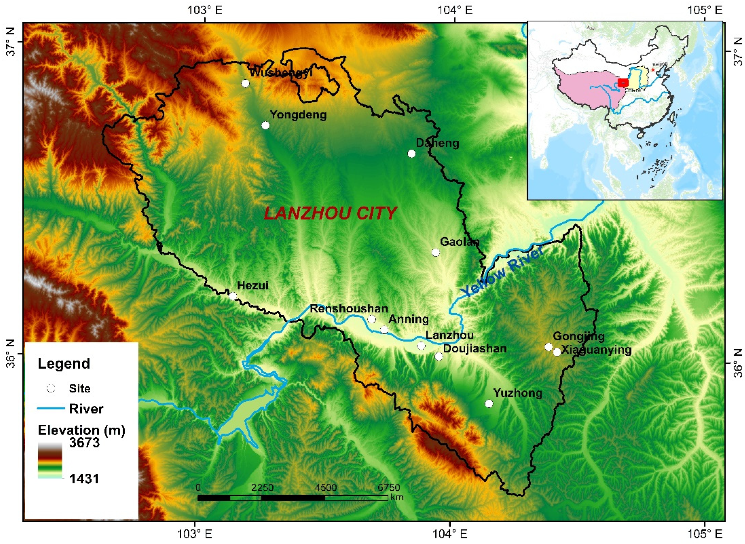
2.1. Study Area

Lanzhou (35°34′ N–37°00′ N, 102°36′ E–104°35′ E) is the capital city of Gansu Province in western China, and the area is approximately 13,100 km2 (Figure 1). As a valley city at the upper reaches of the Yellow River, the study area is located in the western part of the Chinese Loess Plateau, and is close to the eastern margin of the Qinghai–Tibet Plateau. The downtown area is distributed along a narrow valley, and the Yellow River goes across from west to east. The altitude of most areas ranges between 1500 and 3000 m a.s.l., and the downtown area is approximately 1500 m a.s.l. Located at the northwestern margin of the summer monsoon, the study area is jointly influenced by the monsoon and westerly moisture sources. Precipitation is mainly concentrated in the summer months.

2.2. Isotope Data

2.2.1. Measured Isotope Data

Here we compiled the stable water isotopes in precipitation observed across the study region in past decades (Table 1). There are 12 sampling sites acquired from three data sources: (1) the city-scale measurements during 2011–2014 [31]. From April 2011 to October 2014, there were four continuous sampling sites (Anning, Yuzhong, Gaolan, and Yongdeng); from October 2013 to October 2014, six additional sites were added (Renshoushan, Doujiashan, Wushengyi, Daheng, Gongjing, and Hezui). Here, the 1432 event-based precipitation samples collected from 2011–2014 were weighted to 196 monthly data using precipitation amounts. (2) The measurements in the Global Network of Isotopes in Precipitation (GNIP) Lanzhou site [32]. There are 39 monthly data of stable water isotopes from 1985–1987 and 1996–1999. (3) Measurements at Xiaguanying from April 2016 to October 2017 [33]. The event-based precipitation samples collected at Xiaguanying are weighted to 16 monthly data. Among the 12 sites, the altitude ranges between 1517 m (Lanzhou) and 2482 m (Gongjing).

2.2.2. Simulated Isotope Data

The precipitation isotopes at a 6 h interval (0:00, 6:00, 12:00, and 18:00 UTC) as well as corresponding surface air pressure from 1979 to 2020 were simulated using isoGSM2 [34]. This stable isotope-enabled general circulation model simulates high-resolution variations in stable isotopes in precipitation and water vapor, which has been applied to examine atmospheric water transport [35,36,37].
The stable oxygen isotope compositions are expressed as a delta notation relative to Vienna Standard Mean Ocean Water (VSMOW) as:
δ O   18 = q H 2   O   18 / q H 2 O R × 1000
where q is the content for water molecule of H218O or H2O, and R is the isotope ratio of 18O/16O.
The precipitation isotope data were weighted to a daily, monthly, or seasonal series using precipitation amount when necessary:
δ w = P i δ i P i
where δw is the weighted average isotope value, Pi is the precipitation amount, and δi is the original isotope value in precipitation. Seasons are defined as spring (March to May), summer (June to August), autumn (September to November), and winter (December to February).

2.3. Methods

2.3.1. Altitude-Correlation Method

Two methods are used to acquire the simulated precipitation isotopes at the target sites. For method 1, the isotope error and altitude error for each site are calculated using the simulated isotope value minus the observed isotope value. The simulated isotope values and altitude of the target site are replaced by those at the nearest grid box of the isoGSM simulations. The simulated altitude is based on the simulated surface air pressure using the barometric formula. The linear regression using the least square method is then conducted between the altitude error and isotope value error for spring, summer, autumn, and winter. The slope of the linear regression is used to correct the simulated isotope, when the altitude difference between the simulated and observed locations is known.
For method 2, to acquire the simulated isotope values and altitude for each site, the four nearest grid boxes are applied, which is different from method 1 in which only the nearest box is involved. The bilinear interpolation is conducted to synthesize the simulated isotope values and altitude at four locations into one target location. Then the linear regression is also used to correct the simulated isotope values using the altitude difference, which is similar to method 1.

2.3.2. Statistical Measures

Several statistical measures were used to evaluate the simulation, including root mean square error (RMSE), mean absolute error (MAE), mean bias error (MBE), and correlation coefficient (R).
The formula for RMSE is as follows:
R M S E = 1 n i = 1 n ( y i k i ) 2
where yi is the observed value, ki is the simulated value, and n is the number of samples. The smaller the RMSE, the closer the simulations are to the actual values.
The formula for MAE is as follows:
M A E = 1 n i = 1 n y i k i
where yi is the observed value, ki is the simulated value, and n is the number of samples. The smaller the MAE, the better the simulations are.
The formula for MBE is as follows:
M B E = i = 1 n ( k i y i ) n
where yi is the observed value, ki is the simulated value, and n is the number of samples. The smaller the MBE, the closer the simulations are to the observations.
The formula for calculating R is as follows:
R = i = 1 n ( y i y ¯ ) ( k i k ¯ ) i = 1 n ( y i y ¯ ) 2 i = 1 n ( k i k ¯ ) 2
where yi is the observed value, y ¯ is the average observed value, ki is the simulated value, k ¯ is the average of the simulated values, and n is the number of samples.

3. Results

3.1. Impact of Nearest One or Four Grid Boxes

Figure 2 shows the relationship between the simulated and observed monthly averages of δ18O in precipitation without altitude correction, and two methods using the nearest one (method 1) or four (method 2) grid boxes are applied for simulations. In general, the two methods have similar temporal trends in the study region. Among these sampling sites, the observed δ18O values in precipitation are usually higher than the simulations, that is, the simulations of isoGSM2 have more depleted isotopes than the observations in the study region.
Several statistical measures are used to examine the performance of methods using the near one or four grid boxes without altitude correction (Table 2). According to the arithmetic averages and medians of the statistical measures among these sampling sites, before altitude correction, the performance using the nearest four grid boxes (method 2) to the target site is better than that using the nearest box (method 1). The arithmetic averages of δ18O RMSE of methods 1 and 2 are 4.39‰ and 4.01‰, respectively, and the average difference in δ18O RMSE is 0.37‰. The median of the δ18O RMSE difference for each site is 0.22‰. Similarly, the averages of correlation coefficient are 0.52 and 0.57, respectively, indicating an increase by 0.05 from method 1 to method 2. The median of correlation coefficient difference for each site is also 0.05. The pattern for MAE and MBE also have similar findings.
For the GNIP Lanzhou site with the longest observations (Table 2), there is clear difference between methods 1 and 2. The δ18O RMSE values of methods 1 and 2 are 5.16‰ and 4.23‰, respectively. The latter is less than the former by 0.93‰, which is larger than the station average previously mentioned (0.37‰). The correlation coefficient of the methods 1 and 2 are 0.47 and 0.60, respectively, and there is an increase of 0.13 from method 1 to method 2.
It should be noticed that in the valley topography of the study area, the population is usually distributed at relatively lower altitudes close to the river, and then the sampling sites with manual supports usually have a lower altitude than the regional mean. This may cause a systemic bias that the low altitude may have larger weightings in observations, and the higher altitudes are not well represented by the existing observations. Specifically, the sites on the mountains or plateaus outside the urban area with low altitudes across the study region are limited. According to the altitude effect of precipitation isotopes, the high altitudes usually have a lower isotope value, and the sampling-caused bias may cause the simulated δ18O to be lower than the observations to some degree.

3.2. Relationship between Altitude Error and Simulation Performance

Figure 3 shows the relationship between altitude error and precipitation isotope simulation performance using the two methods. The negative correlation between altitude error and seasonal δ18O MBE can be seen for each season. As the altitude error increases, the isotope MBE decreases. The linear regression slopes of methods 1 and 2 are −0.20‰/100 m and −0.41‰/100 m in spring, −4.40‰/100 m and −4.22‰/100 m in summer, −1.27‰/100 m and −0.44‰/100 m in autumn, and −1.11‰/100 m and −1.49‰/100 m in winter, respectively. The strongest altitude isotopic gradient is in summer, and the weakest is in winter. Most seasons have a negative correlation coefficient ≤ −0.5, except winter with limited precipitation observations. For method 1, among the five sites with relatively long observations (Lanzhou, Anning, Yuzhong, Gaolan, and Yongdeng), the Yongdeng site has the smallest altitude error (25.5 m), while Lanzhou and Anning have the largest altitude errors (993.9 m and 962.9 m), respectively. For method 2, among the five sites with long observations, the Yongdeng site has the smallest elevation error of 62.1 m, while Lanzhou and Anning have the largest elevation errors (571.9 m and 585.8 m), respectively. Generally, the sites with low altitude errors correspond to the sites with better performance of precipitation isotopes according to the models. Between the two methods, the altitude error of method 1 is usually larger than that of method 2.

3.3. Improvement in Simulations Corrected by Altitude

Based on the relationship between seasonal δ18O MBE and altitude error, altitude correction can be conducted on the isoGSM2 monthly data. Assuming that the precipitation isotope fractionation and altitude gradient is a constant, the simulated results are corrected. Figure 4 shows the simulations after altitude correction as well as the observed values for each sampling site. Compared to Figure 2 and Table 2 before altitude correction, the accuracy of the simulated δ18O in precipitation shown in Figure 4 and Table 3 has been improved. In addition, the differences between methods using methods 1 and 2 are also weakened, and the average differences are 0.02‰ for root mean square error and −0.01 for correlation coefficient.
In Table 3, the arithmetic averages of RMSE among these sampling sites are 3.18‰ using method 1 and 3.16‰ using method 2, which are less than those before altitude correction (4.39‰ using method 1 and 4.01‰ using method 2). The arithmetic averages of correlation coefficient are 0.64 using method 1 and 0.66 using method 2, and are also higher than those before altitude correction (0.52 and 0.57). In the GNIP Lanzhou site, the RMSE values are 3.72‰ using method 1 and 3.56‰ using method 2, and are also better than those without correction (5.16‰ and 4.23‰).
The greater the altitude error, the more obvious the correction effect. The terrain of Lanzhou is complex, and the altitude of the simulated data does not match the actual altitude, resulting in differences in results. The two methods have different processes for obtaining altitude, and the error range of method 2 is relatively narrow. Through altitude correction, the model can more accurately simulate the variability in precipitation isotopes, thereby improving the consistency of evaluation indicators.
The Taylor diagram (Figure 5) [38] is used to compare the the two methods before and after correction. In Figure 5, scattered points represent interpolation methods, radial lines represent correlation coefficients, horizontal and vertical axes represent standard deviations, and dotted lines represent root mean square deviation. It can be seen that the Gongjing site is the most sensitive to altitude correction. The elevation difference of the Gongjing site in method 1 is −725.6 m, while the elevation difference in Gongjing for method 2 is −568.4 m, both of which are the most negative among all sites. When the actual altitude is much larger than the simulated value, the obtained results fluctuate more between methods 1 and 2.

4. Discussion

The precipitation isotope simulated using climate models have been widely used in atmospheric studies, but the spatial resolution is usually low. As altitude is one of the traditional factors controlling the spatial pattern of precipitation isotopes, altitude correction is needed to downscale the global and regional simulations. In some downscaling or correction cases of precipitation isotopes, altitude is one of the important geographical parameters [18,21]. Here, we provided a relatively practical method in the Chinese Loess Plateau. Comparing to the machine learning method [18] to downscale the simulated isotope in precipitation, more physical controls and microclimate dynamics are considered in this study, which makes it more practical to be used on a local scale. In some European [39] and Asian [21] cases using multiple mathematical methods, as judged by the increase in correlation coefficient and the decrease in RMSE and MAE after correction, we have similar and even better improvements.
The representativeness of sampling network is a factor influencing the corrections. For example, there is only one fixed altitude gradient in the Asian case [21], which may increase the uncertainty from sampling locations. In our study, the altitude gradient is derived from multiple sampling stations, which may reflect the main geomorphological characteristics in this river valley. However, our compiled sampling network is still not enough to cover all the geographical details, and especially the potential incoherence in the windward and leeward should be examined in the future. In addition, the temporal difference should also be improved when necessary.
Here only the altitude is considered to correct the simulations, and other regional or local factors are generally ignored. Although this assumption shows improvements after correction, other potential factors do have an effect. In Lanzhou under a semi-arid climate, the land-use is impacted by urbanization and afforestation [40,41,42]. With the increasing greening level in the study region, the transpiration effect of vegetation cannot be ignored, and coal combustion generates a large amount of water vapor, which enhances the local water vapor recycling rate. Further research and improvement are needed to understand the impact of topography and related factors on precipitation isotopes.

5. Conclusions

Using the isoGSM2 simulation data and observed isotope data from 12 sites across a typical river valley of the Chinese Loess Plateau, we presented a practical method to improve the climate model simulations. We showed the influences of altitude on precipitation isotope errors. According to the linear relationship between altitude error and isotope simulations, we corrected the simulated isotope composition. After altitude correction in this study, the root mean square error across the sampling sites decreases by 1.21‰ or 0.86‰ using the nearest one or four grid boxes, respectively, and the correlation coefficient increases by 0.13 or 0.08, respectively. The differences between methods using the nearest one or four grids are also weakened. Topography correction, especially the altitude correction of precipitation isotopes, should be considered to downscale the simulations of climate models.

Author Contributions

Conceptualization, Y.X., K.Y., F.C. and S.W.; methodology, Y.X., K.Y. and S.W.; software, Y.X. and K.Y.; investigation, Y.X., G.Y. and S.W.; writing—original draft preparation, Y.X., G.Y., K.Y., D.Q., F.C., A.A.A. and S.W.; writing—review and editing, Y.X., A.A.A. and S.W.; visualization, Y.X.; supervision, S.W.; project administration, S.W.; funding acquisition, S.W. All authors have read and agreed to the published version of the manuscript.

Funding

This research was funded by the Foundation for Distinguished Young Scholars of Gansu Province, grant number 20JR10RA112, and the National Natural Science Foundation of China, grant number 42261008.

Institutional Review Board Statement

Not applicable.

Informed Consent Statement

Not applicable.

Data Availability Statement

The isoGSM2 data are available at http://isotope.iis.u-tokyo.ac.jp/~kei/tmp/isogsm2/ accessed on 28 April 2022.

Acknowledgments

Thanks to Fuqiang Huang for providing the observed isotope data in Xiaguanying.

Conflicts of Interest

The authors declare no conflict of interest.

References

  1. Dee, S.G.; Bailey, A.; Conroy, J.L.; Atwood, A.; Stevenson, S.; Nusbaumer, J.; Noone, D. Water isotopes, climate variability, and the hydrological cycle: Recent advances and new frontiers. Environ. Res. Clim. 2023, 2, 022002. [Google Scholar] [CrossRef]
  2. Putman, A.L.; Bowen, G.J.; Strong, C. Local and regional modes of hydroclimatic change expressed in modern multidecadal precipitation oxygen isotope trends. Geophys. Res. Lett. 2021, 48, e2020GL092006. [Google Scholar] [CrossRef]
  3. Xiao, K.; Griffis, T.J.; Lee, X.; Xiao, W.; Baker, J.M. A coupled equilibrium boundary layer model with stable water isotopes and its application to local water recycling. Agric. For. Meteorol. 2023, 339, 109572. [Google Scholar] [CrossRef]
  4. Nlend, B.; Huneau, F.; Garel, E.; Santoni, S.; Mattei, A. Precipitation isoscapes in areas with complex topography: Influence of large-scale atmospheric dynamics versus microclimatic phenomena. J. Hydrol. 2023, 617, 128896. [Google Scholar] [CrossRef]
  5. Liu, Z.; Zhang, X.; Xiao, Z.; He, X.; Rao, Z.; Guan, H. The relations between summer droughts/floods and oxygen isotope composition of precipitation in the Dongting Lake basin. Int. J. Climatol. 2023, 43, 3590–3604. [Google Scholar] [CrossRef]
  6. Wu, H.; Fu, C.; Zhang, C.; Zhang, J.; Wei, Z.; Zhang, X. Temporal variations of stable isotopes in precipitation from Yungui Plateau: Insights from moisture source and rainout effect. J. Hydrometeorol. 2022, 23, 39–51. [Google Scholar] [CrossRef]
  7. Vystavna, Y.; Matiatos, I.; Wassenaar, L.I. 60-year trends of δ18O in global precipitation reveal large scale hydroclimatic variations. Glob. Planet Change 2020, 195, 103335. [Google Scholar] [CrossRef]
  8. Vystavna, Y.; Cullmann, J.; Hipel, K.; Miller, J.; Soto, D.X.; Harjung, A.; Watson, A.; Mattei, A.; Kebede, S.; Gusyev, M. Better understand past, present and future climate variability by linking water isotopes and conventional hydrometeorology: Summary and recommendations from the International Atomic Energy Agency and World Meteorological Organization. Isot. Environ. Health Stud. 2022, 58, 311–315. [Google Scholar] [CrossRef]
  9. Wang, T.; Chen, J.; Zhang, C.; Zhan, L.; Guyot, A.; Li, L. An entropy-based analysis method of precipitation isotopes revealing main moisture transport corridors globally. Glob. Planet Change 2020, 187, 103134. [Google Scholar] [CrossRef]
  10. Markle, B.R.; Steig, E.J. Improving temperature reconstructions from ice-core water-isotope records. Clim. Past 2022, 18, 1321–1368. [Google Scholar] [CrossRef]
  11. Chen, H.; Zhu, L.; Hou, J.; Steinman, B.A.; He, Y.; Brown, E.T. Westerlies effect in Holocene paleoclimate records from the central Qinghai-Tibet Plateau. Palaeogeogr. Palaeoclimatol. Palaeoecol. 2022, 598, 111036. [Google Scholar] [CrossRef]
  12. Zhan, Z.; Pang, H.; Wu, S.; Liu, Z.; Zhang, W.; Xu, T.; Cheng, H.; Hou, S. Determining key upstream convection and rainout zones affecting δ18O in water vapor and precipitation based on 10-year continuous observations in the East Asian Monsoon region. Earth Planet. Sci. Let. 2023, 601, 117912. [Google Scholar] [CrossRef]
  13. Vystavna, Y.; Matiatos, I.; Wassenaar, L.I. Temperature and precipitation effects on the isotopic composition of global precipitation reveal long-term climate dynamics. Sci. Rep. 2021, 11, 18503. [Google Scholar] [CrossRef]
  14. Xiang, Q.; Liu, G.; Meng, Y.; Chen, K.; Xia, C. Temporal trends of deuterium excess in global precipitation and their environmental controls under a changing climate. J. Radioanalyt. Nucl. Chem. 2022, 331, 3633–3649. [Google Scholar] [CrossRef]
  15. Botsyun, S.; Ehlers, T.A.; Koptev, A.; Böhme, M.; Methner, K.; Risi, C.; Stepanek, C.; Mutz, S.G.; Werner, M.; Boateng, D.; et al. Middle Miocene climate and stable oxygen isotopes in Europe based on numerical modeling. Paleoceanogr. Paleoclimatol. 2022, 37, e2022PA004442. [Google Scholar] [CrossRef]
  16. Goursaud, S.; Masson-Delmotte, V.; Favier, V.; Orsi, A.; Werner, M. Water stable isotope spatio-temporal variability in Antarctica in 1960–2013: Observations and simulations from the ECHAM5-wiso atmospheric general circulation model. Clim. Past 2018, 14, 923–946. [Google Scholar] [CrossRef]
  17. Farnsworth, A.; Valdes, P.J.; Ding, L.; Spicer, R.A.; Li, S.H.; Su, T.; Li, S.; Witkowski, C.R.; Xiong, Z. Limits of oxygen isotope palaeoaltimetry in Tibet. Earth Planet. Sci. Let. 2023, 606, 118040. [Google Scholar] [CrossRef]
  18. Chen, J.; Chen, J.; Zhang, X.J.; Peng, P.; Risi, C. A century and a half precipitation oxygen isoscape for China generated using data fusion and bias correction. Sci. Data 2023, 10, 185. [Google Scholar] [CrossRef] [PubMed]
  19. Shi, X.; Risi, C.; Li, L.; Wang, X.; Pu, T.; Zhang, G.; Zhang, Y.; Wang, Z.; Kong, Y. What controls the skill of general circulation models to simulate the seasonal cycle in water isotopic composition in the Tibetan Plateau region? J. Geophys. Res. Atmos. 2022, 127, e2022JD037048. [Google Scholar] [CrossRef]
  20. Peng, P.; Zhang, X.J.; Chen, J. Bias correcting isotope-equipped GCMs outputs to build precipitation oxygen isoscape for eastern China. J. Hydrol. 2020, 589, 125153. [Google Scholar] [CrossRef]
  21. Nan, Y.; He, Z.; Tian, F.; Wei, Z.; Tian, L. Can we use precipitation isotope outputs of isotopic general circulation models to improve hydrological modeling in large mountainous catchments on the Tibetan Plateau? Hydrol. Earth Syst. Sci. 2021, 25, 6151–6172. [Google Scholar] [CrossRef]
  22. Bowen, G.J.; Revenaugh, J. Interpolating the isotopic composition of modern meteoric precipitation. Water Resour. Res. 2003, 39, 1299. [Google Scholar] [CrossRef]
  23. Terzer-Wassmuth, S.; Wassenaar, L.I.; Welker, J.M.; Araguás-Araguás, L.J. Improved high-resolution global and regionalized isoscapes of δ18O, δ2H and d-excess in precipitation. Hydrol. Process. 2021, 35, e14254. [Google Scholar] [CrossRef]
  24. Hatvani, I.G.; Erdelyi, D.; Vreča, P.; Kern, Z. Analysis of the spatial distribution of stable oxygen and hydrogen isotopes in precipitation across the Iberian Peninsula. Water 2020, 12, 481. [Google Scholar] [CrossRef]
  25. Valdivielso, S.; Hassanzadeh, A.; Vázquez-Suñé, E.; Custodio, E.; Criollo, R. Spatial distribution of meteorological factors controlling stable isotopes in precipitation in Northern Chile. J. Hydrol. 2022, 605, 127380. [Google Scholar] [CrossRef]
  26. Li, J.; Pang, Z. The elevation gradient of stable isotopes in precipitation in the eastern margin of Tibetan Plateau. Sci. China Earth Sci. 2022, 65, 1972–1984. [Google Scholar] [CrossRef]
  27. Mahindawansha, A.; Jost, M.; Gassmann, M. Spatial and temporal variations of stable isotopes in precipitation in the mountainous region, North Hesse. Water 2022, 14, 3910. [Google Scholar] [CrossRef]
  28. Kern, Z.; Hatvani, I.G.; Czuppon, G.; Fórizs, I.; Erdélyi, D.; Kanduč, T.; Palcsu, L.; Vreča, P. Isotopic “altitude” and “continental” effects in modern precipitation across the Adriatic-Pannonian region. Water 2020, 12, 1791. [Google Scholar] [CrossRef]
  29. Hemmerle, H.; van Geldern, R.; Juhlke, T.R.; Huneau, F.; Garel, E.; Santoni, S.; Barth, J.A.C. Altitude isotope effects in Mediterranean high-relief terrains: A correction method to utilize stream water data. Hydrol. Sci. J. 2021, 66, 1409–1418. [Google Scholar] [CrossRef]
  30. Laonamsai, J.; Ichiyanagi, K.; Kamdee, K.; Putthividhya, A.; Tanoue, M. Spatial and temporal distributions of stable isotopes in precipitation over Thailand. Hydrol. Process. 2021, 35, e13995. [Google Scholar] [CrossRef]
  31. IAEA/WMO. Global Network of Isotopes in Precipitation. 2021. Available online: https://www.iaea.org/water (accessed on 25 April 2022).
  32. Chen, F.; Zhang, M.; Wang, S.; Qiu, X.; Du, M. Environmental controls on stable isotopes of precipitation in Lanzhou, China: An enhanced network at city scale. Sci. Total Environ. 2017, 609, 1013–1022. [Google Scholar] [CrossRef] [PubMed]
  33. Huang, F.Q.; Wei, J.Z.; Song, X.; Zhang, Y.H.; Yang, Q.F.; Kuzyakov, Y.; Li, F.M. δ2H and δ18O in precipitation and water vapor disentangle seasonal wind directions on the Loess Plateau. Sustainability 2021, 13, 6938. [Google Scholar] [CrossRef]
  34. Yoshimura, K.; Kanamitsu, M.; Noone, D.; Oki, T. Historical isotope simulation using reanalysis atmospheric data. J. Geophys. Res. Atmos. 2008, 113, D19108. [Google Scholar] [CrossRef]
  35. Zhang, H.; Cheng, H.; Cai, Y.; Spötl, C.; Sinha, A.; Kathayat, G.; Li, H. Effect of precipitation seasonality on annual oxygen isotopic composition in the area of spring persistent rain in southeastern China and its paleoclimatic implication. Clim. Past 2020, 16, 211–225. [Google Scholar] [CrossRef]
  36. Zhang, J.; Yu, W.; Jing, Z.; Lewis, S.; Xu, B.; Ma, Y.; Wei, F.; Luo, L.; Qu, D. Coupled effects of moisture transport pathway and convection on stable isotopes in precipitation across the East Asian monsoon region: Implications for paleoclimate reconstruction. J. Clim. 2021, 34, 9811–9822. [Google Scholar] [CrossRef]
  37. Kiran Kumar, P.; Singh, A. Increase in summer monsoon rainfall over the northeast India during El Niño years since 1600. Clim. Dyn. 2021, 57, 851–863. [Google Scholar] [CrossRef]
  38. Taylor, K.E. Summarizing multiple aspects of model performance in a single diagram. J. Geophys. Res. Atmos. 2001, 106, 7183–7192. [Google Scholar] [CrossRef]
  39. Salamalikis, V.; Argiriou, A.A. Validation and bias correction of monthly δ18O precipitation time series from ECHAM5-wiso model in Central Europe. Oxygen 2022, 2, 109–124. [Google Scholar] [CrossRef]
  40. Zhang, H.; Lei, J.; Wang, H.; Xu, C.; Yin, Y. Study on dynamic changes of soil erosion in the North and South Mountains of Lanzhou. Water 2022, 14, 2388. [Google Scholar] [CrossRef]
  41. He, D.; Hou, K.; Wen, J.F.; Wu, S.Q.; Wu, Z.P. A coupled study of ecological security and land use change based on GIS and entropy method—A typical region in Northwest China, Lanzhou. Environ. Sci. Pollut. Res. 2022, 29, 6347–6359. [Google Scholar] [CrossRef]
  42. Zhang, X.; Zhang, D.; Ren, Y.; Li, K. Construction of the green infrastructure network for adaption to the sustainable future urban sprawl: A case study of Lanzhou City, Gansu Province, China. Ecol. Indic. 2022, 145, 109715. [Google Scholar] [CrossRef]
Figure 1. Map showing the precipitation sampling sites. The small map shows the location (red square) of Lanzhou in China, and the yellow and pink areas denote the Chinese Loess Plateau and the Qinghai–Tibet Plateau.
Sustainability 15 13126 g001
Figure 2. Variations in the simulated and observed monthly average δ18O using the two methods before altitude correction for each site. (a) Anning, (b) Gaolan, (c) Daheng, (d) Hezui, (e) Doujiashan, (f) Renshoushan, (g) Yongdeng, (h) Wushengyi, (i) Yuzhong, (j) Gongjing, (k) Lanzhou, and (l) Xiaguanying.
Sustainability 15 13126 g002
Figure 3. Relationship between altitude error and precipitation δ18O MBE during spring, summer, autumn, and winter using methods 1 (a,c,e,g) and 2 (b,d,f,h) before altitude correlation.
Sustainability 15 13126 g003
Figure 4. Variations in the simulated and observed monthly average δ18O using the two methods after altitude correction for each site. (a) Anning, (b) Gaolan, (c) Daheng, (d) Hezui, (e) Doujiashan, (f) Renshoushan, (g) Yongdeng, (h) Wushengyi, (i) Yuzhong, (j) Gongjing, (k) Lanzhou, and (l) Xiaguanying.
Sustainability 15 13126 g004
Figure 5. Taylor diagrams showing the comparison of the two methods before and after calibration. The circle and star represent the methods 1 and 2, respectively, and the triangle represents the observations. (a) Anning, (b) Gaolan, (c) Daheng, (d) Hezui, (e) Doujiashan, (f) Renshoushan, (g) Yongdeng, (h) Wushengyi, (i) Yuzhong, (j) Gongjing, (k) Lanzhou, and (l) Xiaguanying.
Sustainability 15 13126 g005
Table 1. List of latitude, longitude, altitude, and period of each sampling site.
SiteLatitude (N)Longitude (E)Altitude (m)Sampling PeriodNumber of Samples
Anning36°06′103°44′15482011–2014191
Gaolan36°21′103°56′16682011–2014260
Daheng36°40′103°50′20292013–201453
Hezui36°12′103°08′16622013–201497
Doujiashan36°12′103°57′17252013–201465
Renshoushan36°08′103°41′16572013–201479
Yongdeng36°45′103°15′21182011–2014283
Wushengyi36°53′103°10′22972013–2014101
Yuzhong35°52′104°09′18742011–2014225
Gongjing36°03′104°23′24822013–201478
Lanzhou36°03′103°53′15171985–1987, 1996–199939
Xiaguanying36°02′104°25′24002016–201789
Table 2. RMSE, MAE, MBE, and R of simulated monthly average δ18O using the two methods before altitude correction for each site.
MethodSiteRMSE (‰)MAE (‰)MBE (‰)R
1Anning5.884.92−3.740.28
Gaolan4.243.62−3.020.49
Daheng2.732.19−1.390.82
Hezui3.792.95−2.260.74
Doujiashan4.013.24−3.240.65
Renshoushan5.444.94−3.810.66
Yongdeng4.333.60−2.250.56
Wushengyi4.063.05−2.620.57
Yuzhong4.904.05−1.270.24
Gongjing3.352.85−0.260.64
Lanzhou5.164.14−3.010.47
Xiaguanying4.753.62−0.760.10
2Anning4.994.04−3.010.45
Gaolan3.963.42−2.910.45
Daheng2.562.06−1.130.83
Hezui4.063.30−2.860.77
Doujiashan2.792.11−1.990.67
Renshoushan4.413.94−2.980.81
Yongdeng4.523.80−2.340.50
Wushengyi4.043.08−2.700.57
Yuzhong4.934.13−1.920.30
Gongjing3.102.84−0.670.71
Lanzhou4.233.38−2.000.60
Xiaguanying4.573.32−1.130.19
Table 3. Altitude error, RMSE, MAE, MBE, and R of simulated monthly average δ18O using the two methods after altitude correction for each site.
MethodSiteAltitude Error (m)RMSE (‰)MAE (‰)MBE (‰)R
1Anning962.84.073.27−0.120.43
Gaolan474.53.052.23−0.150.46
Daheng113.52.421.990.490.84
Hezui480.52.912.030.260.75
Doujiashan785.81.851.410.210.79
Renshoushan853.83.552.59−0.560.73
Yongdeng24.53.202.41−0.420.69
Wushengyi−154.52.932.13−1.350.80
Yuzhong−117.64.363.490.390.35
Gongjing−725.62.101.520.080.89
Lanzhou993.83.722.840.700.62
Xiaguanying−643.64.003.19−0.130.38
2Anning585.83.802.96−0.530.52
Gaolan−237.72.952.43−1.320.44
Daheng−14.72.221.790.390.85
Hezui661.02.451.75−0.320.84
Doujiashan343.61.481.120.260.87
Renshoushan489.43.102.44−0.670.82
Yongdeng62.13.482.68−0.620.63
Wushengyi−117.22.702.11−1.350.82
Yuzhong143.36.265.20−2.820.11
Gongjing−568.41.911.620.200.90
Lanzhou571.93.562.790.500.66
Xiaguanying−497.43.963.05−0.120.40
Disclaimer/Publisher’s Note: The statements, opinions and data contained in all publications are solely those of the individual author(s) and contributor(s) and not of MDPI and/or the editor(s). MDPI and/or the editor(s) disclaim responsibility for any injury to people or property resulting from any ideas, methods, instructions or products referred to in the content.

