Abstract
Unlike non-variable renewable energy (VRE) generators, VRE generators have site-specific, various, and uncertain characteristics that require different approaches for power wheeling cost calculations. The conventional power wheeling method cannot be used to accommodate the variability and site specificity of VRE. This study aims to develop a power wheeling calculation method that accommodates the variability and site specificity of VRE by comparing the postage stamp and MW mile methods in a multi-period optimal power flow simulation. The impact of line contingencies on the total power wheeling cost is also assessed. The simulation uses a modified IEEE 39 bus system as the test network, with three study cases centered on assessing the impacts of variability, site specificity, and line contingency. Based on the simulation, it is understood that the pivotal power wheeling cost is the line used by power wheeling actors, as there are cheaper and more expensive lines. Therefore, the total power wheeling cost is less affected by variability and more affected by the site specificity of VRE. On the other hand, because of the meshed network being employed as the test case, line contingency results in a lower cost for power wheeling actors to use fewer and cheaper lines.
1. Introduction
Following the 2015 Paris climate agreement, many countries are trying to reduce their dependency on fossil fuels, which emit significant greenhouse gases, by promoting bulk renewable energy sources (RES). In most countries, electricity generation predominantly uses fossil fuels [1]. Different countries have distinctive net-zero emission (NZE) roadmaps [2]. Unfortunately, for developing countries, the progress toward NZE is quite stagnant. This is evident in Indonesia, as after the ratification of the Paris climate agreement, the country only has a RES penetration level growth rate of 1%/year, currently standing at a 12% penetration level. To increase the RES penetration level, the Ministry of Energy and Mineral Resources of Indonesia is promoting a power wheeling scheme, as governed in [3], where the transmission and distribution lines can be shared between system operators and RES providers. Utilizing this scheme, RES providers can significantly reduce capital costs, which, in turn, results in a more competitive price per kWh for electricity generated from RES [4,5]. Unfortunately, as of today, the power wheeling scheme for Indonesian networks has not yet been agreed upon due to disagreement about the cost-sharing method. The power wheeling scheme must govern special cases, such as contingency events. The contingency event must be studied further, as it implies a higher power flow in specific lines/buses as opposed to zero power flowing through faulty lines/buses.
Variable renewable energy (VRE) is a type of RES that has non-dispatchable properties [6]. This VRE has three main characteristics: variability, uncertainty, and site specificity [7,8]. The site-specific nature causes the location of the VRE plant to be distant from the load location. The load owner, who is also the owner of the renewable energy generator, must build a transmission system to connect the generator and the load. The development of this transmission system is difficult for non-government parties due to the cost and difficulty of obtaining the right of way. To overcome this problem, the owner of the load and the generator can use the existing utility’s transmission system. The concept of using an existing transmission system from other parties to transmit one’s electricity is referred to as power wheeling [9], and the involved parties are referred to as actors. The power wheeling scheme can also increase the penetration of renewable energy [10] and smart grids [11].
The calculation of power wheeling is based on the energy supplied. The usage fees can be structured as fixed or variable fees [12]. Due to the variability and uncertainty of VRE generators, the value of the energy supplied to the utility’s transmission system will fluctuate. It can be interpreted as meaning that the utilization of the utility’s transmission system is not the same every time. In the power wheeling context, the network owners not only provide utilization services to other entities but also maintain network security with optimal operating costs. Calculating the cost of utilizing this transmission system should reflect the conditions that occur so that fairness in calculating the cost of power wheeling can be fulfilled.
Several research studies have been conducted with respect to power wheeling [12,13,14,15,16,17]. The authors of [10,12,13,14,15,16,17] analyze the power wheeling cost incurred via the penetration of photovoltaics into the distribution system. However, this research does not consider the unit commitment of each generation source. The calculation of power wheeling costs that considers the network utilization ratio is implemented in [14]. However, this research does not consider the contribution of each power wheeling actor at the same time. The implementation of power wheeling, which includes power system operation optimization, is carried out in [15]. The optimization is carried out only in one operational condition and not in a sequential power flow. The calculation of the power wheeling cost accounting for the variability of the power wheeling actors was carried out in [16]. In this study, unit commitment calculations have not been included. The calculation of the power wheeling cost, including contingency, is carried out in [17], whereas a study of power wheeling from an investigation perspective is conducted in [18]. The calculation of the power wheeling cost considering the location and changes in power flow has been carried out in research by the authors of [19]. However, all these studies have not considered the implementation of VRE. The authors of [20] incorporated photovoltaics into the power wheeling scheme of a distribution system and assessed its impact on the residential load. However, it does not consider the time dependence of photovoltaics, i.e., the simulation only ran once. Another power wheeling study that included VRE was conducted by the authors of [21]. However, this study lacks the unit commitment of VRE and non-VRE, which is important for daily or weekly planning.
Based on the aforementioned literature review, it is worth noting that most research on power wheeling costs is focused only on a specific aspect, such as VRE, network topology, and operational conditions. Research on power wheeling, which simultaneously assesses the variability, site specificity, and line contingency of VRE, is missing from the literature. As power wheeling cost calculations must be conducted for every power wheeling actor, it is of utmost importance to have a comprehensive understanding of the concept, cost calculation, and implications of different power system events on power wheeling. Therefore, this paper aimed to bridge that gap while also claiming to be a novel contribution to the literature by focusing on three assessments of power wheeling:
- Assessment of the variability impact of VRE on power wheeling costs;
- Assessment of the site-specific impact of VRE on power wheeling costs;
- Assessment of the contingency impact on power wheeling costs.
The organization of this paper is provided as follows: Section 1 is the introduction; Section 2 provides the concept of power wheeling, modeling, and the research methodology; Section 3 elaborates on the network and test cases; Section 4 outlines the results and discussion; and Section 5 provides the conclusion.
2. Power Wheeling Concept, Modeling, and Research Methodology
2.1. Power Wheeling Concept and MW Mile Method
Power wheeling is the utilization of one transmission system to transmit electricity belonging to another party [9]. The methods for determining the cost of power wheeling can be broadly grouped into three main groups, namely the embedded cost method, the marginal cost method, and the incremental cost method [12]. Among these groups of power wheeling methods, the embedded cost in the form of the MW mile method is preferred due to its ability to incorporate the impact of the distance between the supply and the point of the recipient. Thus, the calculated wheeling cost is fairer.
2.1.1. MW Mile Method
The MW mile method is a type of embedded cost method. This method takes into account the effect of the power flow from power wheeling actors on each segment of the distribution system. The influence of the power flow of the power wheeling actors is calculated via the optimal power flow (OPF) calculation. This OPF is carried out in conditions before and after the occurrence of power wheeling. The difference in power flow that appears will then become the basis for calculating costs. The MW mile method is formulated as follows [22]:
the total cost allocation for transactions t is denoted as TCt. The TC variable represents the total transmission cost in currency units. Meanwhile, Lk shows the length of the k transmission line in k miles. The cost per MW per unit length of transmission line k is denoted as ck. The flow of power on transmission line k due to transactions t is indicated as MWt,k. The t and k, respectively, show many transactions and transmission lines.
Based on the direction of the power flow during the wheeling process, MW mile methods can be classified into three types: absolute, dominant, and reverse. The absolute MW mile method does not consider the direction of power flow, while the dominant MW mile method does, i.e., power wheeling costs only incur when the direction of the power flow does not change during power wheeling. On the other hand, the reverse MW mile has the same principle as the dominant MW mile, with the exception that should the direction be changed, the power wheeling cost will be negative, i.e., deducting the total cost.
It is also worth noting that since the calculation of each power wheeling actor on each segment is carried out sequentially, the effects of each power wheeling actor on each segment during simultaneous wheeling cannot be known. To improve these conditions, the power tracing method is then used.
2.1.2. Power Tracing
Power tracing is commonly used as a basis for calculating the cost of using a transmission system. This method is also often used to determine the contribution of generators to a segment of the transmission system [23]. Kirschen tracing is one of these power tracing methods. This tracing method can be used to determine the contribution of each generator and each load on a transmission line segment [24].
The Kirschen power tracing method used traces from a generator perspective. Therefore, power tracing calculations are carried out to identify the range of power flow from the generator [25]. Thus, when the VRE generator is not in production, power tracing calculations cannot be performed. It is different if the power tracing perspective is on the load side. If the perspective is on the load side, then as long as the load is still receiving supply, power tracing calculations can still be undertaken. Furthermore, according to the power flow rule, it is very possible that the production from this power wheeling generator never reaches the power wheeling load, or it can also be said that the power wheeling load is never supplied from the power wheeling generator and is supplied from the utility’s generator. Even though it is very possible for this condition to occur, the concept of power tracing can still be used because this concept functions to detect contributions to the system. The costs incurred due to this contribution will be taken into account.
2.2. Multiperiod OPF and Unit Commitment
In this study, the Matpower optimal scheduling tool (MOST), an extension of Matpower designed for optimal scheduling analysis, is employed for the multiperiod OPF and the unit commitment calculations [26,27], whereas Gurobi optimization is used to solve the OPF and unit commitment calculations [28]. A combination of the multiperiod OPF and the unit commitment is better suited for a system containing dynamic loading and/or VRE than a single-period OPF due to its ability to accurately model variability within a system via time-based scenarios. Each of these basic scenarios considers contingency conditions according to their probability of occurrence. The transition between periods is carried out using the Markov transition. The mathematical formulation of MOST is shown as follows [29]:
the objective function of MOST consists of four components: the costs of energy delivered, the costs of ancillary service components, the costs of unit commitment, and the costs of contingency reserves.
Unit commitment is a method for determining generator scheduling to obtain system operation with minimal operating costs. Unit commitment calculations do not consider the security limitations of networks, such as voltage limitations and transmission capacity. This raises the risk of congestion or failure of a transmission system’s operation. To avoid the failure of a transmission system operation, unit commitment calculations are developed to consider the network security limits. The calculation of unit commitment that includes the elements of network security is hereinafter referred to as the security-constrained unit commitment (SCUC). SCUC is formulated as follows [30]:
is the total operating cost. Variable T is the number of periods. The NG variable indicates the amount of thermal generation. UGi,t and PGi,t, respectively, show the status and active power production of plant i at time t. Additionally, sequentially, RGi,t (PGi,t), SUGi,t, and SDGi,t show the generation costs, generator start-up costs, and shut-down costs of generator i at time t. The SCUC calculation includes the constraints on the generator and the constraints on the system. The limitations of the generator are the generation power limit, the minimum on/off time limit, and the lean rate limit. The limitations of the system are power balance limits, backup requirements, and network security limitations [30].
2.3. Research Methodology
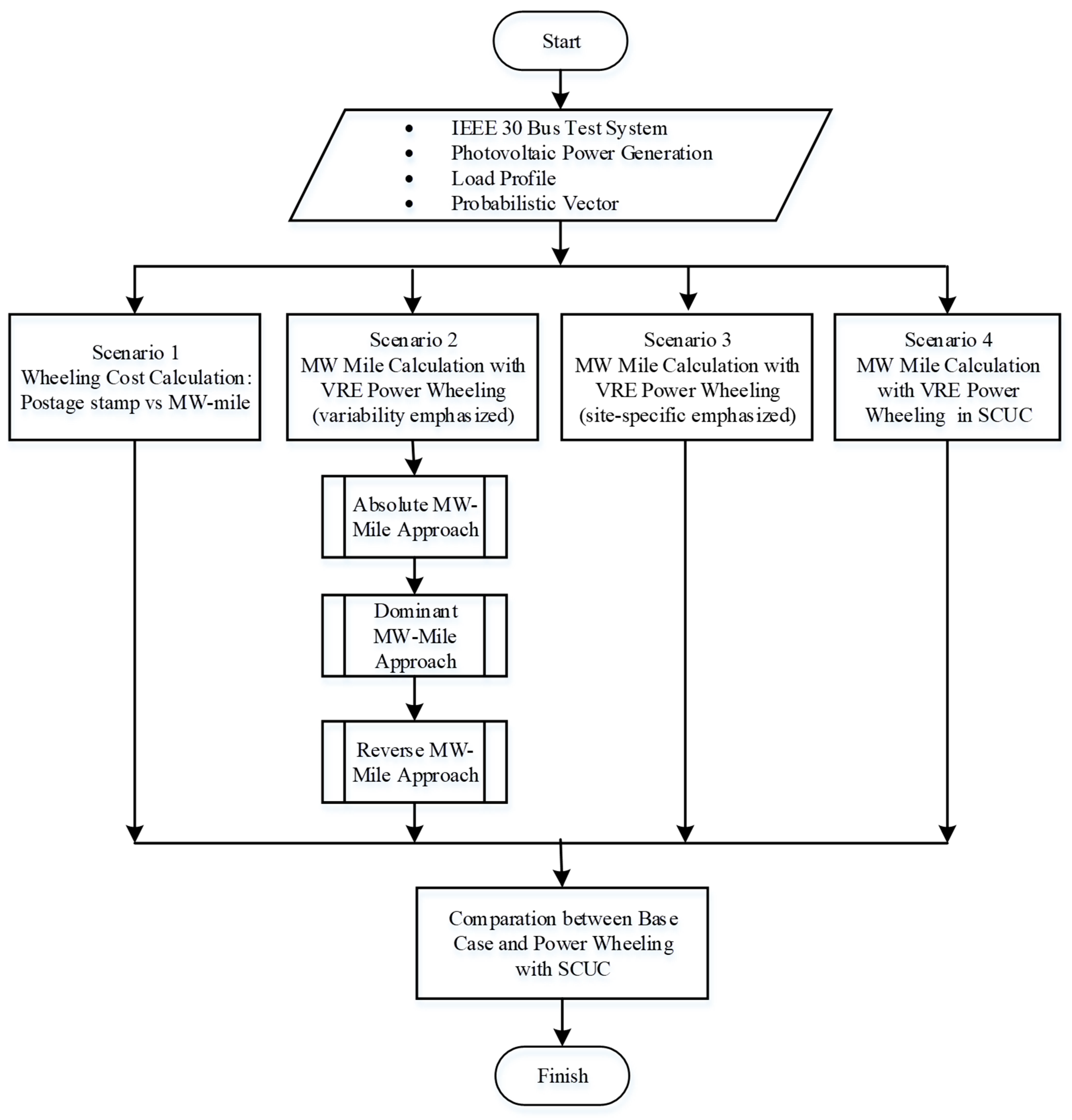
This research was carried out using the flowchart shown in Figure 1. The research began with inputting data for the calculation of the baseline unit commitment and OPF. The results of these calculations were then used as the basis for calculating the cost of power wheeling using the MW mile method based on power tracing. After the baseline was obtained, the next stage of calculation was carried out by entering a contingency scenario to obtain the cost of power wheeling that considers the security-constrained unit commitment (SCUC). There are four scenarios studied in this paper: (i) wheeling cost calculation: postage stamp vs. MW mile, (ii) MW mile calculation with variability-focused VRE, (iii) MW mile calculation with site-specificity-focused VRE, and (iv) MW mile calculation with contingency-focused VRE. The first scenario aimed to provide a general concept of the power wheeling cost calculation by comparing the MW mile method with the postage stamp method, which is considered the conventional wheeling method. The second scenario aimed to investigate the impact of the variability of the VRE and the most suitable MW mile method by calculating the cost using three methods: absolute, dominant, and reverse. The most suitable MW mile method will be used for scenarios three and four. The third scenario investigates the impact of the site specificity of the VRE. The fourth scenario compares the final cost of power wheeling should contingency happen.
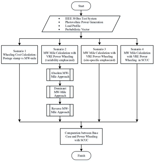
Figure 1.
Research flowchart.
3. Network and Test Cases
This section presents the employed network, the modified IEEE 30 bus test system, and test cases performed to assess the impact of VRE and contingency in the network.
3.1. Modified IEEE 30 Bus
The IEEE 30 bus was selected as the base test network for this research as it has been used primarily for planning studies [31]. The IEEE 30 bus is also a well-known method network with sufficient complexity, i.e., not too simple or complex; hence, studied phenomena will occur but not be overshadowed by the grid strength. Two sensitivity analyses have also been conducted on the IEEE 30 bus [32,33], which prove pivotal for selecting understudied nodes in the IEEE 30 bus in this research. The modification of the IEEE 30 bus is in the form of adding three photovoltaic plants at buses 4, 5, and 18 with generation values of 12 MW, 25 MW, and 100 MW, respectively. The modification also included additional loads at buses 19, 24, and 6 with load values of 8 MW, 20 MW, and 90 MW, respectively. The IEEE 30 bus single line modification diagram and its transmission line data can be seen in Figure 2 and Table 1, respectively [34,35].

Figure 2.
Modified IEEE 30 bus system.

Table 1.
Line cost.
3.2. Daily Loading and VRE Profile
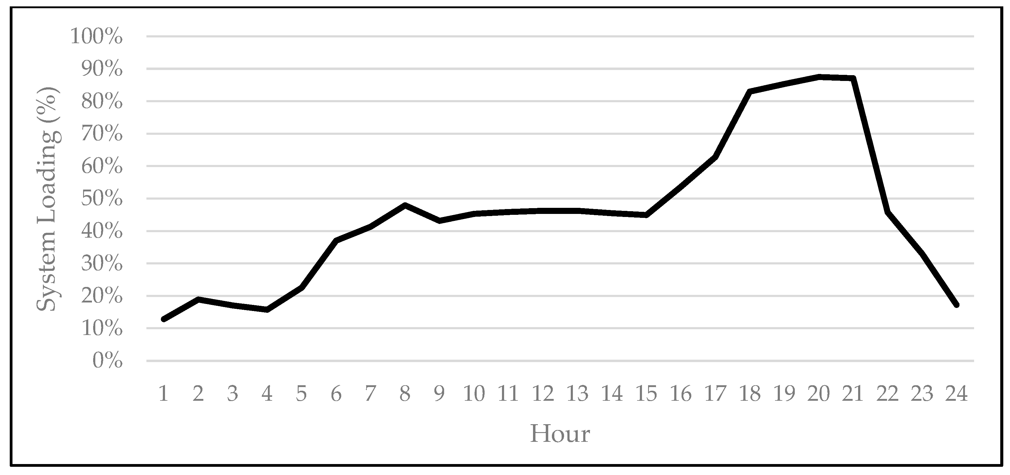
The simulation is performed in a 24 h multi-period OPF. Each period was assumed to represent the duration of system operation for 1 h. An inter-period transition in the form of transition probability is considered. i.e., system state (system loading, generation profile, generator’s ramping profile, variability of VRE, and other variables) at hour t is taken into account and affects the system state at t + 1. This means that the actual load profile at hour t at different loads will slightly differ from its base load profile (shown in Figure 3) and from each other. This modeling approach is aimed at providing a more realistic depiction of a real system where loads follow the load profile but with hourly and/or daily variation. This process is conducted in the MOST package.

Figure 3.
System load profile.
In terms of power wheeling actors, there are three actors (VRE owners) in the form of the photovoltaics modeled in this research. The generation profile of the VRE follows the irradiance profile based on data from the photovoltaic geographical information system (PVGIS) [36,37]. The data were processed via the system advisor model (SAM) [38] software (Version 2020.11.29) to obtain an estimate of electricity production. The generating capacities of power wheelers 1, 2, and 3 are 12 MW, 25 MW, and 100 MW, respectively. The generator locations belonging to the power wheeling actors 1, 2, and 3 are on buses 4, 5, and 18. It is worth noting that the VRE generation is prioritized over the non-VRE generator, i.e., all the VRE generation will be exported to the grid.
3.3. Study Cases
There are four study cases performed in this paper, created from a combination of VRE, unit commitment, and SCUC presence. These four study cases are shown in Table 2. The first case was used as a baseline for calculation. The second study case aimed to investigate the impact of the site variability of VRE on the wheeling cost, while the third case was simulated to investigate the impact of VRE site specificity on the wheeling cost. The third case is addressed to identify the impact of contingency on wheeling costs. The contingency scenario is displayed in Table 3, where a set of network events, namely branches 14–15 and branches 6–10 out of service, are performed. It is worth noting that each event is independent and has a different probability of occurring. A probabilistic contingency event is performed for each simulated hour.
Table 2.
Four study cases were performed in this simulation.
Table 3.
Contingency scenario.
4. Result and Discussion
This section contains four subsections, with the first section aiming to elaborate on the power wheeling concept by adding three synchronous generators and calculating the cost based on two wheeling methods: postage stamp and MW mile. The second and third subsections aimed to investigate the impact of the variability and site-specificity of VRE. The last subsection aimed to provide deeper insights into the power wheeling concept by introducing contingency events in the form of line disconnection and generator derating.
4.1. Impact of Power Wheeling on Existing Power System Operation
The impact of power wheeling on the system is investigated by introducing three new unit commitment synchronous generations in the IEEE 30 bus system.
In the first study case, the system is modeled over 24 h periods, with details of the modeling (including the rating of the three generators) provided in Section 3. The impacts of these three new generators are observed based on the generators’ unit commitment, line loading, and the resulting power wheeling cost. The results of the unit commitment before and after the successive 24 h periods can be seen in Table 4 and Table 5. It is worth noting that the generator that has a different unit commitment is marked in red. It can be observed that the addition of three new synchronous generators does not significantly change the unit commitment of each generator. This is because the three newly introduced generators are of the same type; subsequently, their cost functions are the same. Thus, the change in the power flow only takes loss minimization into account.
Table 4.
Unit commitment from the system without power wheeling for the 24 h period.
Table 5.
Unit commitment from the system with non-VRE power wheeling for the 24 h period.
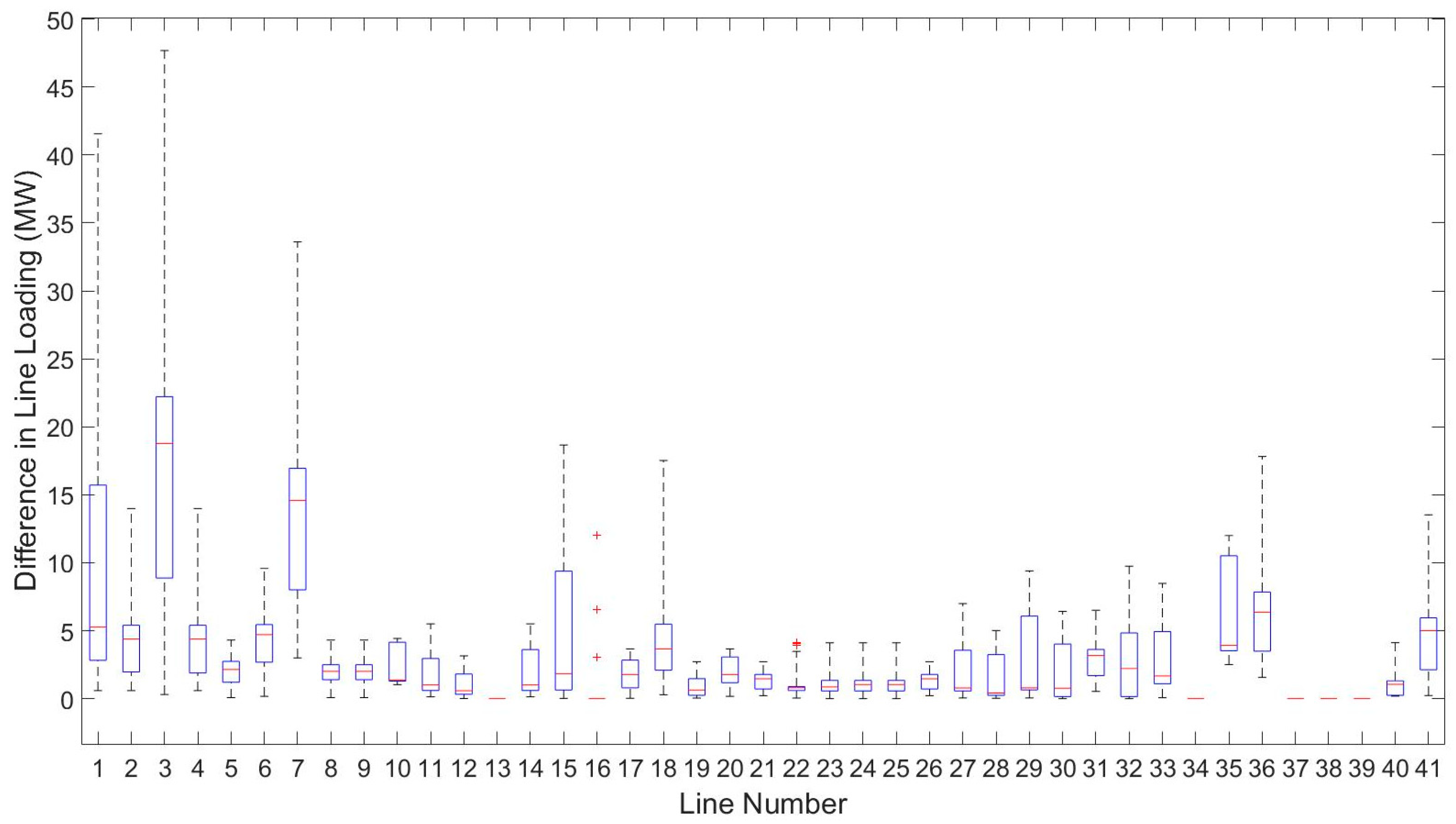
The result from the 24 h simulation based on Table 4 and Table 5 is presented in the form of a boxplot of the line loading difference shown in Figure 4. It can be seen that due to the presence of non-VRE generators (generators 7, 8, and 9), power flow and therefore line loading are changing significantly. The highest change in terms of line loading is on line number 7, where it connects bus numbers 4 and 6. In the new configuration, bus 4 is installed with a non-VRE generator of 12 MW, whereas bus 6 is installed with a non-VRE generator of 90 MW. Hence, the addition of two non-VRE generators explains why line 7 has the highest variability in terms of boxplot. Note that for line numbers that possess little to no difference in terms of variability (denoted by a red stripe), such as lines 37–39, those are lines connecting buses 27, 28, 29, and 30. Those buses are located furthest from the newly installed non-VRE generators, which explains why those lines do not have any loading changes.

Figure 4.
Difference in line loading between non-VRE power wheeling and existing conditions. The + sign represents outlier whereas the (double) − sign represents whisker. The whiskers are the two lines (denote with − sign) outside the box, that go from the minimum to the lower quartile (the start of the box) and then from the upper quartile (the end of the box) to the maximum. An outlier is defined as a data point that is located outside the whiskers of the box plot.
Figure 5 shows a comparison of the cost of power wheeling for calculations with two methods: the postage stamp and the MW mile. As elaborated in Section 2, the postage stamp does not pay attention to real network usage or system operation; this method only pays attention to the energy consumed via the load. It is assumed that all the power generated via the power wheeling generator is entirely channeled and consumed via the power wheeling load. Based on the line cost value in Table 1, it is known that the energy distribution cost is USD 0.61 kWh. Since the postage stamp only pays attention to the amount of energy consumed via the power wheeling load, the power wheeling costs will be proportional to the energy consumption of each power wheeling load. The cost of power wheeling using postage stamps for these 24 h periods is displayed in Figure 5a. As shown in the figure, power wheeling actor three has the highest cost because it has a load of 90 MW. The total cost of power wheeling charged for the 24 h periods is USD 5911.82. The cost of power wheeling for actors 1 and 2, respectively, is USD 525.50 and USD 1313.74 for operations over these 24 h periods.
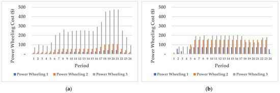
Figure 5.
Power wheeling costs for non-VRE in (a) the postage stamp method and (b) the MW mile method.
On the other hand, the MW mile method considers network usage and system operation by power wheeling actors. Thus, the costs incurred will be based on how big the impact of the power wheeling is on the system. The reference for identifying network usage and operating impact on the system is from the side of the generator’s power wheeling. The identification of network usage via power wheeling actors is based on tracing calculations. The power wheeling actors will only be charged according to the network on the system they use. Figure 5b shows the cost of power wheeling for the three power wheeling actors. The tracing results show that in period one, power wheeling actors one and three did not use the network because, at that time, the two power wheeling generators were not operating. The same happened to power wheeling generator two in period three, power wheeling generators one and two in period four, and power wheeling generator three in a 24 h period. It can be concluded that effective power tracing can identify network usage when implementing power wheeling. Power wheeling actors will only be charged according to the network they use. Thus, calculating power wheeling using power tracing-based MW miles provides a better level of fairness than the postage stamp method.
4.2. Impact of Variability of VRE on Power Wheeling Cost
Power wheeling with a dispatchable power plant, i.e., a synchronous generator, allows the existing system to include it in the generator scheduling. Should a non-dispatchable generator, i.e., a VRE without battery, be used, the power flow, line loading, and power wheeling costs will be different. Generator scheduling due to the inclusion of power wheeling with VRE generators can be seen in Table 6. As shown in Table 6, the use of a VRE generator as a power wheeling generator in this simulation causes a change in the generator schedule in the existing system. These changes occurred in generators one (in periods six and twenty-three), two (in periods one to four), and five (in period twenty-four).
Table 6.
Unit commitment from the system with VRE power wheeling for the 24 h period.
The implementation of power wheeling with VRE also causes a change in line loading in the existing system. Figure 6 shows the average load change for each line over a period of 24 h if the power wheeling generator changes from a non-VRE generator to a VRE generator. The three lines with the biggest changes occurred on lines one (line bus one to bus two), two (line bus one to bus three), and four (line bus three to bus four). This happened because of a change in the supply from generator one, which functions as a swing. This change in the supply from generator one is due to the power requirements of the system being assisted via the inclusion of G7, G8, and G9.

Figure 6.
Difference in line loading between non-VRE and VRE power wheeling. the + sign represents outlier whereas the (double) − sign represents whisker. The whiskers are the two lines (denote with − sign) outside the box, that go from the minimum to the lower quartile (the start of the box) and then from the upper quartile (the end of the box) to the maximum. An outlier is defined as a data point that is located outside the whiskers of the box plot.
Power wheeling in the existing system also causes a change in the direction of power flow. Figure 7 shows the number of lines that experience changes in the direction of power flow in each period. The period that has the greatest number of changes in the direction of power flow is period 38. This is a transitional period of significant loading changes based on the load profile. During this period, there was also a change in the composition of the generation because the VRE generators were no longer in production. The changes in the flow direction of each line in each of these periods can be further identified. The results of this identification can be used as a basis for calculating the costs of power wheeling. If the power flow due to power wheeling is opposite to the power flow in the existing conditions, it will reduce the load on the line. This will ultimately reduce losses down the line.

Figure 7.
Number of line changes per period.
The calculation of the cost of power wheeling with the VRE generator is carried out using four methods. The comparison of the cost of power wheeling for each actor in each period based on the four methods is shown in Figure 8. Calculations using the postage stamp method do not pay attention to network utilization or aspects of system operation. Thus, the type of generator used in power wheeling will also not affect the calculation.

Figure 8.
Power wheeling cost for VRE in (a) the postage stamp method, (b) the absolute MW mile method, (c) the dominant MW mile method, and (d) the reverse MW mile method.
The type of generator used for power wheeling in this scenario is a VRE generator with a photovoltaic type without batteries. Therefore, the power wheeling plant will only be in production during the day. The power wheeling load will be supplied by the utility generator when the power wheeling plant is not operating. Power wheeling operations technically do not occur when the power plant is not operating. This condition is not considered in the calculation of power wheeling with the postage stamp method. Thus, there will be a condition where power wheeling does not occur, but the power wheeling actor still has to pay a fee.
Should the MW mile method be used instead of the postage stamp method, power wheeling actors will only be charged according to the line used and according to the impact on system operation. Figure 8b shows the cost of power wheeling using the absolute MW mile method. With this method, power wheeling actors are not burdened with costs when their generator is not operating. The absolute MW mile method is combined with the power tracing method so that the lines affected by each power wheeling actor can be identified. Figure 8b shows that power wheeling actor generator one is the power wheeling agent that influences the line the most. This causes it to bear the highest power wheeling costs even though it has the smallest capacity. On the other hand, power wheeling actor three, which is the power wheeling actor with the largest capacity, actually has the lowest cost, a total of USD 935.91 for a power wheeling capacity of 90 MW for 24 h. This is because the perpetrators of power wheeling affect the line the least. The generator of power wheeling actor three tends to supply the surrounding loads, so it does not use a lot of lines. Because power wheeling only utilizes the remaining capacity of the line in the system, power wheeling actors do not need to be burdened with the investment costs of the line.
The absolute MW mile method does not pay attention to the direction of power flow caused by power wheeling actors. The MW mile method that pays attention to the direction of the power flow for power wheeling actors is the dominant MW mile method, as are the reverse MW mile methods. The calculation of the cost of power wheeling with the dominant MW mile method is shown in Figure 8c. The results of the reverse MW mile method are shown in Figure 8d. The calculation results show the same pattern, namely successive power wheeling actors from the highest cost to the lowest cost: power wheeling actors one, two, and three. The same thing also happens in the reverse MW mile method. This is inversely proportional to the capacity of power wheeling actors; power wheeling one actually has the smallest capacity value, and power wheeling three has the largest capacity. The absolute MW mile is the best method from the perspective of network asset ownership because this method provides certainty in the process of leasing network assets as the transmission line owner receives compensation for any power flowing through their asset. Based on the system operator’s perspective, the absolute MW mile method is also easier to quantify compared to the other two methods. The drawback of this method, specifically the higher total cost, can be mitigated by proportionally adjusting the line cost. Therefore, the electricity price charged to the customer remains fair. Based on these reasons, the absolute MW mile method will be used in the next subsection.
4.3. Impact of Site Specificity of VRE on Power Wheeling Cost
The next simulation scenario is to change the location of the power wheeling generators. All power wheeling generators are placed on the bus closest to their respective load buses. This location change affects the scheduling of the utility’s generator. As much as 36.8% of the utility’s generator scheduling status changed. The unit commitment of the power plant belonging to the utility after the relocation of the power wheeling plant location is shown in Table 7.
Table 7.
Unit commitment from the system with VRE power wheeling with location change.
The change in location of the power wheeling generator also causes a change in line loading. The average change in the loading of all lines for the 24 h periods can be seen in Figure 9. As shown in Figure 9, there has been a relatively large change in the loading compared to the previous scenarios. The biggest change in loading occurs on line one. This line connects bus one to bus two. On buses one and two, there is a generator belonging to the utility.

Figure 9.
Difference in line loading in VRE power wheeling with location change.
The power wheeling costs for this scenario are then compared with the cost yielded in the previous section, i.e., the impact of the variability of VRE. It is worth noting that both results were calculated using the absolute MW mile method. The calculation results of the site-specificity impact of VRE are presented in Figure 10b, where they show a decrease in costs for power wheeling actors one and two. However, the cost of power wheeling for three actors increases. This implied that, compared to variability, the site specificity of VRE is more sensitive to the power wheeling cost, as the cost is heavily affected by the line used by power wheeling actors, i.e., there are cheap and expensive lines. The impact of line cost is then further studied in the next section with the introduction of line contingency events, where the selection of lines used by power wheeling actors is limited.

Figure 10.
Power wheeling cost with the MW mile absolute method for VRE with location change (a) before location change (variability) and (b) after location change.
4.4. Impact of Contingency on Power Wheeling Cost
The next scenario is one that includes the contingency aspect. The utility’s generator scheduling in this condition can be seen in Table 8.
Table 8.
Unit commitment from the system with VRE power wheeling and contingency.
As shown in Table 8, the applied contingencies cause changes to generator scheduling. Of the 144 generator statuses, there were 31 that experienced changes of 22%. This change in generation status also has an impact on online loading. The average line change during this contingency is shown in Figure 11. In the figure, the average change in loading for the entire period on each line is evident. The three lines that experienced the biggest changes were lines one, three, and seven.

Figure 11.
Difference in line loading in VRE power wheeling with contingency. the + sign represents outlier whereas the (double) − sign represents whisker. The whiskers are the two lines (denote with − sign) outside the box, that go from the minimum to the lower quartile (the start of the box) and then from the upper quartile (the end of the box) to the maximum. An outlier is defined as a data point that is located outside the whiskers of the box plot.
Cost calculation in this condition is carried out using absolute MW mile. The cost of power wheeling is compared between the costs before the contingency occurs and the costs after the contingency occurs. The comparison of the costs for the two conditions can be seen in Figure 12.

Figure 12.
Power wheeling cost with the MW mile absolute method for VRE with contingency (a) before contingency and (b) contingency condition.
The calculation results show that the cost of power wheeling when contingencies occur actually yields a lower value. This happened for power wheeling generators one, two, and three. Changes in power flow patterns due to this contingency have caused power wheeling plants to use fewer lines. Therefore, the costs that must be paid by the power wheeling actors are also lower. Based on the four scenarios, the difference in power wheeling cost compared to the conventional postage stamp method is presented in Table 9.
Table 9.
Difference of power wheeling actors for different scenarios compared to postage stamp.
As shown in Table 9, actor one experiences a significant increase, while in general, actors two and three experience a decrease in costs. These are attributed to the transmission segment used by each actor and the cost of transmission usage in each line. Table 10 provides a better context to understand the impact of transmission usage and its cost on the total power wheeling cost. As shown in Table 10, most of the power wheeling cost from actor one is due to the usage of lines 2–4, where the cost per km is 509.950 and its length is 278 km.
Table 10.
Breakdown of used lines, cost of lines, and length for each actor from Table 9.
5. Conclusions, Recommendations, and Future Work
This paper presents research focused on the impact of the variability and site specificity of VRE on power wheeling costs. The implication of contingencies on the power wheeling cost is also assessed in this research. A meshed network in the form of a modified IEEE 39 bus, due to its suitability for planning studies, is employed in this research. The wheeling cost is calculated using the postage stamp and MW mile methods. The postage stamp method ignores transmission system utilization, whereas using the MW mile is a method that focuses on the trajectory and amount of power flowing from one generator to the loads. It is assessed and proven via simulation that the MW mile is fairer than the postage stamp method in terms of power wheeling cost calculation.
Further conclusions derived from the research on VRE impact on power wheeling costs are as follows:
- Variability is less sensitive towards power wheeling cost calculation as the cost is heavily affected by the line used by power wheeling actors, i.e., a 100 MW power flow through the line with a total cost of USD 1/MW will be cheaper compared to a 50 MW power flow through the line with a total cost of USD 2.5/MW;
- Site specificity is critical for power wheeling cost calculation as it affects the power flowing through specific lines, i.e., there are cheap lines as well as expensive lines;
- Line contingency results in a lower power wheeling cost as power wheeling actors use fewer and cheaper lines. This is possible due to the use of meshed networks.
Based on the findings, it is recommended for utilities to implement the power wheeling concept using the MW mile method instead of the postage stamp method for VRE generators. A fair power wheeling cost calculation also needs to incorporate the site specificity and variability of VRE and consider the probability of line contingency. It is worth noting that this study only compares two types of power wheeling methods and uses a test-case system. Therefore, in the future, the authors want to propose a novel power wheeling method and apply it to an actual network, such as the Indonesian system. An application to the Indonesian system will help the Indonesian power system utility structure the power wheeling cost scheme and relevant policies.
Author Contributions
Conceptualization, Y.S.W.; Methodology, Y.S.W.; Writing—original draft, Y.S.W.; Writing—review & editing, S.P.H. and S.; Supervision, S.P.H. and S. All authors have read and agreed to the published version of the manuscript.
Funding
This research was funded by Kementerian Pendidikan, Kebudayaan, Riset, dan Teknologi (089/E5/PG.02.00.PT/2022;1926/UN1/DITLIT/Dit-Lit/PT.01.03/2022).
Institutional Review Board Statement
Not applicable.
Informed Consent Statement
Not applicable.
Data Availability Statement
This Study did not report data.
Conflicts of Interest
The authors declare no conflict of interest.
References
- Mustika, D.P.; Hadi, S.P.; Isnaeni, M.B.; Frasetyo, M.B. Improving Transient Stability in DFIG-Based Wind Turbines Using Bridge-Type SFCL. J. Nas. Tek. Elektro Dan Teknol. Inf. 2022, 11, 297–304. [Google Scholar] [CrossRef]
- International Energy Agency. Net Zero by 2050—A Roadmap for the Global Energy Sector. 2021. Available online: www.iea.org/t&c/ (accessed on 30 July 2023).
- Ministry of Energy and Mineral Resources. Peraturan Menteri Energi dan Sumber Daya Mineral Republik Indonesia Nomor 11 Tahun 2021 Tentang Pelaksanaan Usaha Ketenagalistrikan; 2021. Available online: https://jdih.esdm.go.id/storage/document/ (accessed on 22 June 2023).
- U.S. Energy Information Administration. Levelized Cost and Levelized Avoided Cost of New Generation Resources in the Annual Energy Outlook 2020. 2020. Available online: https://www.eia.gov/outlooks/aeo/pdf/electricity_generation.pdf (accessed on 29 July 2023).
- Kanagaraj, N.; Mollajafari, M.; Mohammadiazar, F.; Akbari, E.; Sheykhi, E.; Chaoui, H. A New Voltage-Multiplier-Based Power Converter Configuration Suitable for Renewable Energy Sources and Sustainability Applications. Sustainability 2022, 14, 16698. [Google Scholar] [CrossRef]
- Huang, Y.W.; Kittner, N.; Kammen, D.M. ASEAN grid flexibility: Preparedness for grid integration of renewable energy. Energy Policy 2019, 128, 711–726. [Google Scholar] [CrossRef]
- Hirth, L.; Ueckerdt, F.; Edenhofer, O. Integration Costs Revisited—An Economic Framework for Wind and Solar Variability. Renew. Energy 2015, 74, 925–939. [Google Scholar] [CrossRef]
- Negahban, M.; Ardalani, M.V.; Mollajafari, M.; Akbari, E.; Talebi, M.; Pouresmaeil, E. A Novel Control Strategy Based on an Adaptive Fuzzy Model Predictive Control for Frequency Regulation of a Microgrid with Uncertain and Time-Varying Parameters. IEEE Access 2022, 10, 57514–57524. [Google Scholar] [CrossRef]
- Saxena, A.; Pandey, S.N.; Srivastava, L. Genetic Algorithm based Wheeling Prices Allocation for Indian Power Utility by using MVA-Mile and MW-Mile Approaches. In Proceedings of the International Conference on Emerging Trends in Electrical, Electronics and Sustainable Energy Systems, ICETEESES 2016, Sultanpur, India, 11–12 March 2016; IEEE: Piscataway, NJ, USA, 2016; pp. 60–63. [Google Scholar] [CrossRef]
- Heeter, J.; Vora, R.; Mathur, S.; Madrigal, P.; Chatterjee, S.K.; Shah, R. Wheeling and Banking Renewable Energy Wheeling and Banking Strategies for Optimal Renewable Energy Deployment: International Experiences. 2016. Available online: https://www.nrel.gov/docs/fy16osti/65660.pdf (accessed on 29 July 2023).
- Zahid, H.; Altamimi, A.; Kazmi, S.A.A.; Khan, Z.A. Multi-phase techno-economic framework for energy wheeling via generation capacity design of microgrids and virtual power plants. Energy Rep. 2022, 8, 5412–5429. [Google Scholar] [CrossRef]
- Saxena, A.; Tripathi, A. Wheeling Prices Methodology: A Review. Int. J. Enhanc. Res. Sci. Technol. Eng. 2014, 3, 196–201. [Google Scholar]
- Li, B.; Robinson, D.A.; Agalgaonkar, A. Identifying the Wheeling Costs Associated with Solar Sharing in LV Distribution Networks in Australia using Power Flow Tracing and MW-Mile Methodology. In Proceedings of the 2017 Australasian Universities Power Engineering Conference, AUPEC 2017, Melbourne, VIC, Australia, 19–22 November 2017; pp. 1–6. [Google Scholar] [CrossRef]
- Larbwisuthisaroj, S.; Chaitusaney, S. Wheeling Charge Considering Line Flow Differentiation based on Power Flow Calculation. In Proceedings of the ECTI-CON 2018—15th International Conference on Electrical Engineering/Electronics, Computer, Telecommunications and Information Technology, Chiang Rai, Thailand, 18–21 July 2018; IEEE: Piscataway, NJ, USA, 2018; pp. 293–296. [Google Scholar] [CrossRef]
- Sahay, S.; Kumar, N.; Joshi, H. Modified MW Mile Method for Pricing the Transmission Services by Including Transmission Losses and Variation in the Load Power Factor. In Proceedings of the 2018 International Conference on Smart Electric Drives and Power System, ICSEDPS 2018, Nagpur, India, 12–13 June 2018; IEEE: Piscataway, NJ, USA, 2018; pp. 267–271. [Google Scholar] [CrossRef]
- Saxena, A.; Pandey, S.N.; Srivastava, L. DC-OPF Based Allocation of Wheeling Prices for Varying Contribution of Producers and Customers. In Proceedings of the 1st IEEE International Conference on Power Electronics, Intelligent Control and Energy Systems, ICPEICES 2016, Delhi, India, 4–6 July 2016; pp. 3–7. [Google Scholar] [CrossRef]
- Yang, Z.; Zhong, H.; Xia, Q.; Kang, C.; Chen, T.; Li, Y. A Structural Transmission Cost Allocation Scheme Based on Capacity Usage Identification. IEEE Trans. Power Syst. 2016, 31, 2876–2884. [Google Scholar] [CrossRef]
- Wongkom, T.; Chaitusaney, S. Wheeling Charge Calculation with Consideration of Investment Lifetime and Power Transaction Locations. In Proceedings of the 16th International Conference on Electrical Engineering/Electronics, Computer, Telecommunications and Information Technology (ECTI-CON 2019), Pattaya, Thailand, 10–13 July 2019; pp. 321–324. [Google Scholar] [CrossRef]
- Fatchurrahman, R.; Zakaria, A.B. Study of Determining Cost Compensation of Power Wheeling Transaction on Composite System Reliability by Optimal Power Flow. In Proceedings of the 2019 International Conference on Technologies and Policies in Electric Power & Energy, Yogyakarta, Indonesia, 21–22 October 2019. [Google Scholar] [CrossRef]
- Abdullahi, A.B.; Olatomiwa, L.; Tsado, J.; Sadiq, A.A. Impact Assessment of Wheeling Renewable Distributed Generation to Residential Load. In Proceedings of the International Conference on Electrical, Computer, and Energy Technologies, ICECET 2021, Cape Town, South Africa, 9–10 December 2021; Institute of Electrical and Electronics Engineers Inc.: Piscataway, NJ, USA, 2021. [Google Scholar] [CrossRef]
- Mukherjee, S. A Hub-and-Spoke approach to Optimizing Energy Wheeling of Renewable Resources. In Proceedings of the 2021 IEEE PES/IAS PowerAfrica, PowerAfrica 2021, Nairobi, Kenya, 23–27 August 2021; Institute of Electrical and Electronics Engineers Inc.: Piscataway, NJ, USA, 2021. [Google Scholar] [CrossRef]
- Orfanos, G.A.; Tziasiou, G.T.; Georgilakis, P.S.; Hatziargyriou, N.D. Evaluation of Transmission Pricing Methodologies for Pool Based Electricity Markets. In Proceedings of the 2011 IEEE PES Trondheim PowerTech: The Power of Technology for a Sustainable Society, POWERTECH 2011, Trondheim, Norway, 19–23 June 2011; IEEE: Piscataway, NJ, USA, 2011; pp. 1–8. [Google Scholar] [CrossRef]
- Lawal, M.O.; Komolafe, O.; Ajewole, T.O. Power-flow-tracing-based congestion management in hydro-thermal optimal power flow algorithm. J. Mod. Power Syst. Clean Energy 2019, 7, 538–548. [Google Scholar] [CrossRef]
- Lalitha, K.H.; Kiran, I.K. Comparison of Wheeling Cost using Power Flow Tracing Methods in Deregulated Electric Power Industry. Int. J. Eng. Technol. Manag. Appl. Sci. 2017, 5, 861–870. [Google Scholar]
- Kirschen, D.; Allan, R.; Strbac, G. Contributions of Individual Generators to Loads and Flows. IEEE Trans. Power Syst. 1997, 12, 52–60. [Google Scholar] [CrossRef] [PubMed]
- Zimmerman, R.D.; Murillo-Sánchez, C.E.; Thomas, R.J. MATPOWER: Steady-State Operations, Planning, and Analysis Tools for Power Systems Research and Education. IEEE Trans. Power Syst. 2011, 26, 12–19. [Google Scholar] [CrossRef]
- Murillo-Sánchez, C.E.; Zimmerman, R.D.; Anderson, C.L.; Thomas, R.J. Secure Planning and Operations of Systems with Stochastic Sources, Energy Storage, and Active Demand. IEEE Trans. Smart Grid 2013, 4, 2220–2229. [Google Scholar] [CrossRef]
- Optimization, L.G. Gurobi Optimizer Reference Manual. 2023. Available online: https://www.gurobi.com (accessed on 30 July 2023).
- Lamadrid, A.J.; Munoz-Alvarez, D.; Murillo-Sanchez, C.E.; Zimmerman, R.D.; Shin, H.; Thomas, R.J. Using the MATPOWER Optimal Scheduling Tool to Test Power System Operation Methodologies Under Uncertainty. IEEE Trans. Sustain. Energy 2019, 10, 1280–1289. [Google Scholar] [CrossRef]
- Yang, N.; Dong, Z.; Wu, L.; Zhang, L.; Shen, X.; Chen, D.; Zhu, B.; Liu, Y. A Comprehensive Review of Security-constrained Unit Commitment. J. Mod. Power Syst. Clean Energy 2022, 10, 562–576. [Google Scholar] [CrossRef]
- UW Electrical Engineering. Power Systems Test Case Archive. Available online: https://labs.ece.uw.edu/pstca/ (accessed on 22 August 2023).
- Divya, B.; Devarapalli, R. Estimation of Sensitive Node for IEEE-30 Bus System by Load Variation. In Proceedings of the 2014 International Conference on Green Computing Communication and Electrical Engineering (ICGCCEE), Coimbatore, India, 6–8 March 2014. [Google Scholar] [CrossRef]
- Totonchi, I.; Al Akash, H.; Al Akash, A.; Faza, A. Sensitivity Analysis for the IEEE 30 Bus System using Load-Flow Studies. In Proceedings of the 2013 3rd International Conference on Electric Power and Energy Conversion Systems, Istanbul, Turkey, 2–4 October 2013. [Google Scholar]
- Al-Roomi, A.R. Power Flow Test Systems Repository; Dalhousie University, Electrical and Computer Engineering: Halifax, NS, Canada, 2015. [Google Scholar]
- González-Longatt, F.M. IEEE 30 Bus Test. 2013. Available online: https://fglongatt.org/OLD/Test_Case_IEEE_30.html (accessed on 1 August 2022).
- European Communities. Photovoltaic Geographical Information System. Available online: https://re.jrc.ec.europa.eu/pvg_tools/en/ (accessed on 6 March 2022).
- Huld, T.; Müller, R.; Gambardella, A. A new solar radiation database for estimating PV performance in Europe and Africa. Solar Energy 2012, 86, 1803–1815. [Google Scholar] [CrossRef]
- National Renewable Energy Laboratory. System Advisor Model Version 2020.11.29 (SAM 2020.11.29). Available online: https://sam.nrel.gov (accessed on 22 June 2023).


Disclaimer/Publisher’s Note: The statements, opinions and data contained in all publications are solely those of the individual author(s) and contributor(s) and not of MDPI and/or the editor(s). MDPI and/or the editor(s) disclaim responsibility for any injury to people or property resulting from any ideas, methods, instructions or products referred to in the content. |
© 2023 by the authors. Licensee MDPI, Basel, Switzerland. This article is an open access article distributed under the terms and conditions of the Creative Commons Attribution (CC BY) license (https://creativecommons.org/licenses/by/4.0/).