Research on Urban Sustainability Indicators Based on Urban Grain: A Case Study in Jinan, China

Abstract

As a concept to describe the characteristics of urban spatial forms, urban grain emphasizes the size of urban parcels. Fine grain and coarse grain are considered essential attributes. Fine grain plays a crucial role in promoting the adaptability of urban development, improving urban vitality, and helping achieve sustainable urban development. Current research on urban grain is scattered and difficult to apply to solve practical urban problems. Therefore, this paper aims to identify the spatial indicators that affect the urban grain, to solve urban problems by adjusting spatial indicators. It contains significant suggestions for improving urban design theory and promoting sustainable urban development. This study primarily uses the comparative method to identify spatial indicators influencing urban grain by comparing coarse- and fine-grain study areas. This study screens relevant spatial indicators (building density, road network density, age of housing structures, building façade width along streets, number of entrances and exits along streets, and function mixture) affecting urban grain through a review and measurements, and it visualizes the representation of spatial indicators using the grid method, determining the correlation between spatial indicators and urban grain. The results show that all six indicators have an impact on urban grain.

1. Introduction

The construction of new cities in China is characterized by fast speed and large scale, which not only makes the appearance of cities highly homogeneous but also brings a series of urban problems, such as insufficient urban vitality and fragmentation of urban culture. The study of urban form contributes to the understanding and analysis of urban development [1]. Urban grain, as an attribute that describes the characteristics of urban form, can likewise be used as a method to analyze urban perspective issues, whose changes are closely related to the evolution of society, economy, culture, and policies. Observing urban problems from the perspective of urban grain helps to analyze the inner changes in cities through the external appearance of urban space.

As a concept to describe the spatial characteristics of cities, urban grain was introduced by Spreiregen in 1965 [2]. Urban grain describes the size of urban parcels (or blocks); coarse grain (large, dispersed parcels) and fine grain (small, clustered parcels) are two essential attribute features in urban planning research and practice. They are also used to describe the clarity or ambiguity of the mixture of different city elements, the variation of which has a critical impact on the urban form. During the early stages of the field, researchers conducted studies on urban grain in their respective fields and gradually refined the concept of urban grain. Spreiregen pointed out that depending on the size of the urban parcel, there are two states of urban grain: coarse-grain and fine-grain [2]. To further refine the theory of urban grain, Kevin Lynch proposed that in addition to coarse-grain and fine-grain, cities also possess clear and ambiguous properties. Clarity is determined by the presence or absence of transitions between two adjacent elements in the same region and proposes the concept of non-physical elements such as temporal and active grain [3]. Jacobs proposed that fine grain boosts the urban economy [4]. Then, researchers emphasized the impact of urban grain on urban form and proposed that urban grain is a scaling relationship between urban blocks and block constituents [5,6,7]. Furthermore, many researchers emphasized urban grain’s non-physical morphological dimension elements, such as parcel function, and gradually clarified urban grain as a professional perspective for urban form studies [8,9,10,11,12,13].

Researchers believed that fine grain positively affects urban development, while coarse grain negatively affects cities. Some researchers believe fine grain improves urban adaptability and sustainability [13,14,15,16], which is reflected in the following five aspects: (1) Some authors argue that fine grain promotes the functional diversity of cities so that the employment and service demands can be served locally [5,7,9,10,14,15]. Furthermore, it is believed to promote the development of intimate relationships between firms, increase firm aggregation, and promote the growth of local firms [15,17]. (2) It has been argued that fine grain can promote the mixture of ownership, which can effectively promote the upgrading of real estate and the number of small-scale investments, increase the proportion of local independent businesses [18,19], create more jobs [17], and enhance the local economy [20]. (3) The third positive effect is fine grain’s ability to promote urban economic development, and some researchers argue that fine grain helps to achieve business diversity [19,21,22], thus reducing the impact of market volatility. Many authors argue that the economic boost of fine grain subsequently provides business activity throughout the day [2,23,24]. (4) Many researchers claim that fine grain improves the aesthetic quality of streets and open spaces by creating attractive streets and spatial features [11,15,25], making architectural groups more harmonious [26] and enhancing the sense of individuality of streets [11,19,27]. (5) Loci pointed out that fine grain helps to enhance street dynamics [25]. Early related theories were enriched by the perspectives of the urban grain concept and its influence on urban development. In order to further play a role in guiding urban planning, some researchers have explored the factors that impact urban grain from multiple perspectives. In addition, the element of urban grain that most intuitively contributes to sustainable urban development is the fact that fine grain is beneficial in increasing the adaptability of urban development. Conzen has suggested that urban parcels change over time due to urban development and that individual buildings in a fine-grain area are less likely to affect their urban surroundings. They can continue to regenerate themselves so that the design of individual plots can gradually intervene in the urban form to increase the resilience of urban development. The closer functional distribution of fine-grain areas reduces vehicle use, which in turn reduces carbon emissions and aids in the development of sustainable cities.

Although most scholars believe fine grain has a positive effect on urban development while coarse grain is detrimental, coarse grain also has some positive effects. Coarse-grain areas tend to have higher urban densities, providing the city with large areas of green or public open space, giving residents more opportunities to interact. In addition, coarse-grain areas are usually large and high-density, which aids in the internal management of the area.

Numerous researchers have suggested that fine grain contributes to solving urban problems to achieve sustainable urban development and believed that elements such as streets [8,28,29,30,31,32,33,34,35], building and population density [2,3,13,36], building age [29,37], natural environment [35,38], real estate development [3,9,35,36,39,40,41,42,43], industrial structure [14,35], policies [8,35,43], construction techniques [43], heritage preservation, and historical culture [3,8,9,10,12,29,43] have an impact on urban grain. However, since the influencing elements involve various aspects such as social history and culture, there are fewer studies on quantifiable spatial indicators of urban grain, so it is not easy to directly guide urban planning practices. This research team has projected a sustainable approach to small-town development from a quantitative analysis and studied the impact of functional distribution and functional aggregation on urban form [44,45,46]. To clarify which spatial indicators could be adjusted to achieve fine-grained areas for sustainable urban development, in this study, we first screened out the relevant spatial indicators affecting urban grain through a literature review. Secondly, we selected coarse- and fine-grained study areas of similar sizes in Jinan, and measured and visualized urban grain size and spatial indicators using the grid method. Finally, we used urban grain as a dependent variable to compare the values of spatial indicators to determine the indicators that have an impact on urban grain. The correlation between indicators and urban grain was judged. The study results showed that the six indicators—building density, road network density, age of housing structures, building facade width along streets, number of entrances and exits along streets, and function mixture—all impact urban grain.

2. Methodology

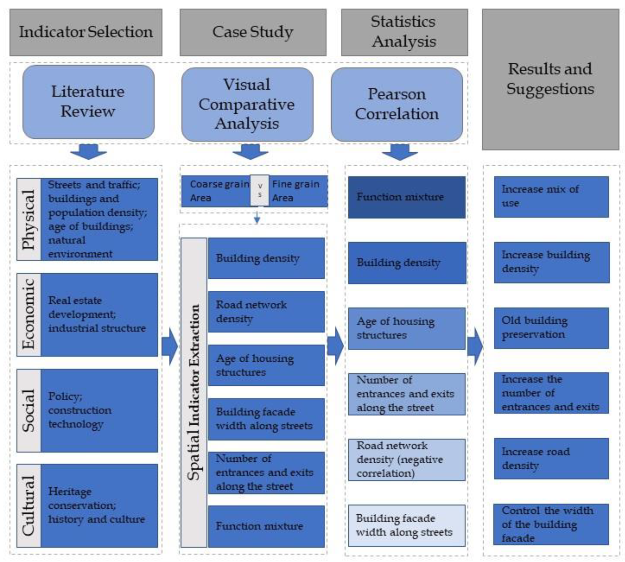
This study used a case study approach to achieve the research objectives, in which the city research method was used to obtain data for the study and the quantitative analysis method was used to determine the relationship between each indicator and urban grain. In the first phase (Figure 1), urban grain’s spatial indicators were identified based on a literature review, which provided the basis for determining the content of the study. In the second stage (Figure 1), the study areas included Jinan Shangbu (fine grain) and Tangye New District (coarse grain), and experimental data were acquired using open-source data in combination with urban research. In the third stage (Figure 1), a data analysis was performed. Additionally, a visual graphical comparison of spatial indicators between the coarse- and fine-grained study areas were carried out, and finally, the relationship between urban grain and spatial indicators was analyzed to determine the spatial indicators of urban grain.

2.1. Spatial Indicator Extraction

The research objective of this study was to identify the spatial indicators that influence urban grain and to regulate these indicators to change urban grain and, thus, promote sustainable urban development. Therefore, it was necessary to screen and transform the factors into quantifiable and modifiable spatial indicators. A total of 32 papers related to urban grain indicators were screened in a literature review. Previous research has identified physical factors affecting urban grain, including streets and traffic, density, building age, and the natural environment. The literature on streets and traffic indicates that the division of streets affects the framework of a city and that shorter streets with higher intersection regularity can bring fine grain; road network density is the reason behind this phenomenon. It has been proposed that the average building facade width of streets in fine-grained areas is shorter, increasing the visual richness of the streets [17,20]. Therefore, building facade widths along streets represent a spatial indicator. In addition, the literature indicates that areas with low building density have greater spacing between buildings and are, therefore, less easily formed into a fine grain. The literature on building age points out that areas with old buildings are generally self-built, occupy smaller regions, and are more finely divided; thus, the age of housing structures serves as a regulating indicator for urban grain. The natural environment is mainly related to natural disasters and patterns, which are difficult to regulate and, therefore, are not considered a spatial indicator.

In addition, economic, social, and cultural factors were translated into quantifiable physical indicators. Among the literature on real estate development and industrial structure, the division of land parcels by function was proposed, and large-scale blocks with a single function led to the disappearance of fine grain. Therefore, a land-use mix describing the degree of mixing of land-use types and functional attributes within a given urban block [47] was used to convert the index. In addition, the number of use units in large-scale parcels is low due to single industrial structures, which can be reflected in the spatial factors, as the number of external entrances and exits of buildings is reduced; thus, the economic factors were converted into numbers of entrances and exits of buildings along streets. The literature on policies indicates that policy formulation fundamentally impacts urban grain. Therefore, the physical factors that influence urban grain size (road network density, building density, etc.) can all be used as spatial indicators for their transformation. The literature on construction technology indicates that technological advances have made large-scale buildings possible, thus contributing to coarse grain generation. Additionally, the older the building, the more backward the construction technology, thus showing that construction technology is related to a building’s age, translating it into an indicator for the age of a housing structure. Similarly, the literature on history and culture indicates that the legacy of history and culture creates a particular preference for building scale and road network density. The literature on heritage conservation suggests a preference for preserving old buildings with historical value, which are usually small in scale due to technical constraints; thus, cultural elements could be translated into building density, road network density, and the age of housing structures.

In summary, the spatial indicators were identified as road network density, building density, age of housing structures, building facade width along streets, number of entrances along streets, and function mixture (

Table 1. Spatial index extraction based on literature review (source: author).

Classification of Factors	Urban-Grain-Influencing Factors	Number of Studies	Sources	Spatial Indicator Extraction
Physical factors	Streets and traffic; buildings and population density; age of buildings; natural environment	11	[2,3,13,28,29,30,31,32,33,34,36,37,38]	Building density; road network density; housing age structure; building facade width along the street
Economic factors	Real estate development; industrial structure	10	[3,9,14,35,36,39,40,41,42,43]	Function mixture; number of entrances and exits along the street
Social factors	Policy; construction technology	4	[8,35,43]	Building density; road network density; housing age structure
Cultural factors	Heritage conservation; history and culture	7	[3,8,9,10,12,29,43]	Building density; road network density; housing age structure

) based on relevant and related research, which is assumed to be correlated with urban grain and analyzed empirically.

2.2. Data Analysis Method

The Conzen School emphasizes the following two basic approaches for studying urban form: a synchronic analysis based on a geometric analysis, and a diachronic analysis based on historical maps [48]. The synchronic analysis also emphasizes the analysis of the relative positions, contour scales, and arrangements of morphological elements within a city, which could then be grouped into different categories. The diachronic analysis emphasizes the comparative analysis of the process of change in the morphological elements in a city over time, which can then help determine the temporal relationship of the change in morphological growth. In this paper, a synchronic analysis was mainly utilized to compare two different grain-size areas over the same period to explore the spatial elements affecting grain size.

Norton argued that the research object of urban grain is the parcel [8]; however, since urban grain’s spatial indicators contain multiple scales, such as building density, the width of a building facade along a street, and age structure, they are indicators at the level of building units. The number of entrances and exits are indicators at the block level, and the suitable research object will be selected according to the scale of the urban grain’s spatial indicators. Ding argued that urban fabric forms can be roughly divided into buildings, parcels, and blocks [49], and urban grain is one of the elements that makes up urban fabric and can be analyzed using these three scales. Therefore, in this study, buildings, parcels, and blocks were selected as the research objects according to the scales of spatial indicators.

In this study, the grid system consists of analysis cells applied to integrate the relationship between people, land, function, transportation, and architecture. Previous research suggested that a grid scale of 50 m × 50 m in size could express the relationship of parcels in this study area; thus, this scale was chosen as the analysis cell of the study. Urban grain value was chosen as the dependent variable, which was used to observe how spatial indicators impact urban grain.

Firstly, the dependent variable of urban grain was analyzed. According to the definition of urban grain, the coarseness of urban grain was determined by calculating the number of intersection points of parcels in each grid [8]. Consequently, the input vector data of the parcels in the study area were input into Arc GIS 10.2, after which the urban grain attributes of the parcels were connected to the grid by a spatial join, and the number of parcels in each grid was counted and visualized.

Subsequently, an analysis of the spatial indicators was performed. The first spatial indicator was building density. The building density indicator represents the kernel density of a building. The analysis consisted of importing a building’s base map of the study area in Arc GIS, extracting the building’s center points, and calculating their kernel density. Subsequently, the raster data of the kernel density to the center points of the 50 m × 50 m grid were extracted, and a spatial connection of the points to the grid was performed and visualized. In addition, the bandwidth (search radius) for calculating the kernel density was set to 100 m so that the values of building density could be homogeneously dispersed in each grid [50].

The second spatial indicator was road network density. Similar to building density, road network density was compared by calculating the line density of the study area. The analysis procedure involved a line density analysis of road network data in Arc GIS (the bandwidth was set to 100 m), after which the raster data of line density to the center point of the created 50 m × 50 m grid were extracted and visualized.

The third spatial indicator was the age of housing structures, which was analyzed with the idea of using every ten years as a structural stratum. The number of levels spanned by the unit grid was assigned and visualized for comparison. The analysis involved importing the data in Arc GIS and assigning values according to the ages of the house structures, after which a spatial join between the 50 m × 50 m grid and the ages of the house structures was performed to obtain the number of house-age-graded structures in each grid and visualize them.

The fourth spatial indicator was the width of building facades along the streets. The main research object was the building facade width along the street in each parcel. The value of this indicator was calculated from the width of building facades along the streets in each grid. The analysis procedure involved importing the actual data on building facade width along the streets in Arc GIS (for buildings located at the corner of two roads, the sum of all street facades was entered). Subsequently, the 50 m × 50 m grid was spatially connected to the data for visualization.

The fifth indicator was the number of entrances along the streets. The value of this indicator was calculated using the kernel density of the number of entrances and exits along the block and visualizing it for comparison between the study areas. The analysis procedure involved importing the entrance data along the street area in Arc GIS, setting the bandwidth to 100 m, performing the kernel density calculation, and obtaining a kernel density raster map. Subsequently, the 50 m × 50 m grid center points were extracted, and the values of the raster map were extracted to the grid center points, spatially connected to the grid, and, finally, visualized.

The sixth spatial indicator was function mixture. The research object was to identify the parcel, link the data to the urban parcel attribute table of Arc GIS, make spatial links with the 50 m × 50 m grid to calculate the number of construction land categories in each grid, and visualize them.

In order to verify the relationship, Pearson’s correlation coefficient (Equation (1)) was applied in this study. Generally, Pearson’s correlation coefficient is calculated by dividing the covariance of two variables by the product of their respective standard deviations, and is usually denoted by r. Pearson’s correlation coefficient is a measure of the linear correlation between two variables. The coefficient is widely used in the natural sciences to measure the correlation between two variables and reflects the strength of the linear correlation between them. If the r value is less than 0, it indicates that the two variables are negatively correlated. If the r value is greater than 0, it indicates that the two variables show a positive correlation, and the larger the absolute value, the stronger the correlation. When the r value is equal to 1 or −1, it means that a linear equation can describe the two variables.

$$r_p=\frac{{\displaystyle \sum _{i=1}^N\left(x_i-\overline{x}\right)\left(y_i-\overline{y}\right)}}{\sqrt{{\displaystyle \sum _{i=1}^n{\left(x_i-\overline{x}\right)}^2}}\sqrt{{\displaystyle \sum _{i=1}^n{\left(y_i-\overline{y}\right)}^2}}}$$

(1)

where r_p is the Pearson correlation coefficient; x and y are two variables; and n is the number of samples.

3. Case Study Areas

3.1. Case Study Area Selection

The study area was selected based on the following criteria:

(1)

The urban grain of the selected study area was representative and contrasting (one study segment was a typical coarse-grained area and the other was a typically fine-grained area).

(2)

The data on building density, road network density, age of housing structures, width of the building facades along the streets, number of entrances and exits along the streets, and function mixture in the study area were comparable (it was determined that limiting these variables would have a potential impact on the study results), and the base data were easily accessible.

(3)

The area (1 km²) and the main functional components of the selected study area were similar.

According to previous research, buildings in fine-grained areas are older, while those in coarse-grained areas are often newly built. Therefore, coarse- and fine-grained study areas were selected in typical urban new- and old-building areas, representing the two extreme states in the history of urban development. Currently, most cities are experiencing a dynamic renewal process and are in the intermediate state of mixing coarse- and fine-grained areas; thus, dividing the study area into old and new buildings can represent the two extreme states of coarse and fine grain, respectively. Intercepting this area would generate more comparative, convincing, and scientific data for the study of spatial indicators of urban grain, and the validity of the hypothesis in this area means that most of the urban areas in the intermediate state can be verified as well.

Jinan, as the capital of Shandong Province and a famous historical and cultural city in China, has preserved numerous fine-grained areas with fine and compact parcels during its long urban development process. Additionally, as a political, economic, cultural, scientific, educational, and financial center and an important transportation hub in Shandong Province, the city’s boundaries have expanded rapidly with the rapid economic development in recent years, generating large, coarse-grained areas (Figure 2). The coarse- and fine-grained areas are very contrasting.

The fine-grained study area was selected from the Jinan Shangbu area, opened by the Qing government in 1905 to revitalize commercial development. Many characteristic Chinese and Western buildings have been developed in this area due to the invasion of foreign cultures [51]. The area has a variety of architectural styles, a small scale, and a high density of buildings, making it a precious historical resource in Jinan. In his study, Wang discussed that the Shangbu area is typical of the old city of Jinan [52]. The boundaries of the study area are shown in Figure 3.

The coarse-grained study area was selected from Jinan Tangye New District, located on the rapid development axis of Jinan to the east and belonging to the construction area of demolition planning, with large-scale integration and construction between 2005 and 2015 [53]. The parcels of land are large and scattered. The boundaries of the study area are shown in Figure 4.

3.2. Data Collection

In order to achieve scientific and accurate case studies, the study data were obtained in the following ways:

• Basic satellite maps;
• Documentary information (such as the Jinan City Plan), which can be obtained from the official website of the Jinan Municipal People’s Government and the Jinan Natural Resources and Planning Bureau’s public documents [54,55];
• Surveys, questionnaires, field measurements, etc.

For the accuracy of the data, in addition to satellite maps, field research measurements were conducted and combined with aerial photographs to determine the exact locations of building units, road networks, and entrances and exits along the streets and the widths of building facades along the streets within the study area (Figure 5). The zoning plan map of the study area was also obtained on the official website of the Jinan Natural Resources and Planning Bureau, based on which the vector base map of the parcels within the study area was determined in combination with field research [55] (Figure 5). The functional categories of the parcels were identified based on the classification of urban construction land in China [56]. The age of the buildings was mainly obtained through the survey.

4. Results

4.1. Urban Grain Analysis

First, the results of the urban grain analysis were obtained. There were 141 parcels in the Shangbu study area, while there were only 18 parcels in the Tangye study area. The difference in the number of parcels was significant, and it could be preliminarily determined that the urban grain of the Shangbu area is finer (Figure 6). There were 153 grids with urban grain values of three or higher in the Shangbu study area, while there were only two such grids in the Tangye study area. Compared to the large number of grids with identical and low-scoring grids in the Tangye study area, there were more grids with high scores in the Shangbu area. The mean and maximum values of urban grain in the two areas were calculated separately (

Table 2. Mean and maximum urban grain in the study area (source: author).

Study Area	Number of Grids	Average Value	Maximum Value
Shangbu	439	2.2	6
Tangye	369	1.09	3

), and the two values were 2.2 and 6 in the Shangbu area and 1.09 and 3 in the Tangye area, which means values in the Shangbu area were almost twice as high as those in the Tangye area.

The study results showed a significant difference in urban grain between the two study areas. In the following analysis, the Shangbu study area represents the fine-grained area, and the Tangye study area represents the coarse-grained area by default. This determination criterion was only relative to the two areas in this study.

4.2. Spatial Indicator Analysis

4.2.1. Analysis of Building Density

The Shangbu study area’s building density value was higher (Figure 7). The maximum value of nuclear density in the Shangbu study area (62,260.45) was almost 27 times larger than that in the Tangye study area (2272.42), and even the minimum value was much larger than the maximum value in the Tangye study area.

4.2.2. Analysis of Road Network Density

The following analysis is based on road network density, and the value in the Shangbu study area was higher. There were 308 grids with a road network density above 27.996635 in the Shangbu area, accounting for 70% of the total number of grids in the area. In comparison, there were only 60 such grids in the Tangye study area, accounting for 16% of the total number of grids (Figure 8). Compared to the large number of identical and low-scoring grids in the Tangye study area, there were more high-scoring grids in the Shangbu study area. The two areas’ total and average road network densities were calculated separately (

Table 3. Mean and maximum road network density in the study area (source: author).

Study Area	Number of Grids	Average Value	Maximum Value	Total Values
Shangbu	439	33.254	62.918	14,598.863
Tangye	369	17.635	57.194	6507.269

), and the average value of road network density in the Shangbu study area was 1.8 times higher than that in the Tangye study area. The total density value was 2.2.

4.2.3. Analysis of the Age of Housing Structures

The age of housing structures represents the third spatial indicator, and the age of housing structures in the Shangbu area was more complex (Figure 9). By counting the number of grids in each age structure range (

Table 4. Number of grids and housing age structure value in the study area (source: author).

Housing Age Structure Value Range	Number of Grids in the Shangbu Area	Number of Grids in the Tangye Area
0	13	178
1	189	188
2	148	3
3	54	0
4	24	0
5	7	0
6	2	0
7	1	0
Sum of grids	439	369

), we could see that the age structure of the Shangbu study area was much more mixed, with a maximum value of seven (i.e., there were seven buildings of different age levels in one grid). In contrast, the maximum value of the Tangye study area was only two (three cells).

4.2.4. Analysis of the Width of Building Facades along Streets

The width of the building facades along the streets represents the fourth spatial indicator, and the value of the width of the building facades along the streets in the Tangye study area was more significant (Figure 10). The values were almost all above 50, while the widths in the Shangbu study area were almost all below 50. The average values of the two areas were calculated separately (

Table 5. Mean and maximum building facade width along the street in the study area (source: author).

Study Area	Number of Grids	Average Value	Minimum Value	Maximum Value
Shangbu	439	23.5	3	90
Tangye	369	67.8	14.1	353.5

), from which it could be seen that the average value of the Shangbu study area (67.8) was almost 28 times larger than that of the Tangye area (23.5), and the minimum and maximum values also showed a considerable difference.

4.2.5. Analysis of the Number of Entrances and Exits along Streets

The fifth spatial indicator represents the number of entrances and exits along the streets, and the value in the Shangbu study area was higher (Figure 11). The mean and extreme values of the two areas were calculated separately (

Table 6. Mean and maximum number of entrances and exits along the street in the study area (source: author).

Study Area	Number of Grids	Average Value	Minimum Value	Maximum Value
Shangbu	439	5138.539092	81.859207	13,819.977539
Tangye	369	407.120921	0	3057.429199

). The mean value of the Shangbu study area was almost 12.6 times higher than that of the Tangye study area, and the minimum and maximum values were very different.

4.2.6. Function Mixture Analysis

The last spatial indicator represents function mixture, and the Shangbu area had a higher function mixture (Figure 12). Furthermore, compared with many grids with smaller values along the Tangye area, there were more grids with high values in the Shangbu area (

Table 7. Value and percentage of function mixture in the study area (source: author).

Value of Function Mixture	Number of Grids in the Shangbu Area	Number of Grids in the Tangye Area
0	0	21
1	134	306
2	152	40
3	97	2
4	44	0
5	10	0
6	2	0
Sum of grids	439	369

). About 69.2% of the Shangbu study area’s grids had values above 2, while the Tangye study area only accounted for 11.3% of the total.

4.3. Correlation Analysis of Spatial Indicators and Urban Grain

Pearson’s correlation coefficient was used to determine the correlations, and significant correlations were found between urban grain and the six indicators in the fine-grained study area (

Table 8. Correlation values between urban grain and spatial indicators in the fine grain study area (source: author).

		Urban Grain	Building Density	Road Network Density	Housing Age Structure	Width of Building Facade along the Street	Number of Entrances and Exits along the Street	Function Mixture
Urban grain	Pearson correlation	1	0.335 **	0.138 **	0.314 **	−0.097 *	0.292 **	0.998 **
	Sig. (2-tailed)		0.000	0.004	0.042	0.000	0.000	0.000
	N	439	439	439	439	439	439	439

* Correlation is significant at the 0.05 level (2-tailed). ** Correlation is significant at the 0.01 level (2-tailed).

). When Pearson’s correlation coefficient exceeded zero, the spatial indicators positively correlated with urban grain, meaning that there is a positive correlation between urban grain and building density, road network density, age of housing structures, number of entrances and exits, number of use units, and function mixture, and the higher these indicators are, the finer the urban grain. When Pearson’s coefficient value for the width of building facades was negative, the two were negatively correlated, meaning that the narrower a building facade width is, the finer the urban grain size. The larger the absolute value of Pearson’s coefficient, the stronger the correlation. The six indicators, in descending order of their influence on the relationship of urban grain according to the rating of Pearson’s correlation coefficient values, are as follows: function mixture, building density, age of housing structures, number of entrances and exits, road network density, and building facade widths along the streets.

5. Discussion

The main objective of this study was to identify the spatial indicators affecting urban grain using a comparative analysis to achieve sustainable urban development through urban design. After clarifying the concept of urban grain and the positive impact brought by fine grain, spatial indicators affecting urban grain were extracted, followed by selecting a study area in Jinan, conducting a spatial indicator analysis, and verifying the indicators. The study showed that building density, road network density, age of housing structures, building facade widths along the streets, number of entrances and exits, and function mixture are all correlated with urban grain, among which, except for the negative correlation between building facade width along the streets and urban grain, all other indicators showed a positive correlation, i.e., the larger the value of the indicator, the finer the urban grain.

5.1. Analysis of Study Results

First, the effect of building density on urban grain was investigated. The higher the building density, the closer the distance between two adjacent buildings is, and the higher the likelihood of forming small-scale parcels is. The higher the building density, the shorter the distance between adjacent buildings and the more intensive the urban function are, thus reducing the distance traveled by transportation and reducing carbon emissions. The reason for the role of road network density on urban grain is mainly reflected in the fact that the division of roads affects the framework of the city; thus, shorter streets with crossing regularity contribute to fine grain. In addition, the high mobility of transportation would lead to larger block scales and broader road networks, thus contributing to coarse grain. A house’s age impacts urban grain mainly because the more mixed the age structure of a house is, the more significant the proportion of old buildings is due to construction technology, living habits, and other factors. The scale of old buildings and parcel division was smaller, resulting in fine grain. On the other hand, areas with many old buildings will retain some of their character and become more distinctive over a long period of development, enhancing the urban intent and contributing to the sustainable urban development of the area. The reason for the role of building facade width and the number of entrances along the streets on urban grain is also important, since areas with narrower building facade widths usually have smaller building scales, which contribute to fine grain. Areas with narrower building facade widths are more likely to have a unique street space character than areas with wider building facade widths, which increases the recognizability of the area, attracts people, and enhances the vitality of the area, thus contributing to the development of a sustainable city. Moreover, this allows for more openings to the street (entrances and exits, windows, etc.), increasing the visual diversity while enhancing communication between the street and the interior of a building and enhancing urban vitality. The main reason why function mixture affects urban grain is that in order to meet the needs of the surrounding residents, a functionally rich living circle needs to be formed within a short distance, and small buildings will grow spontaneously with the functional needs, thus contributing to the formation of fine grain. A rich functional diversity reduces the impact of market fluctuations, stabilizes a city’s economy, and promotes sustainable urban development.

5.2. Suggestions for Urban Planning

Based on the above study, efforts should be made to increase the proportion of fine grain in urban construction to ensure sustainable urban development. Specific measures could be implemented in both regulation and design controls.

Increasing the proportion of fine grain requires substantial intervention in the real estate market, housing policies, and zoning controls. Governments play a critical role in this process. This could be achieved, for example, by compulsory purchases, enacting regulations to protect fine-grained areas from destruction, or limiting a certain percentage of small-scale buildings. The 2030 Strategy launched by the NSW branch of the Property Council of Australia (PAC) has specified that 50% of the area along the street of new buildings should be small stores less than 6 m in width [23].

During the visit and research, it was found that the majority of fine-grained areas are concentrated in the undeveloped old city and contain some historical buildings. The government could stimulate the area’s commercial potential by updating and supplementing public service facilities to maximize the preservation of historical buildings while retaining the fine-grained areas.

Design regulation is the most direct way to achieve fine grain, e.g., through planning, design regulation, and renovation of building units. Planning and regulation could increase the proportion of fine-grained areas by refining road networks. A well-connected and dense road network could divide the site into high-density small-scale parcels, thus contributing to fine-grain formation. Therefore, in urban planning, as many bypasses as possible can be designed according to the actual situation to subdivide urban parcels. In addition, retaining a certain percentage of small-scale buildings in planning and design could effectively increase the proportion of fine grain. This can be achieved by controlling the height of buildings, the width of facades, the number of external entrances, etc. The percentage of these small-scale buildings must be calculated to ensure that developers achieve the maximum number of small-scale buildings within a stable revenue range. Increasing the function mixture of a planning area also contributes to fine-grain formation. This primary approach could turn a large area of single-site planning into a mixed-use area to achieve a reasonable ratio of industrial, residential, commercial, and service industries within a particular area to achieve functional fine grain, but also effectively promote the transformation of urban form to fine grain. In addition, the number of entrances and exits could be increased to provide the possibility of independent business in the evening (independent entrances and exits facilitate individual enterprise control of business hours), thus developing the evening economy, realizing a 24 h functional mix, and achieving fine grain in the time dimension.

It is also possible to increase the proportion of fine grain by transforming large-scale building blocks in the following ways: Firstly, building facades could be modified by dividing them to form a narrower building facade width. The primary method to achieve this is to renovate large-scale buildings and enrich large-scale neighborhood spaces. For example, on the outside of the first floor of a large building along a street facade, arranging small buildings with less than 6 m along a street facade can lead to large-scale buildings having smaller and more vibrant spaces to achieve a fine-grained area (Figure 13). In addition, by increasing the permeability of a street through openings in the building facade, the interaction between the street and pedestrians is promoted, thus enhancing the vitality of the street [57]. For example, externalizing some cafes and small stores with unique characteristics increases their transparency on the street. In addition to facade renovation, a building can also be divided in terms of plan dimensions by adding small-scale blocks for different purposes above the roof of large-scale blocks or by adding roof-top parking. Additionally, the Open Building approach proposed by the Dutch architectural theorist Habraken helped realize the creation of fine grain in high-density cities [58], where an architect only designs and builds the supporting part’s basic structure, and the users install and perfect the infill part. This practice could allow buildings to continue to refine their functions through spontaneous growth, thus realizing the refinement of building blocks.

6. Conclusions

The main objective of this study was to examine the spatial indicators that influence urban sustainability through the lens of urban grain. This study was centered on the following three points to achieve this goal: Firstly, an overview of urban grain was conducted to clarify the positive effects of fine grain on sustainable urban development. Secondly, the spatial indicators affecting urban grain were summarized and outlined, and a research area in Jinan was selected to measure and verify the spatial indicators of urban grain. Finally, suggestions for sustainable urban development were proposed from the perspective of spatial indicators of urban grain. The study drew the following conclusions:

(1)

Fine grain could achieve sustainable urban development by increasing the function mixture, promoting mixed ownership and urban economic development, enhancing the visual aesthetic quality of streets and spaces, and enhancing the vitality of streets.

(2)

The fundamental factors of the spatial indicators on urban grain regulate urban parcel size and road density. The six indicators—function mixture, building density, age of housing structures, number of entrances and exits, road network density, and width of building facades along the streets—all impact urban grain, and the degree of their effects decreases in order. Additionally, there was a positive correlation between urban grain and building density, road network density, age of housing structures, number of entrances and exits, number of use units, and function mixture, and the higher these indicators were, the finer the urban grain was. While Pearson’s coefficient value for the width of building facades was negative, the two were negatively correlated, meaning that the narrower a building facade width is, the finer the urban grain size.

(3)

All six spatial indicators were shown to impact the development of sustainable cities, with higher building densities and denser road networks resulting in shorter distances between adjacent buildings and more intensive urban functions, thus reducing travel distances and carbon emissions and contributing to sustainable urban development. Areas with more mixed-age housing structures have a more distinctive urban character and contribute to sustainable urban development. The narrower the width of a building facade and the more entrances and exits along a street, the easier it would be for the street space to develop a unique character. This attracts people and enhances the area’s vitality, thus contributing to the development of sustainable cities. Rich functional diversity reduces the impact of market fluctuations, stabilizes the urban economy, and promotes sustainable urban development.

(4)

At the level of design control, the proportion of fine-grained areas could be increased by increasing the building density, which could be realized by adding small-scale blocks of different uses above the roofs of large-scale blocks. The proportion of fine-grained areas could be increased by refining the road network. A well-connected, dense road network can divide land into high-density and small-scale plots. Fine-grained areas can be preserved in city planning by creating code ordinances to retain a certain percentage of older buildings to maintain a mix of housing structures with different ages. Additionally, existing large-scale buildings can be retrofitted with building elevations divided to increase the number of openings to create fine-grained areas. Increasing the functional diversity of a planning area would also contribute to fine-grained areas. The original single-use planning of large areas could be changed to mixed-use planning, which realizes the fine grain of function and effectively promotes the transformation of urban forms into fine grain.

The innovation of this study was to explore the urban spatial indicators that contribute to the development of sustainable cities from the perspective of urban grain. The research was based on a case study, and there were some limitations to this research method, i.e., the results may be influenced by the different study areas selected. Selecting more and larger study areas would help to obtain more data and produce more convincing results. More and larger study areas could be selected in future studies, which will validate the generality of urban grain indicators and help generalize and classify urban grain characteristics. In addition, this paper mainly adopted the synchronic analysis of the Conzen School, and the diachronic analysis could be used in future research to explore the timing relationship between the roles of various spatial elements when urban grain changes. According to the study, in the future urban development process, urban grain could be regulated through policy enactment to protect fine-grained areas from destruction and control building density, road density, function mixture, building scales, and the number of entrances in architectural designs. In addition, it would also be worthwhile to further explore how to summarize a set of scientific measurement methods for urban grain to assist future planning and designs.