Abstract
This study utilized different methods, namely classical multiple linear regression (MLR), statistical approach exponential smoothing (EXPS), and deep learning algorithm long short-term memory (LSTM) to forecast long-term electricity consumption in the Kingdom of Saudi Arabia. The originality of this research lies in (1) specifying exogenous variables that significantly affect electrical consumption; (2) utilizing the Bayesian optimization algorithm (BOA) to develop individual super learner BOA-LSTM models for forecasting the residential and total long-term electric energy consumption; (3) measuring forecasting performances of the proposed super learner models with classical and statistical models, viz. MLR and EXPS, by employing the broadly used evaluation measures regarding the computational efficiency, model accuracy, and generalizability; and finally (4) estimating forthcoming yearly electric energy consumption and validation. Population, gross domestic products, imports, and refined oil products significantly impact residential and total annual electricity consumption. The coefficient of determination ( for all the proposed models is greater than 0.93, representing an outstanding fitting of the models with historical data. Moreover, the developed BOA-LSTM models have the best performance with , enhancing the predicting accuracy (Mean Absolute Percentage Error (MAPE)) by 59.6% and 54.8% compared to the MLR and EXPS models, respectively, of total annual electricity consumption. This forecasting accuracy in residential electricity consumption for the BOA-LSTM model is improved by 62.7% and 68.9% compared to the MLR and EXPS models. This study achieved a higher accuracy and consistency of the proposed super learner model in long-term electricity forecasting, which can be utilized in energy strategy management to secure the sustainability of electric energy.
1. Introduction
Electricity energy consumption forecasting is significant for arranging the capacity, the effectiveness of operational plans, and pricing of electricity. Depending on the forecast perspective, forecasting electricity includes several factors [1,2]. In recent years, various statistical methods, namely Autoregressive Integrated Moving Average (ARIMA), Holt–Winters, and Long-range Energy Alternate Planning (LEAP), have been used for forecasting electricity consumption for different time intervals [3]. Some researchers applied neural-network-based methods to estimate electricity consumption [4], while others referred to machine learning techniques [5]. Such models are divided into short-term, medium-term, and long-term forecasting based on the predicted time interval [6,7]. All forecasting categories are required to achieve the optimal use of electricity resources [8]. For instance, short-term load forecasting is typically needed to allocate spinning reserves, and medium-term load forecasting is used to plan for peak load demand throughout the winter or summer seasons. It is also necessary to arrange fuel deliveries and maintenance activities that need a few days to several weeks ahead [9,10,11]. However, the long-term forecasting of electricity consumption is a form of forecasting that is mainly used to plan the increase in generating capacity and transmission capacity [12].
Saudi Arabia was recently placed among the world’s twenty largest economies, leading in North Africa and the Middle East. The kingdom strongly sustains a range of economic and development initiatives, the most significant of which are the mining and allocating of crude oil/gas, electricity generation, water desalination, and information technology [13]. Moreover, Saudi Vision 2030 contributes to offering alternate energy supplies to petroleum, which creates the potential to boost economic growth.
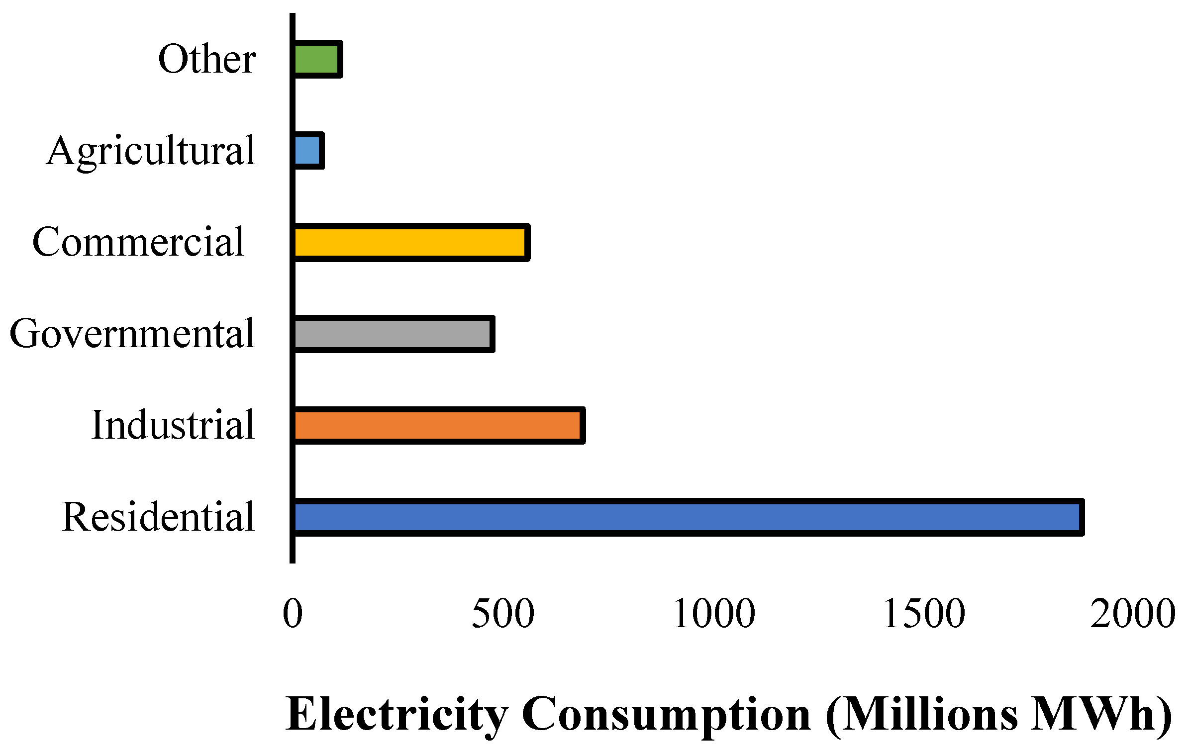
In Saudi Arabia, electricity power generation is regulated by 26 official producers divided into five classes of service providers: Saudi Electricity Company (SEC), Independent Power Producers (IPPs), Jubail and Yanbu Power and Water Utility Company (MARAFIQ), Renewable Energy, Independent Water and Power Producers (IWPPs), and others. The SEC produced around 65% of the total electricity [14]. The total power consumption in Saudi Arabia is split into four provinces, namely eastern, western, central, and southern, and into several sectors, including domestic, agricultural, industrial, commercial, and governmental [14]. Figure 1 shows the comparison of electricity consumption between sectors.
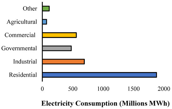
Figure 1.
Total electricity consumption by sectors.
The agricultural sector consumed the lowest amount of electricity, which represents the reality of Saudi Arabia’s agricultural sector [15]. That the agricultural sector had the lowest electricity usage of all the sectors may be due to the dry areas unsuitable for cultivation in several regions of the kingdom. In contrast, the residential sector consumed the largest amount of energy (accounting for 52% of national electricity consumption) of all the sectors, with the industrial sector coming in second, then the commercial, government, and other sectors, respectively. This analytical investigation explains the current growth in urbanization caused by the increasing population and the increment of buildings [16,17]. The demand from the residential sector is predicted to double by 2025 [18,19]. In addition, the residential sector is considerably well comprehended compared to the other sectors. The energy consumption in this sector is mainly expended on light, home appliances, water heating, room cooling, and room heating. Therefore, investigating the electricity consumption in the residential sector and developing forecasting models is an interesting research area.
The electricity demand in Saudi Arabia is rapidly increasing. For example, demand has risen at a 6% yearly pace since 1990 [18]. Moreover, per capita power consumption is fast growing due to urbanization, subsidized fares, and the greater usage of energy-intensive appliances. Thus, the kingdom is eager to deliver the best procedures, plans, and resources for balancing electricity reserve and demand to achieve the optimal balance between electricity generation and consumption [16,20]. Therefore, it is equally essential to forecast the residential electricity consumption and predict total electric energy consumption in Saudi Arabia based on several external features to have a clear and accurate vision of the electricity consumption. However, only a few scholars have been approached to investigate Saudi Arabia’s power demand and consumption [21,22,23]. Most studies in Saudi Arabia focused only on statistical investigation, with a few on electricity consumption forecasting using statistical approaches, including vector auto-regression (VAR), Autoregressive Distributed Lag (ARDL), Electricity Generation Demand for the ith year (EGDi), Regression, ARIMA, SARIMAX, and Harvey’s Structural Time Series [13,21,22,23,24,25,26,27]. Moreover, forecasting energy demand and consumption using machine learning and deep learning has rarely been studied [17].
Consequently, the primary goal of this study is to develop models for forecasting residential electricity consumption (REC) and total electricity consumption (TEC) using a state-of-the-art deep learning method, the LSTM algorithm. In addition, by operating the Bayesian optimization algorithm, this study accelerates automated hyperparameter tuning of the proposed DL models. The Bayesian optimization algorithm is a consecutive design approach for globally optimizing a black box function with no derivatives [6,7]. The following crucial objectives are addressed to achieve the goal of this study:
- (1)
- Investigate the details of the yearly electricity consumption in Saudi Arabia;
- (2)
- Determine the exogenous variables that have a significant impact on REC and TEC;
- (3)
- Apply the long short-term memory algorithm to forecast long-term REC and TEC;
- (4)
- Find the optimum super learner BOA-LSTM model via the Bayesian optimization approach to automatically tune the model’s hyperparameters;
- (5)
- Compare the proposed model to the traditional statistical approaches, namely multiple linear regression and exponential smoothing;
- (6)
- Estimate the performance of the developed models through numerous estimation measures, viz. MAPE, RMSE, MAE, and ;
- (7)
- Forecast and validate forthcoming yearly residential and total electricity consumption.
It is notable that this research specifies employing a super learner BOA-LSTM model for the first time to forecast yearly REC and TEC in Saudi Arabia. The developed long-term electric energy consumption predicting models will enrich the power generation and planning process’s assurance, constancy, and sustainability. The layout of this article is as follows: Section 2 briefly describes the dataset and the proposed models; the results are presented in Section 3; Section 4 presents the relevant discussions; finally, Section 5 states the conclusions, recommendations, and future research plans. Furthermore, to improve the clearness and legibility of this paper, all acronyms have been enumerated at the end of this paper.
2. Materials and Methods
Figure 2 presents the main phases of the methodology used in this study. Firstly, a brief description of the dataset, along with some fundamental statistics, is presented in this section. Then, the mathematical basic and functional fundamentals of the proposed algorithms are explained. The mathematical and theoretical ideas of Bayesian algorithms for tuning the hyperparameters of the LSTM model are also described in this section. Lastly, the performance evaluation measures are demonstrated.
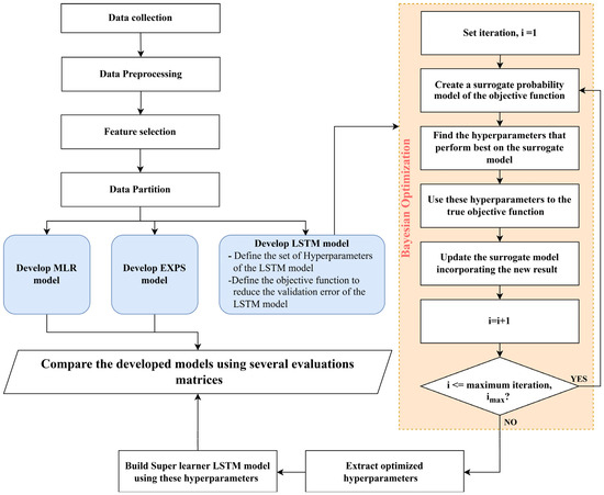
Figure 2.
Methodology used to forecast REC and TEC in Saudi Arabia.
2.1. Data Description
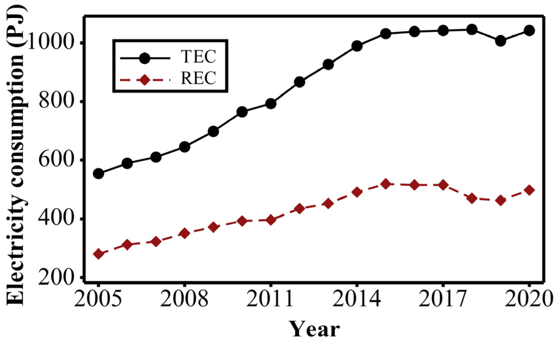
This study used the annual REC and TEC data of the Kingdom of Saudi Arabia from 2005 to 2020. Five exogenous variables were initially considered: GDP, population, production of refined products, imports, and exports. Data sets were collected from the Saudi Central Bank from 2005 to 2020 [14]. Similar increasing trends are observed in yearly TEC and REC time series plots from 2005 to 2020 (see Figure 3).
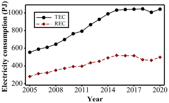
Figure 3.
The general trend of yearly total electricity consumption (TEC) and residential electricity consumption (REC) from 2005 to 2020.
2.2. Computational Techniques
The classical multiple linear regression (MLR), statistical approach exponential smoothing (EXPS), and deep learning algorithm long short-term memory (LSTM) were applied in this research for forecasting yearly residential and total electricity consumption. Model construction and data analysis were performed using SPSS (version 26) and MATLAB (version R2021a).
2.2.1. Multiple Linear Regression (MLR)
MLR is an effective and accurate method for establishing an equation between a dependent variable and several independent variables that serve as predictors [18]. The MLR analysis establishes a mathematical relationship between the input and output values of a linear system, and it identifies which factors have the most binding influence [19,28]. This technique displays the connection between variables. Suppose Y denotes the predicted response/dependent variable and are the independent variables. In that case, the assumption of MLR is that the value of at time is determined by the linear equation Equation (1).
where is the intercept, is known as the coefficient that represents the average change in the response when the variable increases by one unit and all other variables are held constant, and denotes the residual.
2.2.2. Exponential Smoothing (EXPS)
The EXPS is a broadly used statistical method for forecasting time series. The EXPS time series method assigns exponentially decreasing weights for past observations because the weight given to each demand instance decreases exponentially. Simple/single, double, and triple are types of exponential smoothing. Univariate time series data with no trend and no seasonal pattern are forecasted using simple exponential smoothing. This requires a single parameter alpha, called the smoothing factor, that regulates the rate of the effect of earlier observations that will decrease exponentially. The Double exponential smoothing or second-order exponential smoothing, also called Holt’s trend model, is utilized for forecasting time series data with a linear trend but no seasonal pattern. In addition to the smoothing factor alpha parameter, Holt’s trend model requests another smoothing factor called beta that regulates the decline of the effect of variation in trend. In contrast, the triple exponential smoothing algorithm is applied to forecast the time series data with linear trends and seasonal patterns by adding the new smoothing parameter called gamma that regulates the effect of the seasonal factor. This study used double exponential smoothing, Holt’s trend model, to forecast the TEC and REC. The general mathematical formula for Holt’s trend model can be presented as follows [29]:
with the level equation:
and trend equation:
Here, is the forecasted value at future time step , is the most recent observed value of the time series, is the smoothing factor, is the level component, is the trend component, and is the trend-smoothing factor. However, an issue with this current formulation is the assumption that the forecasts will increase or decrease arbitrarily in the future, which is not the reality. Thus, a dampening term, , is frequently added to restrict forecasts of the long term, as follows:
with the level equation:
and trend equation:
2.2.3. Long Short-Term Memory (LSTM)
LSTM models are deep recurrent neural network (RNN) models that have been broadly utilized in various applications such as sentiment and language analysis, voice recognition, and time-series models [30]. An RNN is a form of neural network used to solve sequential problems. It has cyclic connections between many layers, which helps it to memorize the previous knowledge. The output from the deep layers may provide feedback as input to the other layers or the network, along with the next input vector. These recurrent connections work as a memory for the model, allowing it to remember and utilize the order of operations to use as input sequences [30,31]. The typical RNN model has the disadvantage of being difficult to train for problems that require learning long-term temporal correlation. This is due to the vanishing gradient problem, in which the gradient of the loss function decays exponentially with time. The LSTM model was introduced to overcome the vanishing gradient problem [30].
The LSTM model is a complicated RNN network supplemented with memory cells that can store knowledge for long operations [32]. LSTM distinguishes itself from a traditional feedforward neural network in that it has cycles that feed network activations from an earlier time step as inputs to the network to improve predictions at the current time step. As a result of the recurrent connection, the model would create a memory of earlier executions, which is implicitly recorded in its hidden state variables [33]. Therefore, it provides the best results when temporal dependence in sequential data is a significant implicit attribute and learning from earlier phases is required to predict potential trends for the future [31,32,33,34].
The LSTM model comprises three types of gates that govern the flow of information, namely (input, forget, and output). These gates are critical because they determine whether to accept additional inputs, delete the current cell state, or allow the state to influence the output at a specific time step [30,32,34]. The input gate determines what information to add from the current input to the cell state, the forget gate determines what information must be discarded from the cell state, leaving just accurate information, and the output gate determines what information to output from the current cell state. The equations for LSTM are represented as follows [35]:
where stands for the cell state, stands for the hidden state, and represents the logistic sigmoid function that generates numbers between 0 and 1 and describes how much of each component should pass through the gates. The symbol refers to the multiplication that happened during the information flow. In addition, represents the function of the hyperbolic tangent that is used for data bounding purposes, which gives the data range between −1 and 1 to overcome the vanishing gradient problem and generates a new vector that will be added to the cell state [36].
2.2.4. Hyperparameters Optimization for LSTM
The Bayesian optimization algorithm (BOA) was applied in this study since it is an organized process for the global optimization of black box functions. This algorithm is more effective compared to other commonly used optimization procedures such as manual, grid, and random search since they are time-consuming and computationally high-cost [37]. The BOA follows the Bayes’ rule, as shown in Equation (14):
where is a hidden value, is the previous distribution, is the probability, and specifies the posterior distribution. The prior information is used in Bayes’ rule for estimating the posterior possibility, implying that the outcomes of the prior iteration will be used to select values for the next iteration. Consequently, it can achieve the best location faster than random selection [38].
The BOA is divided into two sub-models: substitution and acquisition. The Gaussian process (GP) is a common surrogate for modeling the objective function employed in the replacement model to assess the objective function. GP is a generalization of a Gaussian distribution. After seeing certain function values, GP generally establishes a prior over function that can be transferred into a posterior over function. This process can be described in Equation (15). An additional detailed description of this process can be obtained in [37].
where the function is an understanding of the Gaussian process, is the mean function, and is the covariance function. Here, z is the functional value with any combination in the input domain. The covariance function, also termed a kernel, describes the connection between the variables in the input domains as they are all connected. This kernel is responsible for the smoothness and amplitude of the GP samples. On the other hand, the acquisition function of the Bayesian optimization process depends on previous observations and improves with repetition. The acquisition model suggests the following site to iterate based on the results of the substitution model [38]. The hyperparameter optimization using BOA is mathematically described in Equation (16) as:
where is the objective function to minimalize the validation error, is the set of hyperparameters that yields the minimal value of the objective function, and is any value of space (set of hyperparameters) .
2.2.5. Performance Evaluation Metrics
Properly assessing the model’s accuracy using many statistical measures is crucial because the developed model may perform well with one metric but poorly with another. The following four widely used performance evaluation metrics were calculated to evaluate the created models’ performance using Equations (17)–(20).
where is the number of data points, is the data of the dependent variable, is the data of the exogenous variable, is the standard deviation of data , is the standard deviation of data , is the historical data values, and is the forecasted values.
3. Results
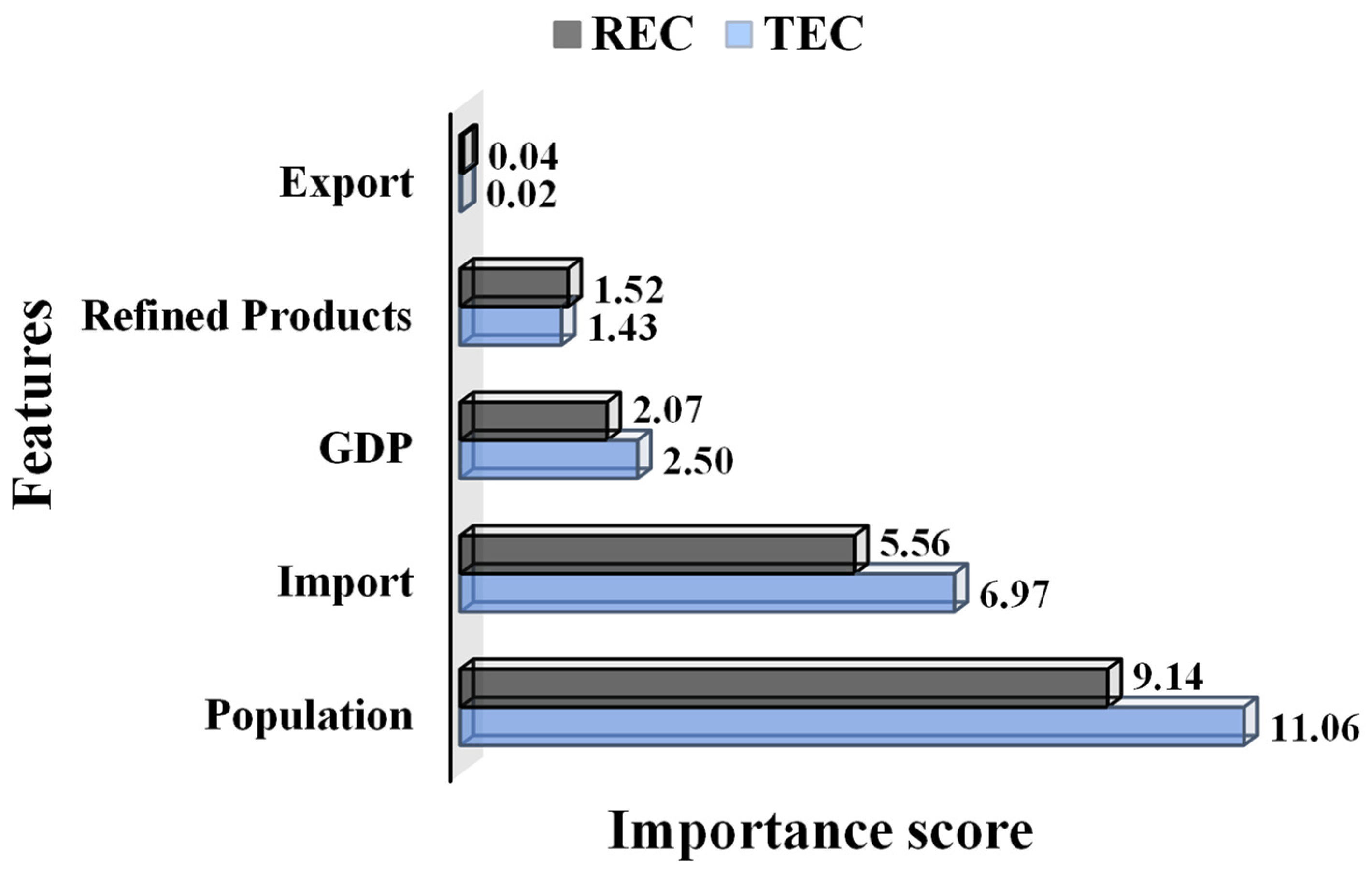
Three statistics and deep learning methods were utilized to develop models for forecasting TEC and REC in Saudi Arabia. Annual data sets for TEC and REC from 2005 to 2017 were used to train the models, and for validation purposes, the data from 2018 to 2020 were used as a validation/test set. As part of data pre-processing, data were standardized. There are five features in the original datasets. However, this feature set may contain redundant data that can increase computing costs and affect predicting accuracy. Thus, various feature selection algorithms, including the Pearson correlation coefficient, F-tests, sequential feature selection, neighborhood component analysis, and rank importance of predictors using the RReliefF algorithm, were used for selecting the most significant features of REC and TEC. Based on the correlation coefficient analysis results shown in Table 1 and Table 2, the descriptive features that have a substantial association with REC and TEC are GDP, population, imports, and refined products, since the p-values for all these variables are very small. In contrast, the variable export is insignificant since both p-values are greater than 0.5. Other feature selection algorithms’ results also show that export is insignificant. Figure 4 depicts the overall rating of the attributes. Thus, the four exogenous variables used to apply forecasting models are GDP, population, imports, and refined products.

Table 1.
Results of the correlation analysis between REC and the studied features.
Table 2.
Results of the correlation analysis between TEC and the studied features.
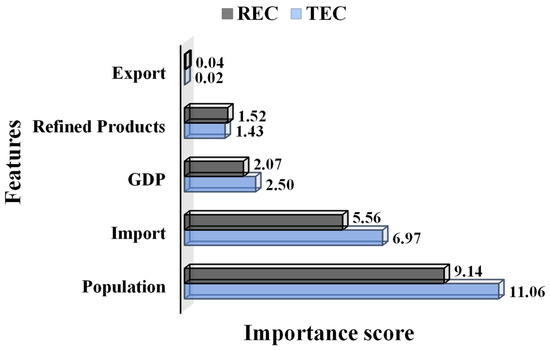
Figure 4.
Features ranking for TEC and REC.
3.1. Development of Forecasting Models
This study developed three models, viz. MLR, EXPS, and LSTM, for forecasting yearly residential and total electricity consumption.
3.1.1. Development of MLR Model for TEC and REC
Table 3 presents the model summary of the developed MLR models for TEC and REC. As shown in the models’ summary, in the MLR model for REC, all the features are significant at a 5% significance level, and the most significant feature is imports. In the MLR model for TEC, GDP is not substantial, and the population is the most important factor. The AIC (Akaike information criterion) for the MLR (TEC) model is 161.4221, while the AIC for the MLR (REC) model is 143.2073. The performance, based on several performance measures, including MAE, RMSE, and MAPE, for the training and testing datasets is presented in Table 4. As demonstrated in Table 4, no significant changes in training and testing dataset performance were detected in either the MLR (TEC) or MLR (REC) models, showing that the created models are neither underfitted nor overfitted.
Table 3.
Model summary of the developed MLR models.
Table 4.
Forecasting performance of the developed models based on the training (from 2005 to 2017) and testing (from 2018 to 2020) datasets.
3.1.2. Development of EXPS Model for TEC and REC
Holt’s linear trend exponential smoothing algorithm was applied in this study to develop forecasting models for both TEC and REC. This algorithm highly depends on the value of three hyperparameters, namely smoothing factor alpha, trend smoothing factor beta, and dampening term . Table 5 presents the values of these hyperparameters of the developed model. The AIC for the EXPS(TEC) model is 108.554, while the AIC for the EXPS(REC) model is 103.704. Similar performance for training and testing data was observed for the developed EXPS(TEC) and EXPS(REC) models; thus, the models are neither underfitted nor overfitted (see Table 4).
Table 5.
Hyperparameters and model summary of the developed Holt’s trend exponential smoothing model.
3.1.3. Development of LSTM Model for REC and TEC
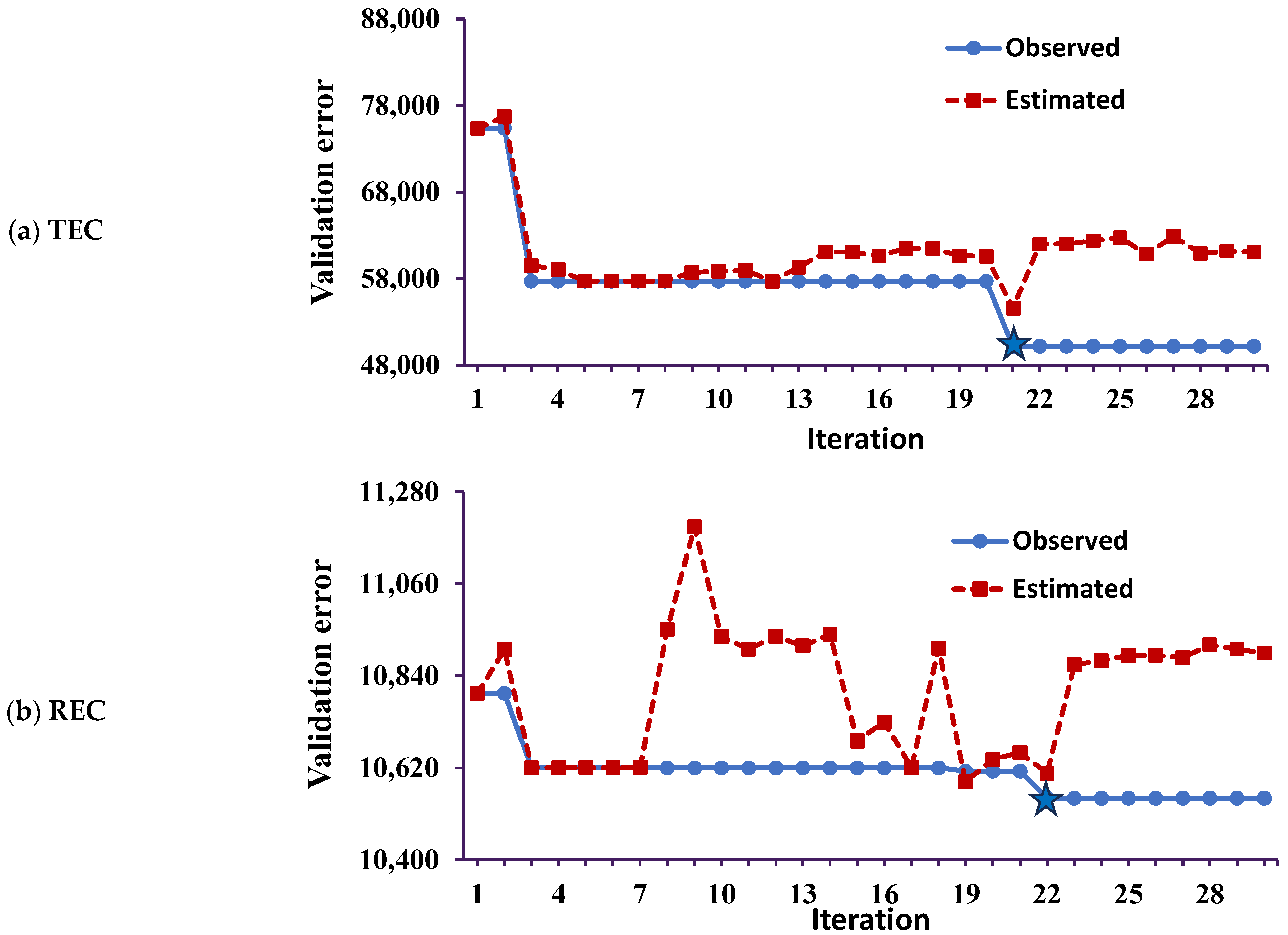
The performance of the LSTM model depends significantly on hyperparameters (viz. number of LSTM layers, number of units in each layer, initial learning rate, L2Regularization, the maximum number of epochs, and minibatch size) [22]. The BOA approach was applied along with several experiments to attain the optimal values of the hyperparameters. The progress of the hyperparameter optimization and the feasible operating point is shown in Figure 5. The best possible point is where the observed objective validation error is the least. The minimum observed objective validation error (50,170.46) for the LSTM(TEC) model was obtained at the 21st iteration, and the minimum score (10,547.34) for LSTM(REC) was found at the 22nd iteration. The tuned hyperparameters were achieved at these locations, and the tuned hyperparameters used to determine the optimal super learner BOA-LSTM models for TEC and REC are presented in Table 6.

Figure 5.
The progress of BOA in tuning hyperparameters of LSTM model: (a) TEC and (b) REC. The estimated validation error is the result of the surrogate probability model, while the observed validation error is the value of the true objective function. The best feasible point ★ 50,170.46 was observed for LSTM(TEC)at iteration 21 (a), and 10,547.34 for LSTM(REC) at iteration 22.
Table 6.
Optimized LSTM hyperparameters obtained using BOA along with several experiments.
The total computational elapsed time was not too high (742.38 s for BOA-LSTM(TEC) and 392.46 s for BOA-LSTM(REC)). However, developing any super learner model for a specific dataset entails significant time, research, and computational trials (experiments). Thus, obtaining an optimized model is necessary, and BOA performs a crucial role. Recently, deep learning methods have become one of the essential research areas across various engineering branches, including its application under the attention of energy research. Hence, such a super learner-based modeling approach is a state-of-the-art application and a potential research area.
3.2. Performance Evaluation and Model Comparison
A forecasting model’s prediction accuracy, generalizability, and computational efficiency are crucial characteristics; thus, these characteristics of the established models were compared in this study.
3.2.1. Prediction Accuracy of the Developed Models
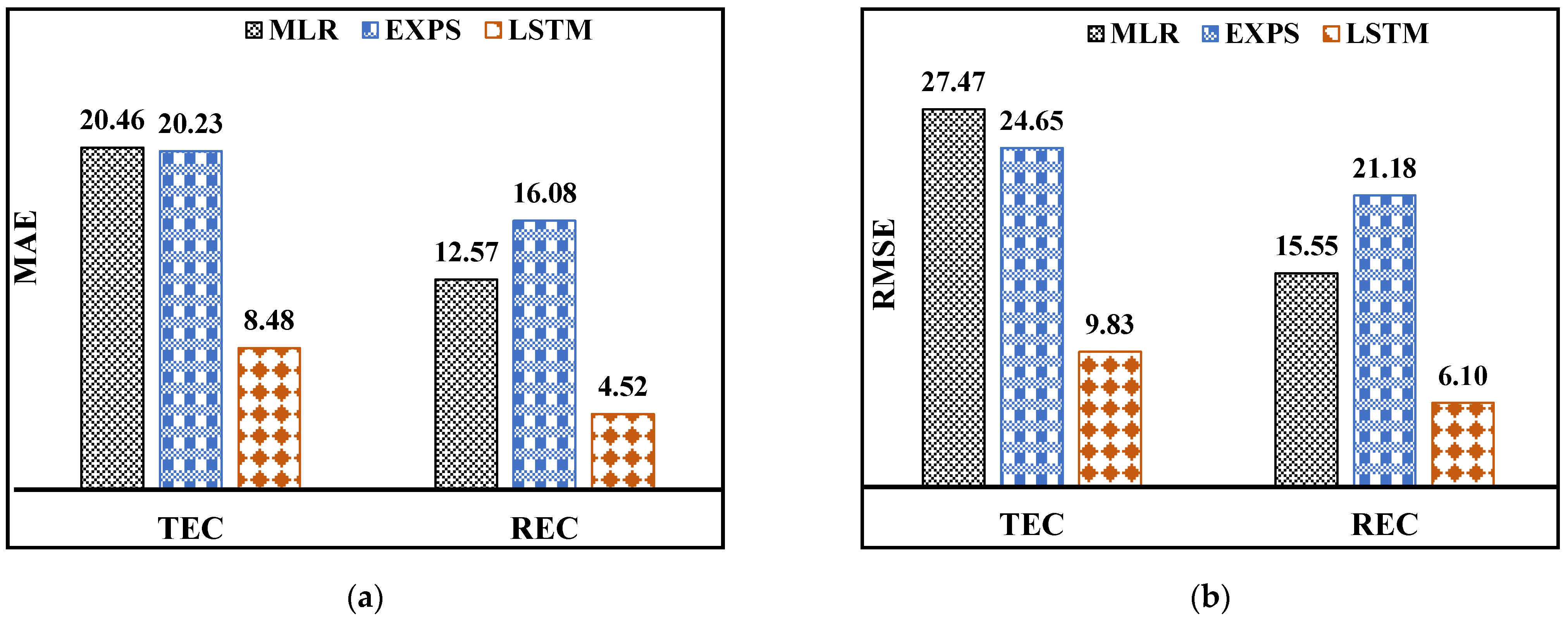
The overall model performance was assessed based on various performance indicators for the total historical data from 2005 to 2020 (see Figure 6). Outstanding forecasting performance was observed in all the developed models ( for TEC and for REC). However, the LSTM model developed for both TEC and REC performed the best (MAPE and of LSTM(TEC) are 1.05, and 0.998, respectively; MAPE and of LSTM(REC) are 1.13, and 0.988, respectively). EXPS(TEC) performed better than MLR(TEC), while the developed MLR(REC) performed better than EXPS(REC). The performance improvements of the developed LSTM models compared to the MLR and EXPS models for both TEC and REC are presented in Table 7. A performance improvement of 58.2% in MAE and 64.2% in RSME was provided by the BOA–LSTM(TEC) model compared to the MLR(TEC), while it is 58.1% in MAE and 60.1% in RMSE to the EXPS(TEC) model. However, a performance improvement of 64.0% in MAE and 60.8% in RMSE was provided by the BOA–LSTM(REC) model compared to the MLR(REC) model, while it is 71.9% in MAE and 71.2% in RMSE compared to the EXPS(REC) model. Thus, the overall results indicate that the BOA–NLSTM predictions agree well with the historical data.
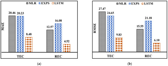
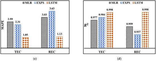
Figure 6.
Performance comparison of the developed BOA-LSTM model with the MLR and exponential smoothing model: (a) MAE, (b) RMSE, (c) MAPE, and (d) .
Table 7.
Performance improvement of the developed BOA-LSTM models compared to the MLR and EXPS models for TEC and REC.
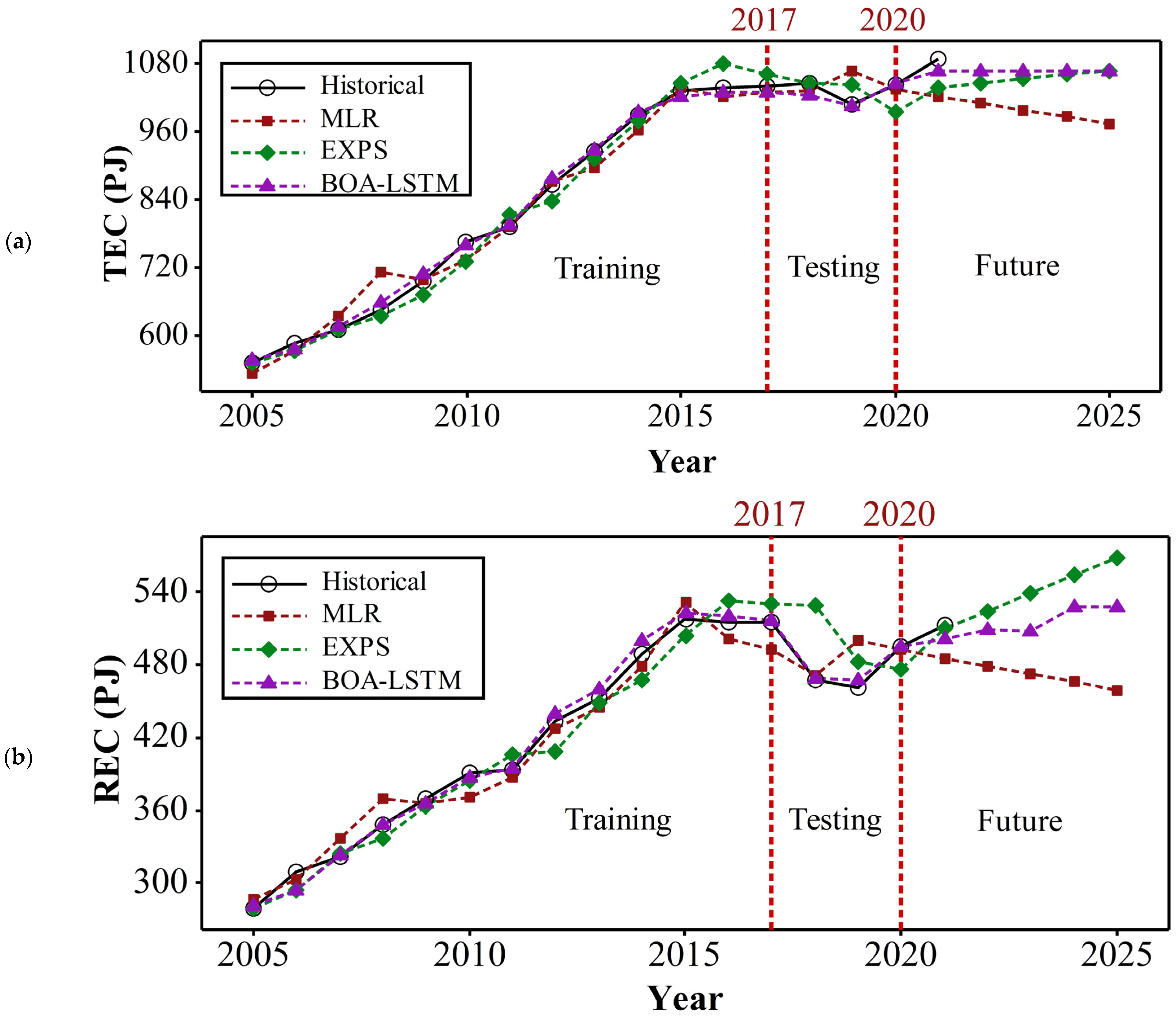
Figure 7 compares historical TEC and REC with the forecasted values for training, testing, and the next five years based on the developed MLR, EXPS, and BOA-LSTM models. The outstanding ability to achieve the TEC forecasts was observed in all developed models. However, the EXPS shows poor estimates in the testing period, while the forecasted values of the other two models nearly overlay with the historical data.
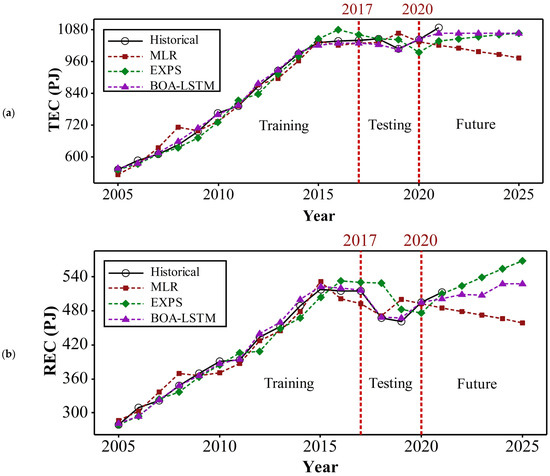
Figure 7.
Comparison between the historical data with forecasted (a) TEC and (b) REC of the three proposed models for training, testing, and next five years.
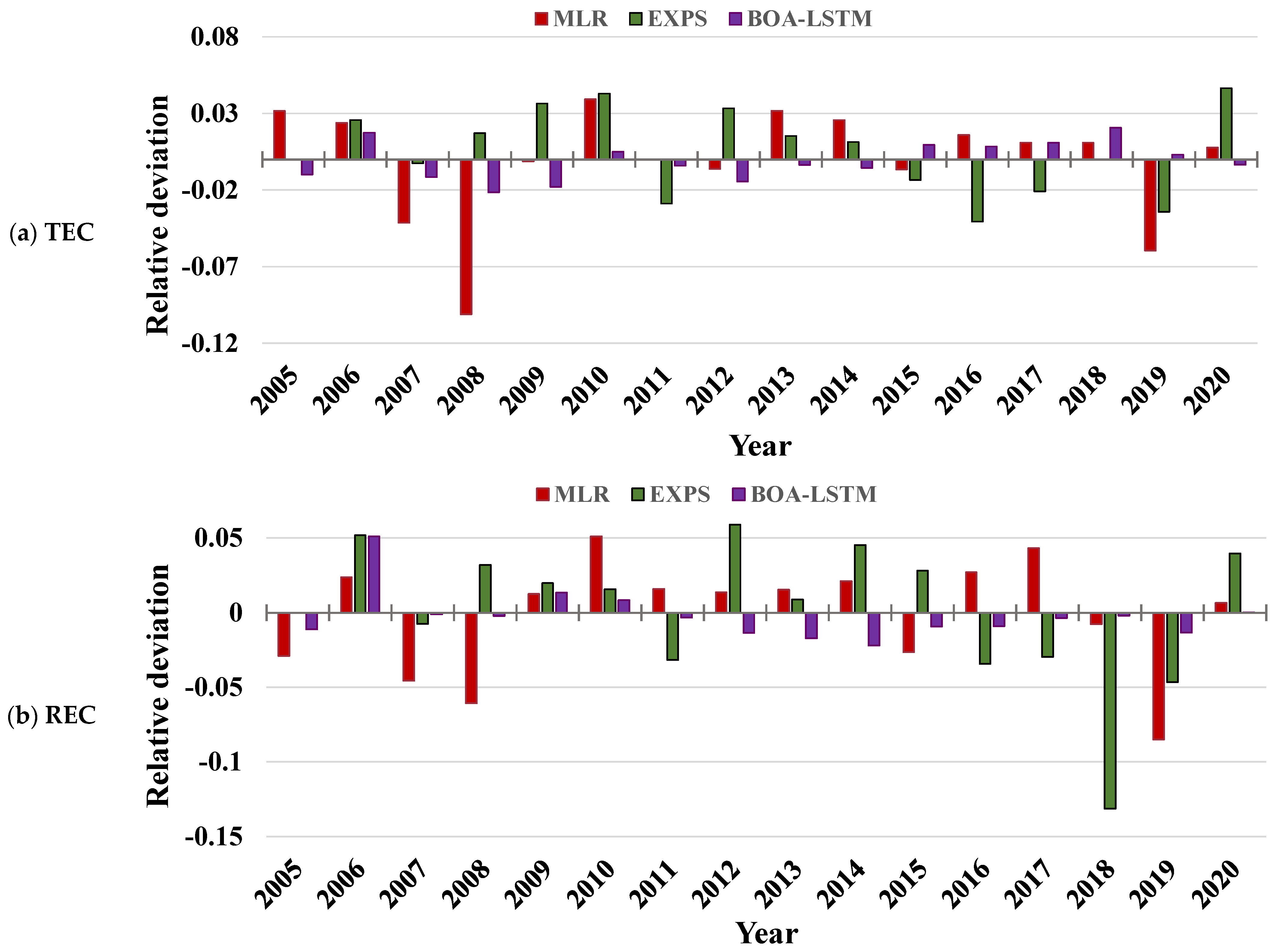
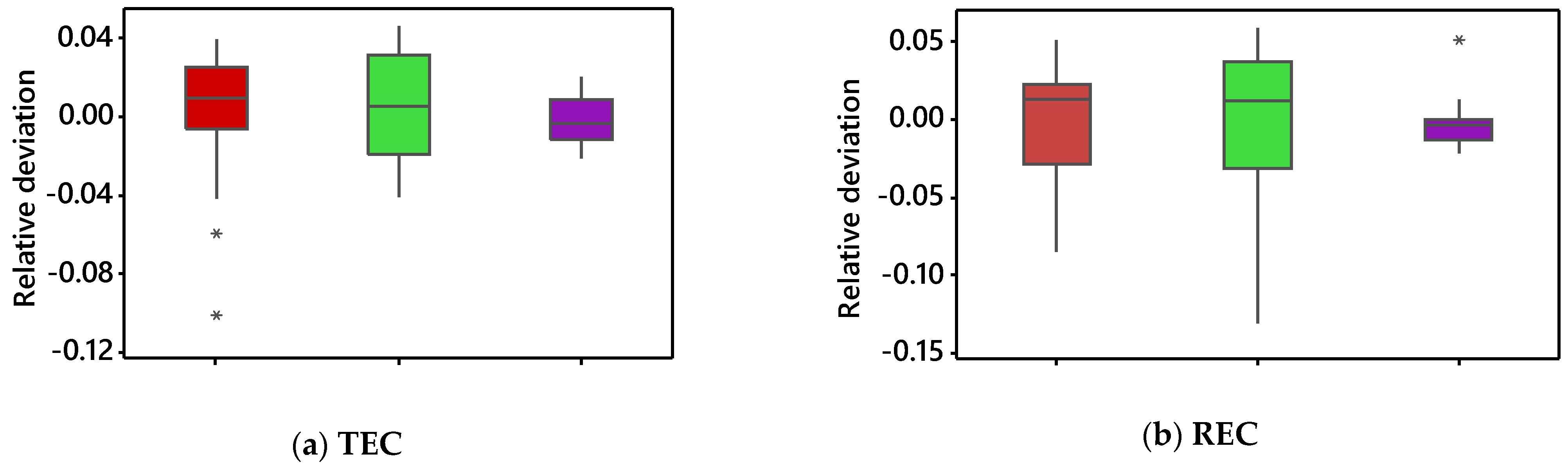
A yearly indexed error analysis for the whole dataset was conducted to analyze how the BOA-LSTM models improve year-ahead electricity consumption predictions compared to the MLR and EXPS models. The relative deviations of the predicted REC and TEC for all the developed models from the historical data are presented in Figure 8. Relative deviations in most years for all models are scattered around the zero line, indicating the high forecasting capability of the developed models. However, a comparatively high relative deviation for TEC forecasting by MLR was observed in 2008 and 2019, while the highest variation for REC forecasting by the EXPS model in 2018 was observed. For further evaluation, the range of the relative deviations in the yearly forecasting TEC and REC were analyzed based on the boxplot (Figure 9). It can clearly be observed that the BOA-LSTM has a lower range of relative deviation from the historical data than the MLR and EXPS models for both the TEC and REC.
Figure 8.
Relative errors of every year for the total dataset based on the three developed models for (a) TEC and (b) REC.
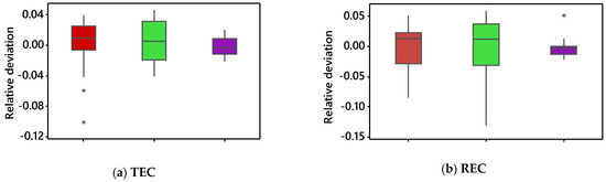
Figure 9.
Box plots of relative deviation in the yearly forecasted (a) TEC and (b) REC based on the developed models. Here * represents the outlier.
3.2.2. Generalizability of the Developed Models
The study calculated the forecasted values for the next five years (2021–2025) using the features produced by the SPSS to investigate the generalizability of the developed model. The future predicted values of the TEC and REC are presented in Figure 7. The future forecasting for the EXPS and BOA-LSTM models has a similar trend, and the forecasted values are very close to each other, especially in TEC forecasting, suggesting that the developed EXPS and BOA-LSTM models are comparable. The future forecasting capability of the developed models was further analyzed by comparing the forecasted TEC and REC in 2021 with the latest updated data released in 2021 [39], and the results are shown in Table 8. The results indicate a good forecasting ability for all the developed models, while outstanding performance was observed in the BOA-LSTM model for both TEC and REC, and the lowest error in REC was found in the EXPS model.
Table 8.
Performance comparison between the original data and the three forecasting models.
4. Discussion
Long-term electricity consumption forecasting is vital in electric power system management, price regulation, and energy transactions. Several studies were conducted around the globe on electricity consumption forecasting because of its significant role in electric power management, especially in supporting policymakers to develop strategies for ensuring energy sustainability. Various artificial intelligence approaches were used for forecasting long-term electricity consumption [1,2,3,4,5,6,7,8,9,10,40,41].
Numerous studies were conducted to analyze electric energy consumption using various classical statistical approaches. The association between the gross domestic product and the electricity consumption peak load in Saudi Arabia was investigated by Alsaedi et al. in [22]. A vector auto-regression (VAR) analysis linked with some tests, viz. the forecast error variance decompositions, the impulse response function, and Granger causality testing, was used in this study. The results of this study demonstrate a growth rate for electricity consumption, pick load, and GDP of 7.21%, 6.87%, and 14.14%, respectively, higher in the past ten years. Saudi Arabia’s power demand per capita was compared to that of the UAE and Australia by Ouda et al. [21]. The authors claimed that Saudi Arabia consumed the least power compared to UAE and Australia. The electric energy usage from 2014 to 2040 was also forecasted in this study by computing the Electricity Generation Demand () for the year in million GW.
The Autoregressive Distributed Lag (ARDL) cointegration technique and Augmented Dickey–Fuller (ADF) test were applied to determine the connection of electricity use with the financial market development in Saudi Arabia by Senan et al. [23]. Based on the outcomes of this research, electricity consumption is positively associated with urbanization and economic development, thus positively affecting financial market development. The impact of social distancing during the COVID-19 pandemic on electric energy use and temperature in Saudi Arabia was investigated by Alkhraijah et al. in [24]. An outline of the impact of social distance and energy usage in several countries was presented in this research. Then, as a case study, the impact of social distancing policies in Saudi Arabia was explored. The relationship between daily temperature and average power consumption was examined by applying the linear correlation coefficient. Furthermore, this association during the curfew period (from 6 to 26 April 2019) was extensively investigated and compared to the past five years. A noteworthy relationship was observed between electricity usage and temperature: high electricity demand when the temperature is high, mainly for cooling during the curfew.
A Structural Time Series algorithm was applied to investigate the impact of weather conditions, energy prices, and income on the electricity consumption of residential buildings by Mikayilov et al. in [25]. The energy cost changed through the western, eastern, southern, and central regions, varying from 0.20 in the central area to 0.46 in the eastern area. Likewise, a diverse effect of income was observed, fluctuating from 1.02 in the western part to 0.27 in the eastern part. Lastly, hot weather is strongly associated with electricity consumption in all provinces. In addition, Alarenan et al. [26] utilized the Structural Time Series Model (STSM) algorithm to develop a model that accumulated the industrial energy demand and some economic development factors in Saudi Arabia. Based on the outcomes of this study, the total demand for industrial energy is influenced by energy prices and incomes. Thus, industrial energy demand will increase continuously in the forthcoming years, in response to economic development. Raising energy prices could increase the chance of decreasing this growth. Nevertheless, in 2016, Saudi Arabia suggested an agenda that opposed increasing the expenses of some facilities like electricity, water, and fuel for residential and industrial sectors. Increasing these prices caused a substantial drop in consumption by 6.9%, around 3.0 million tons.
Some studies considered temperature as a substantial factor that influences electricity consumption. An econometric model was developed by AL-Zayer et al. in [27] to forecast electricity consumption based on the consequence of the nearby weather temperature in the eastern province of Saudi Arabia. This study used regression analysis for each year (from May to September) separately to assess the effect of temperature on electricity consumption. Five years’ worth of historical data were then applied to forecast the demand for electric energy. Based on the results of this study, the proposed models that attained the best performance for predicting electricity consumption were linear and quadratic at the 5% level assessed by MAPD, MSPE, and . Moreover, the cyclical sinusoidal autoregressive model was developed for forecasting electricity consumption for twelve months, separated into two equal parts. The regression model performed better than the quadratic and sinusoidal models. In addition, a regression model was developed to forecast EC using monthly data from August 1987 to July 1992 in Saudi Arabia [42]. Several significant features (population, temperature, humidity, and solar radiation) were considered via the stepping-regression approaches. The selected features are significantly associated with electricity consumption; predominantly, the weather temperature significantly impacts the demand stability. The authors proposed that the stated model be employed to estimate future electricity consumption.
A computable general equilibrium model (CGE) was developed by Soummane et al. in [43] to estimate sectoral electricity demand in Saudi Arabia until 2030. The study expected total Saudi power demand to expand much slower over the next decade than previous trends. This study claimed that according to the baseline assumption, this demand will reach 365.4 (TWh) by 2030. However, the electricity demand in the industrial and services sectors is expected to expand faster than in the residential sector. The authors suggested that enforcing efficiency rules can cut overall power demand by up to 118.7 TWh, and successfully implementing the suggested strategies may result in considerable energy savings. Aldubyan et al. in [44] illustrated that Saudi homes increased their energy consumption throughout the COVID lockdown period. The hourly electricity consumption and weather data from 15 March to 15 June 2020 were used in this study. The authors presented a validated Residential Energy Model (REEM) that predicted a 25.2% increase in overall power usage in Saudi houses. An updated assessment predicted that, when adjusted for meteorological conditions, the 2020 stay-at-home directive resulted in a 16.0% increase in house energy usage owing to increased lights and appliances such as air conditioning being used to survive the hot temperatures. Furthermore, the researchers focused on the transition to working from home, and the findings show that Saudi housing stock energy consumption will rise by 13.5% because of long-term stay-at-home living.
Several studies applied a widely used statistical approach, viz. ARIMA, to develop a long-term forecasting model [7,13,45,46,47]. The electric energy consumption in the Eastern province of Saudi Arabia was predicted based on features related to meteorological, demographic, and economic statistics by Abdel-aal et al. in [46]. The ARIMA model was developed using monthly data from August 1987 to July 1993. The performance of the developed ARIMA model was compared with other models, namely the Abductory Induction Mechanism (AIM) and multivariate regression models. With mean percentage errors of 3.8%, the ARIMA model achieved better performance in forecasting EC compared to the multivariate regression (5.6%) and AIM (8.1%). Fahmy et al. [47] developed models to forecast the electric energy consumption in Saudi Arabia using two algorithms, polynomial and ARIMA, based on the data from 1990 to 2019. The results of this study demonstrate that the polynomials model has the advantage of being capable of representing a broad range of mathematical models.
In [13], Alharbi et al. developed long-term SARIMA models to forecast several electric sectors, including electric energy generation, consumption, installed capacity, and peak load. The yearly data from 1980 to 2020 in Saudi Arabia were used in this research. All the proposed models have promising performance ( = 0.99 and MAPE ≤ 0.40). However, this study did not include any exogenous variable, and the authors recommended that investigating additional exogenous features and their associations may enhance the research and forecasting accuracy. The Prophet model’s effectiveness in long-term peak load forecasting in Kuwait was first examined by Almazrouee et al. in [36]. The Prophet model was compared with exponential smoothing models to examine forecasting long-term peak loads. The developed Prophet model performed best based on the five evaluation measures.
Recently, machine-learning- and deep-learning-based approaches have been widely used in energy research. Sharma et al. [45] described time series-based methods, namely, SARIMA, exponential smoothing, random forest, and LSTM, for predicting medium-term energy load in the agricultural sector in India. The developed SARIMA and exponential smoothing models performed better than the LSTM and random forest models. However, the exponential smoothing model performed the best, with the lowest RMSPE= 7.98%. Cho et al., in [7], developed hybrid models SARIMAX-ANN, SARIMAX-SVR, and SARIMAX-LSTM for forecasting peak load in Korea. The hybrid models performed considerably better than the SARIMAX model. However, the hybrid SARIMAX-LSTM model performed the best, with the lowest MAPE of 3.4737 and the highest value of . Khalid et al. [10] established a JLSTM model to estimate the electricity load and price using data from diverse big data resources. The hourly data were used to develop the suggested models for predicting electricity demand and price for a week, a month, and three months. The suggested models were evaluated with other models based on univariate LSTM and SVM. Based on the results of this study, the proposed model performed the best.
A long short-term memory autoencoder (LSTM-AE) model was developed using an hourly dataset from American Electric Power from 2004 to 2018 by Saoud et al. [48]. The Particle Swarm Optimization (PSO) algorithm was applied in this study to find the optimum hyperparameters of the LSTM model. The performance of the proposed model was compared with other AI-based models: LSTM, CNN, ANN, and random forest. The best performance was observed in the proposed model with RMSE = 680.89 and MAE = 486.28. In [49], Peng et al. used LSTM-based models to forecast energy consumption using monthly data in China. This study considered external variables: Industrial Sales Value, Industrial Sales Ratios, Export Delivery Value, Industrial Fixed assets investment Value, Export, Import, and Producer Price Index. The proposed (Empirical Wavelet Transform) EWT-attention-LSTM prediction model outperformed specific current energy consumption prediction models.
Hadjout et al. in [50] forecast monthly power consumption for the Algerian economic sector utilizing monthly data from 2006 to 2019. Three deep learning models, viz. LSTM, Gated Recurrent Unit (GRU), and Temporal Convolutional Networks (TCN), were developed in this study. The grid search algorithm was used to find the optimal weight coefficients of each model. The developed TCN model achieved the minimum RMSE compared to other models. The LSTM model was developed by Alraddadi et al. in [41] to optimize electricity consumption in London homes. The dataset in this article is divided into daily and monthly usage to compare current network topologies in previous studies. Compared to various network topologies, the suggested model had the highest accuracy, with an RMSE of 0.362 and an MAE of 17.8%.
A comparative summary of the related research is presented in Table 9. It can be noted that a minimal study focuses on developing models to forecast long-term electricity consumption in Saudi Arabia. Moreover, few studies applied machine-learning and deep-learning algorithms to establish EC forecasting models. Most research did not incorporate exogenous variables, particularly population, GDP, refined oil products, imports, and exports. However, these variables may substantially affect EC forecasting, especially in Saudi Arabia. Few scholars employed automated optimization methods to properly adjust the hyperparameters of ML models. It is noteworthy that optimized hyperparameters extensively influence the model’s predicted performance. In addition, none of these researchers applied BOA to tune the optimized hyperparameters systematically. As mentioned in the very last row of Table 9, the novelty of this study lies in the fact that this is the first paper that developed separate long-term forecast models for TEC and REC in Saudi Arabia using a deep learning-based algorithm, namely LSTM; it includes several significant exogenous variables (population, GDP, refined oil products, and imports) to develop forecasting models; it applied BOA for tune-optimized hyperparameters; and it developed novel super learner models BOA-LSTM(TEC) and BOA-LSTM(REC) for forecasting TEC and REC, benchmarked with the classical statistical method MLR and time series method EXPS depending on a range of metrics, including generalizability and time complexity.
Table 9.
Comparative table of reported studies.
Studies on forecasting electric energy consumption are still at the developing or lacking stage in Saudi Arabia. Thus, this research could significantly contribute to Saudi Arabia’s development by offering an upcoming assessment of long-term electricity consumption to guarantee the sustainability of electric energy. The benefit of using the proposed research can be noticed in Figure 6 and Table 7. All the developed models had a low error (MAPE < 3.64%) and a high coefficient of determination (%), indicating outstanding forecast capacities. On the other hand, the hybrid BOA-LSTM models have the best prediction performance (MAPE around 1% and for both TEC and REC). The satisfactory results in this study were achieved based on the optimal application of the feature selection methods, hyperparameter optimization algorithm BOA, and the state-of-the-art deep learning algorithm LSTM.
5. Conclusions
The Kingdom of Saudi Arabia has recently become one of the leading nations in sustainable energy. In this regard, the kingdom is aiming to adopt cutting-edge technology and solutions that catalyze optimal energy utilization. Saudi Arabia has made significant progress in various areas, including education, medicine, engineering, urban development, and particularly in the economic and industrial sectors, which need immense amounts of several kinds of energy, including electrical, fuel, and solar. In addition, electricity is the most extensively utilized energy in all domains, including factories, hospitals, schools, industrial fields, and residential properties. The Saudi Electricity Company is primarily responsible for supplying electricity nationwide. Because of the elevated electric energy consumption, the electricity company must investigate and evaluate the current demand and all variables influencing the growth or reduction in electricity consumption to sustain services. The digital transmission of all sectors is likewise essential to make data accessible for research to enhance planning goals for future development.
The residential and total electric energy consumption in Saudia Arabia was studied in this research. After applying multiple feature selection algorithms, population, GDP, imports, and refined oil products were considered the exogenous variables of electric energy consumption. A state-of-art deep learning algorithm, viz. LSTM, was applied to forecast yearly REC and TEC and compared with MLR and EXPS models for validation. In addition, the hybrid BOA-LSTM model was developed using the Bayesian optimization algorithm for tuning the model’s hyperparameters automatically and efficiently. The developed models’ performances were estimated through several performance measures. A low prediction error (MAPE < 3.64%) and a high coefficient of determination (%) was observed in all the developed models, signifying outstanding forecast capabilities. Moreover, the super learner BOA-LSTM models have the best prediction capabilities (MAPE around 1% and for both TEC and REC). Correspondingly, this study will boost Saudi Arabia’s advancement by offering a long-term picture of power usage to ensure electric energy’s sustainability. Additionally, feasibility studies on solar and wind energy are insufficient to support the deployment of renewable energy sources and the divergence of energy fusion. The researchers intend to build and improve deep learning models to forecast wind speed and sun radiation in various places using historical data.
Author Contributions
S.H.A.: resources, data collection, software, methodology, visualization, and writing; N.S.: conceptualization, software, methodology, visualization, writing—review and editing. All authors have read and agreed to the published version of the manuscript.
Funding
This research received no external funding.
Data Availability Statement
Datasets are available from the corresponding author upon reasonable request.
Acknowledgments
All authors would like to acknowledge Imam Abdulrahman Bin Faisal University for supporting this research and other facilities. We thank the anonymous reviewers for carefully reading our manuscript and for many insightful comments and suggestions.
Conflicts of Interest
The authors declare no conflict of interest.
Abbreviations
The following abbreviations are used in this manuscript:
| Abbreviation | Description | Abbreviation | Description |
| ACF | Autocorrelation Function | KWh | Kilowatt hour |
| ADF | Augmented Dickey Fuller | LEAP | Long-range Energy Alternative Planning |
| AIM | Abductory Induction Mechanism | LSTM | long short-term memory |
| ANN | Artificial Neural Network | MA | Moving Average |
| AR | Auto-Regressive | MAE | Mean Absolute Error |
| ARDL | Autoregressive Distributed Lag | MAPD | Mean Absolute Percentage Deviation |
| ARIMA | Autoregressive Integrated Moving Average | MAPE | Mean Absolute Percentage Error |
| ARIMAX | Autoregressive Integrated Moving Average with Exogenous Inputs | MARAFIQ | Power and Water Utility Company for Jubail and Yanbu |
| BOA | Bayesian Optimization Algorithm | ML | Machine Learning |
| CGE | Computable General Equilibrium | MLR | Multiple Linear Regression |
| CNN | Convolutional Neural Network | MSPE | Mean Square Percentage Error |
| CVRMSE | Coefficient of the Variation in the Root Mean Square Error | MW | Megawatt |
| DE | Differential Evolution | PACF | Partial Autocorrelation Function |
| DL | Deep-Learning | PJ | Petajoule |
| EC | Electricity Consumption | PSO | Practical Swarm Optimization |
| ECON | Economic Factor | RE | Relative Error |
| EGDi | Electricity Generation Demand for i | REC | Residential Electricity Consumption |
| EL | Electric Load | REEM | Residential Energy Model |
| ENVI | Environmental Factor | RF | Random Forest |
| EP | Electric Price | RMSE | Root Mean Square Error |
| EXPS | Exponential Smoothing | RNN | Recurrent Neural Network |
| EXT | Empirical Wavelet Transform | SA | Simulated Annealing |
| GA | Genetic Algorithm | SEC | Saudi Electricity Company |
| GDP | Gross Domestic Product | SEM-VARIMAX | Structural Equation Modelling-Vector Autoregressive with Exogeneous Variables |
| GP | The Gaussian process | SOCI | Social Component |
| GRU | Gated Recurrent Unit | STSM | Structural Time Series Model |
| GW | Gigawatt | SVR | Support Vector Regression |
| ICA | Independent Component Analysis | TCN | Temporal Convolutional Networks |
| IPPs | Independent Power Producers | TEC | Total Electricity Consumption |
| IQR | Inter Quartile Range | TMY | Typical Meteorological Year |
| IWPPs | Independent Water and Power Producers | TWh | Terawatt hour |
| JLSTM | Jaya Long Short-Term Memory | UAE | United Arab Emirates |
| KPX | Korea Power Exchange | VAR | Vector Auto-Regression |
| KSA | Kingdom of Saudi Arabia | The Coefficient of Determination |
References
- Khan, A.; Chiroma, H.; Imran, M.; Khan, A.; Bangash, J.I.; Asim, M.; Hamza, M.F.; Aljuaid, H. Forecasting Electricity Consumption Based on Machine Learning to Improve Performance: A Case Study for the Organization of Petroleum Exporting Countries (OPEC). Comput. Electr. Eng. 2020, 86, 106737. [Google Scholar] [CrossRef]
- Kaboli, S.H.A.; Selvaraj, J.; Rahim, N.A. Long-Term Electric Energy Consumption Forecasting via Artificial Cooperative Search Algorithm. Energy 2016, 115, 857–871. [Google Scholar] [CrossRef]
- Ur Rehman, S.A.; Cai, Y.; Fazal, R.; Das Walasai, G.; Mirjat, N.H. An Integrated Modeling Approach for Forecasting Long-Term Energy Demand in Pakistan. Energies 2017, 10, 1868. [Google Scholar] [CrossRef]
- Kankal, M.; Uzlu, E. Neural Network Approach with Teaching–Learning-Based Optimization for Modeling and Forecasting Long-Term Electric Energy Demand in Turkey. Neural Comput. Appl. 2017, 28, 737–747. [Google Scholar] [CrossRef]
- Yukseltan, E.; Yucekaya, A.; Bilge, A.H. Hourly Electricity Demand Forecasting Using Fourier Analysis with Feedback. Energy Strategy Rev. 2020, 31, 100524. [Google Scholar] [CrossRef]
- Snoek, J.; Larochelle, H.; Adams, R.P. Practical Bayesian Optimization of Machine Learning Algorithms. Adv. Neural Inf. Process. Syst. 2012, 25, 2960–2968. [Google Scholar]
- Lee, J.; Cho, Y. National-Scale Electricity Peak Load Forecasting: Traditional, Machine Learning, or Hybrid Model? Energy 2022, 239, 122366. [Google Scholar] [CrossRef]
- Sutthichaimethee, P.; Naluang, S. The Efficiency of the Sustainable Development Policy for Energy Consumption under Environmental Law in Thailand: Adapting the SEM-Varimax Model. Energies 2019, 12, 3092. [Google Scholar] [CrossRef]
- Aurangzeb, K.; Alhussein, M.; Javaid, K.; Haider, S.I. A Pyramid-CNN Based Deep Learning Model for Power Load Forecasting of Similar-Profile Energy Customers Based on Clustering. IEEE Access 2021, 9, 14992–15003. [Google Scholar] [CrossRef]
- Khalid, R.; Javaid, N.; Al-zahrani, F.A.; Aurangzeb, K.; Qazi, E.U.H.; Ashfaq, T. Electricity Load and Price Forecasting Using Jaya-Long Short Term Memory (JLSTM) in Smart Grids. Entropy 2020, 22, 10. [Google Scholar] [CrossRef]
- Aasim; Singh, S.N.; Mohapatra, A. Data Driven Day-Ahead Electrical Load Forecasting through Repeated Wavelet Transform Assisted SVM Model. Appl. Soft Comput. 2021, 111, 107730. [Google Scholar] [CrossRef]
- Haq, M.R.; Ni, Z. A New Hybrid Model for Short-Term Electricity Load Forecasting. IEEE Access 2019, 7, 125413–125423. [Google Scholar] [CrossRef]
- Alharbi, F.R.; Csala, D. A Seasonal Autoregressive Integrated Moving Average with Exogenous Factors (SARIMAX) Forecasting Model-Based Time Series Approach. Inventions 2022, 7, 94. [Google Scholar] [CrossRef]
- Yearly Statistics. Available online: https://www.sama.gov.sa/en-us/EconomicReports/pages/YearlyStatistics.aspx (accessed on 3 May 2022).
- Krarti, M.; Aldubyan, M.; Williams, E. Residential Building Stock Model for Evaluating Energy Retrofit Programs in Saudi Arabia. Energy 2020, 195, 116980. [Google Scholar] [CrossRef]
- Alrashed, F.; Asif, M. Trends in Residential Energy Consumption in Saudi Arabia with Particular Reference to the Eastern Province. J. Sustain. Dev. Energy Water Environ. Syst. 2014, 2, 376–387. [Google Scholar] [CrossRef]
- Alyousef, Y.; Abu-ebi, M. Energy Efficiency Initiatives for Saudi Arabia on Supply and Demand Sides. In Energy Efficiency—A Bridge to Low Carbon Economy; InTech: Rijeka, Croatia, 2012. [Google Scholar] [CrossRef]
- Mattas, C.; Dimitraki, L.; Georgiou, P.; Venetsanou, P. Use of Factor Analysis (Fa), Artificial Neural Networks (Anns) and Multiple Linear Regression (Mlr) for Electrical Conductivity Prediction in Aquifers in the Gallikos River Basin, Northern Greece. Hydrology 2021, 8, 127. [Google Scholar] [CrossRef]
- Civelekoglu, G.; Yigit, N.O.; Diamadopoulos, E.; Kitis, M. Prediction of Bromate Formation Using Multi-Linear Regression and Artificial Neural Networks. Ozone Sci. Eng. 2007, 29, 353–362. [Google Scholar] [CrossRef]
- Obaid, R.R.; Mufti, A.H. Present State, Challenges, and Future of Power Generation in Saudi Arabia. In Proceedings of the 2008 IEEE Energy 2030 Conference, Atlanta, GA, USA, 17–18 November 2008; pp. 1–6. [Google Scholar]
- Ouda, M.; El-Nakla, S.; Yahya, C.B.; Omar Ouda, K.M. Electricity Demand Forecast in Saudi Arabia. In Proceedings of the IEEE 7th Palestinian International Conference on Electrical and Computer Engineering, Gaza, Palestine, 26–27 March 2019; pp. 1–5. [Google Scholar]
- Alsaedi, Y.H.; Tularam, G.A. The Relationship between Electricity Consumption, Peak Load and GDP in Saudi Arabia: A VAR Analysis. Math. Comput. Simul. 2020, 175, 164–178. [Google Scholar] [CrossRef]
- Senan, N.A.M.; Mahmood, H.; Liaquat, S. Financial Markets and Electricity Consumption Nexus in Saudi Arabia. Int. J. Energy Econ. Policy 2018, 8, 12–16. [Google Scholar]
- Alkhraijah, M.; Alowaifeer, M.; Alsaleh, M.; Alfaris, A.; Molzahn, D.K. The Effects of Social Distancing on Electricity Demand Considering Temperature Dependency. Energies 2021, 14, 473. [Google Scholar] [CrossRef]
- Mikayilov, J.I.; Darandary, A.; Alyamani, R.; Hasanov, F.J.; Alatawi, H. Regional Heterogeneous Drivers of Electricity Demand in Saudi Arabia: Modeling Regional Residential Electricity Demand. Energy Policy 2020, 146, 111796. [Google Scholar] [CrossRef]
- Alarenan, S.; Gasim, A.A.; Hunt, L.C. Modelling Industrial Energy Demand in Saudi Arabia. Energy Econ. 2020, 85, 104554. [Google Scholar] [CrossRef]
- Al-Zayer, J.; Al-Ibrahim, A.A. Modelling the Impact of Temperature on Electricity Consumption in the Eastern Province of Saudi Arabia. J. Forecast. 1996, 15, 97–106. [Google Scholar] [CrossRef]
- Guleryuz, D. Determination of Industrial Energy Demand in Turkey Using MLR, ANFIS and PSO-ANFIS. J. Artif. Intell. Syst. 2021, 3, 16–34. [Google Scholar] [CrossRef]
- Hyndman, R.J.; Athanasopoulos, G. Forecasting: Principles and Practice; OTexts: Melbourne, Australia, 2018. [Google Scholar]
- Alden, R.E.; Gong, H.; Ababei, C.; Ionel, D.M. LSTM Forecasts for Smart Home Electricity Usage. In Proceedings of the 9th International Conference on Renewable Energy Research and Applications, ICRERA 2020, Glasgow, UK, 27–30 September 2020; pp. 434–438. [Google Scholar] [CrossRef]
- Wang, F.; Xuan, Z.; Zhen, Z.; Li, K.; Wang, T.; Shi, M. A Day-Ahead PV Power Forecasting Method Based on LSTM-RNN Model and Time Correlation Modification under Partial Daily Pattern Prediction Framework. Energy Convers. Manag. 2020, 212, 112766. [Google Scholar] [CrossRef]
- Zheng, Z.; Chen, H.; Luo, X. Spatial Granularity Analysis on Electricity Consumption Prediction Using LSTM Recurrent Neural Network. Energy Procedia 2019, 158, 2713–2718. [Google Scholar] [CrossRef]
- Sherstinsky, A. Fundamentals of Recurrent Neural Network (RNN) and Long Short-Term Memory (LSTM) Network. Phys. D Nonlinear Phenom. 2020, 404, 132306. [Google Scholar] [CrossRef]
- Kim, T.Y.; Cho, S.B. Predicting Residential Energy Consumption Using CNN-LSTM Neural Networks. Energy 2019, 182, 72–81. [Google Scholar] [CrossRef]
- Bouktif, S.; Fiaz, A.; Ouni, A.; Serhani, M.A. Metaheuristics for Electric Load Forecasting. Energies 2020, 3, 1–21. [Google Scholar]
- Almazrouee, A.I.; Almeshal, A.M.; Almutairi, A.S.; Alenezi, M.R.; Alhajeri, S.N. Long-Term Forecasting of Electrical Loads in Kuwait Using Prophet and Holt–Winters Models. Appl. Sci. 2020, 10, 5627. [Google Scholar] [CrossRef]
- Alam, M.S.; Sultana, N.; Hossain, S.M.Z. Bayesian Optimization Algorithm Based Support Vector Regression Analysis for Estimation of Shear Capacity of FRP Reinforced Concrete Members. Appl. Soft Comput. 2021, 105, 107281. [Google Scholar] [CrossRef]
- Chang, D.T. Bayesian Hyperparameter Optimization with BoTorch, GPyTorch and Ax. arXiv 2019, arXiv:1912.05686. [Google Scholar]
- Statistical Report. Available online: https://www.sama.gov.sa/en-US/EconomicReports/Pages/report.aspx?cid=126 (accessed on 11 December 2022).
- Shadkam, A. Using Sarimax to Forecast Electricity Demand and Consumption in University Buildings; University of British Columbia: Vancouver, BC, Canada, 2020. [Google Scholar]
- Alraddadi, G.H.; Othman, M.T. Ben Development of an Efficient Electricity Consumption Prediction Model Using Machine Learning Techniques. Int. J. Adv. Comput. Sci. Appl. 2022, 13, 376–384. [Google Scholar] [CrossRef]
- Al-Garni, A.Z.; Zubair, S.M.; Nizami, J.S. A Regression Model for Electric-Energy-Consumption Forecasting in Eastern Saudi Arabia. Energy 1994, 19, 1043–1049. [Google Scholar] [CrossRef]
- Soummane, S.; Ghersi, F. Projecting Saudi Sectoral Electricity Demand in 2030 Using a Computable General Equilibrium Model. Energy Strategy Rev. 2022, 39, 100787. [Google Scholar] [CrossRef]
- Aldubyan, M.; Krarti, M. Impact of Stay Home Living on Energy Demand of Residential Buildings: Saudi Arabian Case Study. Energy 2022, 238, 121637. [Google Scholar] [CrossRef]
- Sharma, M.; Mittal, N.; Mishra, A.; Gupta, A. Machine Learning-Based Electricity Load Forecast for the Agriculture Sector. Int. J. Softw. Innov. 2022, 11, 1–21. [Google Scholar] [CrossRef]
- Abdel-Aal, R.E.; Al-Garni, A.Z. Forecasting Monthly Electric Energy Consumption in Eastern Saudi Arabia Using Univariate Time-Series Analysis. Energy 1997, 22, 1059–1069. [Google Scholar] [CrossRef]
- Fahmy, M.S.E.; Ahmed, F.; Durani, F.; Bojnec, Š.; Ghareeb, M.M. Predicting Electricity Consumption in the Kingdom of Saudi Arabia. Energies 2023, 16, 506. [Google Scholar] [CrossRef]
- Saoud, A.; Recioui, A. Load Energy Forecasting Based on a Hybrid PSO LSTM-AE Model. Alger. J. Environ. Sci. Technol. 2021, 9, 2886–2894. [Google Scholar]
- Peng, L.; Wang, L.; Xia, D.; Gao, Q. Effective Energy Consumption Forecasting Using Empirical Wavelet Transform and Long Short-Term Memory. Energy 2022, 238, 121756. [Google Scholar] [CrossRef]
- Hadjout, D.; Torres, J.F.; Troncoso, A.; Sebaa, A.; Martínez-Álvarez, F. Electricity Consumption Forecasting Based on Ensemble Deep Learning with Application to the Algerian Market. Energy 2022, 243, 123060. [Google Scholar] [CrossRef]


Disclaimer/Publisher’s Note: The statements, opinions and data contained in all publications are solely those of the individual author(s) and contributor(s) and not of MDPI and/or the editor(s). MDPI and/or the editor(s) disclaim responsibility for any injury to people or property resulting from any ideas, methods, instructions or products referred to in the content. |
© 2023 by the authors. Licensee MDPI, Basel, Switzerland. This article is an open access article distributed under the terms and conditions of the Creative Commons Attribution (CC BY) license (https://creativecommons.org/licenses/by/4.0/).