Abstract
The quality of drinking water is a critical factor for public health and the environment. Inland drinking water reservoirs are essential sources of freshwater supply for many communities around the world. However, these reservoirs are susceptible to various forms of contamination, including the presence of muddy water, which can pose significant challenges for water treatment facilities and lead to serious health risks for consumers. In addition, such reservoirs are also used for recreational purposes which supports the local economy. In this work, we show as a proof-of-concept that muddy water mapping can be accomplished with machine learning-based semantic segmentation constituting an extra source of sediment-laden water information. Among others, such an approach can solve issues including (i) the presence/absence, frequency and spatial extent of pollutants (ii) generalization and expansion to unknown reservoirs (assuming a curated global dataset) (iii) indications about the presence of other pollutants since it acts as their proxy. Our train/test approach is based on 13 Sentinel-2 (S-2) scenes from inland/coastal waters around Europe while treating the data as tabular. Atmospheric corrections are applied and compared based on spectral signatures. Muddy water and non-muddy water samples are taken according to expert knowledge, S-2 scene classification layer, and a combination of normalized difference indices (NDTI and MNDWI) and are evaluated based on their spectral signature statistics. Finally, a Random Forest model is trained, fine-tuned and evaluated using standard classification metrics. The experiments have shown that muddy water can be detected with high enough discrimination capacity, opening the door to more advanced image-based machine learning techniques.
1. Introduction
Heavy rainfall and landslides are becoming more frequent extreme events due to climate change. Such events induce increased run-off, high-flow, flooding and erosion leading to increased sediment particles in the water. The erosion is especially high when soil is exposed in regions such as construction/mining sites, burned areas, or areas with poor agricultural/forestry practices, which in turn results in large volumes of sediment entering the water abruptly, constituting it as “muddy”. Hereafter, we will refer to highly turbid water that contains a significant amount of sediment independent of its origin, grain size or mineral compositions, among others, as “muddy”. Muddy water can have a series of not only negative implications such as on a lake ecosystem (e.g., altering the physicochemical regime) [1], human infrastructure (e.g., dams, water utilities hardware) and the local economy (e.g., when used for recreational purposes) [2,3], but also positive ones (e.g., enhancing soil fertility) [4] and for this reason its presence needs to be monitored.
1.1. Impact
A crucial factor for monitoring muddy water is its effect on human health. According to [5], there is a correlation between turbid water and gastrointestinal illnesses, at least when certain values are exceeded. In particular, Ref. [6] found increased hospital admissions of elderly people due to gastrointestinal illness following periods of high turbidity. In addition, an increase in microbial load has been documented during water turbidity peaks [7], and despite distribution systems implementing filtering mechanisms, part of the microorganisms may not be eliminated.
As aforementioned, the effects of highly turbid waters extend to the water ecosystem and the implications of sediment-laden waters on the aquatic fauna have been documented by a number of studies, such as [2,8,9,10,11]. According to them, the natural habitat of the water fauna is degraded, mainly due to sedimentation and turbidity, which is caused by pollutants resulting from human activities (agriculture, mining, etc.), that also affect human health through fish consumption. High silt concentration and long-sustained muddy waters can cause permanent damage to diversity, biomass, growth and reproduction rates. As the turbidity increases, the sunlight that reaches the bottom of the water bodies is decreased leading to less photosynthetic production, which affects herbivorous insects and fish, and alters the whole food web. Another critical factor is the high organic concentration coupled with muddy waters, as the oxygen levels are reduced while organic matter is accumulated. All the above factors pose a threat to aquatic fauna contributing to higher mortality rates.
Concerning the economic implications of mud in water bodies, the shortage in aquatic fauna is of great interest for human populations which depend on fishing activities. Heavy metals and pesticides being carried through water [2] can lead to high mortality rates and prohibition of fishing or consumption, negatively affecting the local economy. Another problem caused by the accumulation of mud is the blockage of streams [4] which can lead to flooding of nearby residential areas and farming lands, causing expensive damages and destruction of crops; thus, the local economy is highly impacted.
1.2. Detection with Remote Sensing
Monitoring and detecting muddy water in drinking water reservoirs is essential for the efficient management of water resources and the protection of public health [3] as already mentioned. Traditional methods of water quality monitoring, such as in situ sampling and laboratory analysis, are time-consuming, expensive, and limited in their spatial and temporal coverage. In recent years, satellite remote sensing has emerged as a powerful tool for monitoring water quality on a larger scale, offering several advantages over conventional methods. Satellite data can provide comprehensive, cost-effective, and more frequent information on water quality status in inland drinking water reservoirs. For this reason, we focus on the exploitation of optical Sentinel-2 data to transform them into information and knowledge useful for the users. For further information on water quality parameter monitoring with optical satellites one can refer to the review [12].
The presence of muddy water that acts as a contaminant in drinking water reservoirs can be explored by optical sensors and is mostly studied in open seas [13] and to a lesser extent in inland large water bodies (e.g., [14]). In particular, the focus is on parameter retrieval of water quality environmental proxies with respect to muddy waters, such as turbidity [15,16] or total suspended matter (TSM)/total suspended sediment (TSS) [17] rather than binary classification/detection (e.g., presence/absence) or multi-class classification (e.g., [18]). There is also research on the monitoring of spatiotemporal changes in TSM combined with retrieval [19]. In addition, turbidity monitoring and retrieval in inland waters such as rivers [20,21], and spatiotemporal monitoring and retrieval in estuaries [22] have been studied. One reason for the research focus being on parameters’ (turbidity, TSM) retrieval is due to the huge local variations in physical processes in inland waters that make a global water quality estimator very difficult. Many of the mentioned studies focus only on local water bodies [13,17,19,20,21,22] and the results of the monitoring cannot be used globally. In addition, in some cases the spatial [13,14,15,17,18,19,22] and temporal [15,17] resolution is not sufficient for monitoring.
1.3. Annotation in Semantic Segmentation
To implement the data annotation for semantic segmentation, there are a number of approaches that one can follow independent of the field of application. For instance, the most simple, laborious and time-consuming is the manual pixel-level annotation, where one could assign a label to any pixel by hand. Another less laborious and time-consuming approach is polygon annotation, where one draws polygons and assigns a class to all pixels overlapping the polygon. In addition, there could be semi-automatic approaches such as using a simple but efficient machine learning algorithm or spectral indices and ratios. However, despite that they are easily reusable and less time-consuming, they may lack quality or need supervision and manual corrections and expert knowledge, as is the case for the rest of the approaches.
There are a number of spectral indices which are used extensively in optical satellite data to extract various land cover types, such as vegetation, water bodies, etc., or simply as proxies for land cover types. They basically exploit a number of spectral bands which in turn hide information about land cover. These bands have the properties of highlighting or suppressing specific image features. By combining two or more of these bands, one can generate spectral indices which disclose significant information from an image. We put a focus on the so-called normalized difference indices, as their values span in the range from to 1 and different value ranges within this range reveal different characteristics. Using normalized difference indices in the annotation process results in the method that falls under the category of semi-automatic annotation techniques, because pixel clustering involves the decision upon threshold values and photointerpretation of an expert to create the masks.
1.4. Atmospheric Corrections
Furthermore, a potential issue that is observed in the literature is the choice of atmospheric corrections. Atmospheric correction refers to the process of removing or compensating for the effects of the Earth’s atmosphere on optical satellite or airborne data. When electromagnetic radiation passes through the atmosphere before reaching the Earth’s surface, it interacts with various atmospheric components. These interactions can introduce errors and distortions in the data such as scattering and absorption, among others, making it challenging to accurately interpret and analyze the remote sensing imagery, thus making atmospheric correction a very important pre-processing step.Atmospheric correction algorithms can be divided into two categories, namely absolute and relative ones [23]. Absolute algorithms use several atmospheric and illumination parameters, as well as sensor viewing geometries to calculate the actual surface reflectance. On the other hand, relative algorithms make assumptions about the reflectance of specific objects (e.g., water bodies, desserts) or relationships between ground truths, resulting in a relative pixel value. There are several works dedicated to building benchmark datasets for classification or semantic segmentation where the respective authors do not always explicitly argue on the reasons behind choosing certain atmospheric correction algorithms [24] or not choosing any atmospheric correction algorithm at all [25]. However, there are other such datasets where the respective authors explain the absence of any atmospheric correction algorithm as an extra step in increasing the generalizability and skill of a deep learning model [26]. The above examples refer to land cover classification applications, although there are works such as [16] referring to water applications where the authors again do not provide any argumentation regarding the use of specific atmospheric correction algorithms. However, there are works such as [27] that are dedicated in the comparison among different atmospheric correction algorithms in the classification task, as well as others such as [28] that explicitly compare between absolute and relative atmospheric correction algorithms.
In the context of water quality parameter retrieval, the importance of choosing an accurate atmospheric correction algorithm has been well-established [29,30]. However, for the classification or semantic segmentation task, the impact of various atmospheric corrections algorithms is not entirely clear. According to the computer vision and image analysis theory, irrespective of the field of application, the image property of contrast between objects plays a crucial role in the distinction capability, which is evident by research that develops/assesses image enhancement methods focusing specifically on contrast [31,32,33,34]. As a result, the latter implies that for the semantic segmentation/classification/object detection tasks, the need for an atmospheric correction algorithm specialized in water is not needed. What would be most important is the contrast (or relative brightness) among different objects/classes for each spectral band, instead of the absolute pixel values or surface reflectance.
1.5. Scope of Study
The aim of this study is to investigate different cases of muddy water (i.e., significantly high suspended sediment content) events that are usually a result of heavy rainfall using multi-spectral satellite data. In particular, we explore the spectral signatures of different muddy water events derived from inland and coastal waters, as well as rivers. Moreover, we create a tabular (pixel-based) dataset, annotate the data semi-automatically, train a Random Forest classifier for binary classification and assess its performance both qualitatively and quantitatively in unseen cases. Overall, we (1) stress the potential of a semantic segmentation task for muddy water mapping into offering a new perspective, compared to water quality parameter retrieval, which could potentially not depend on in situ observations, (2) briefly discuss and showcase the gap that exists in choosing an atmospheric correction algorithm for semantic segmentation and (3) show the challenge and subjectivity in the image annotation process, and imply the need for a universal annotator.
2. Materials and Methods
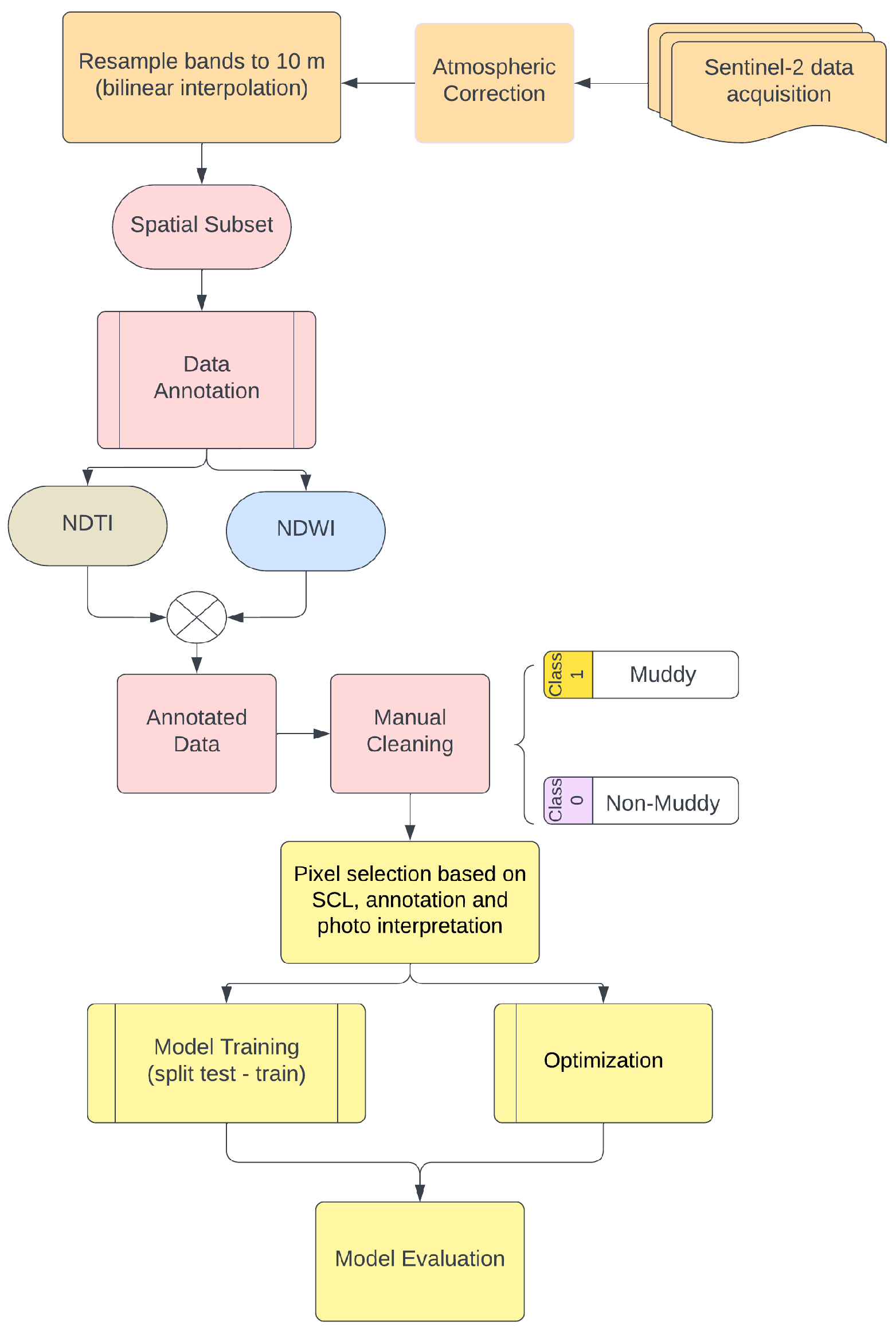
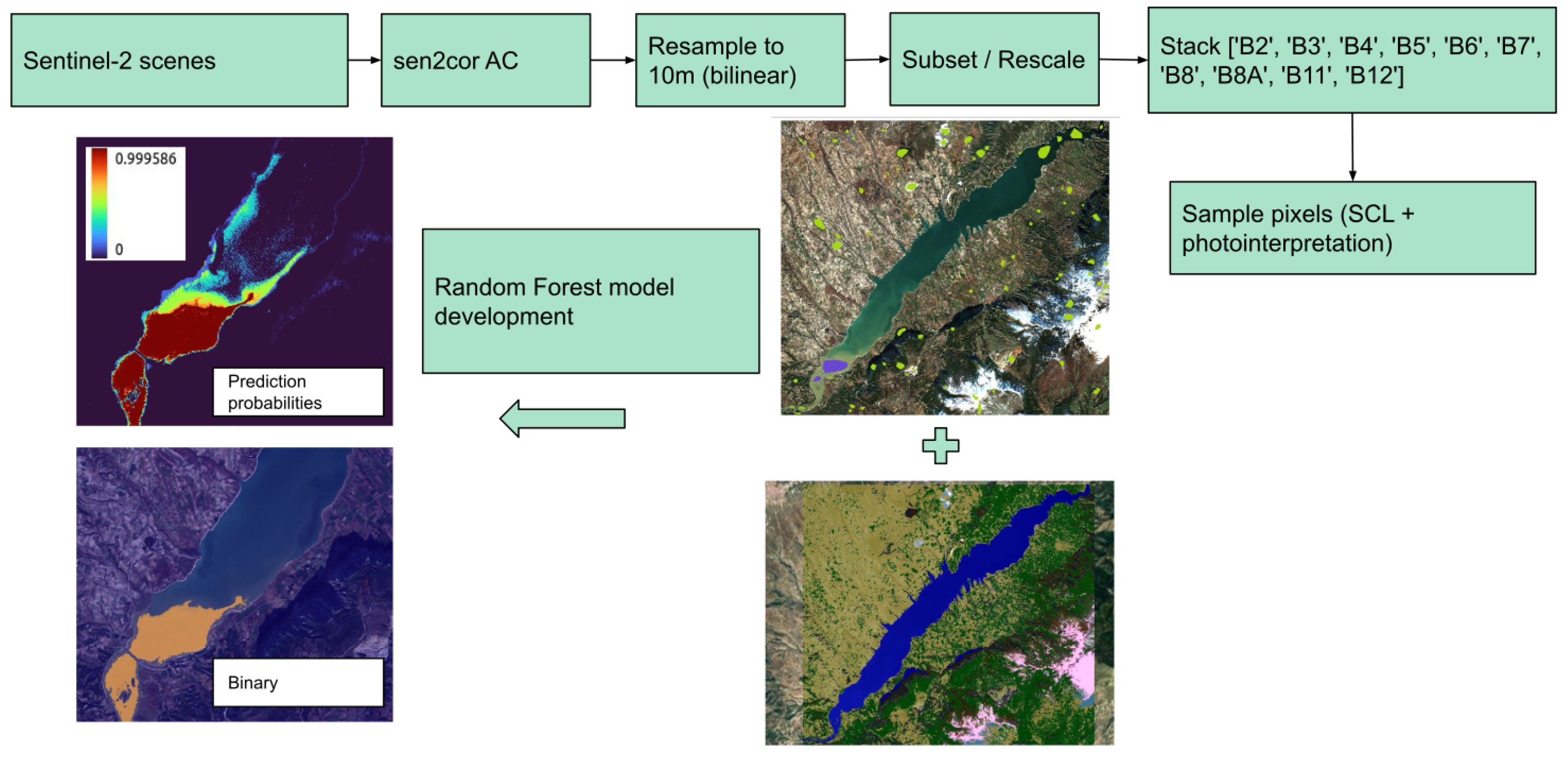
In this section, we present the steps followed from data pre-processing to data annotation and model training and evaluation. In Figure 1 we summarize the process.
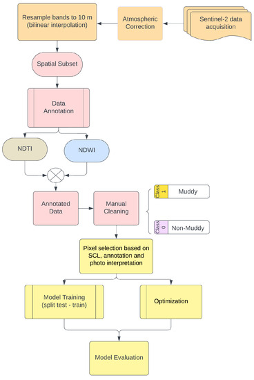
Figure 1.
Flowchart depicting the steps followed in the paper.
2.1. Selected Areas of Interest
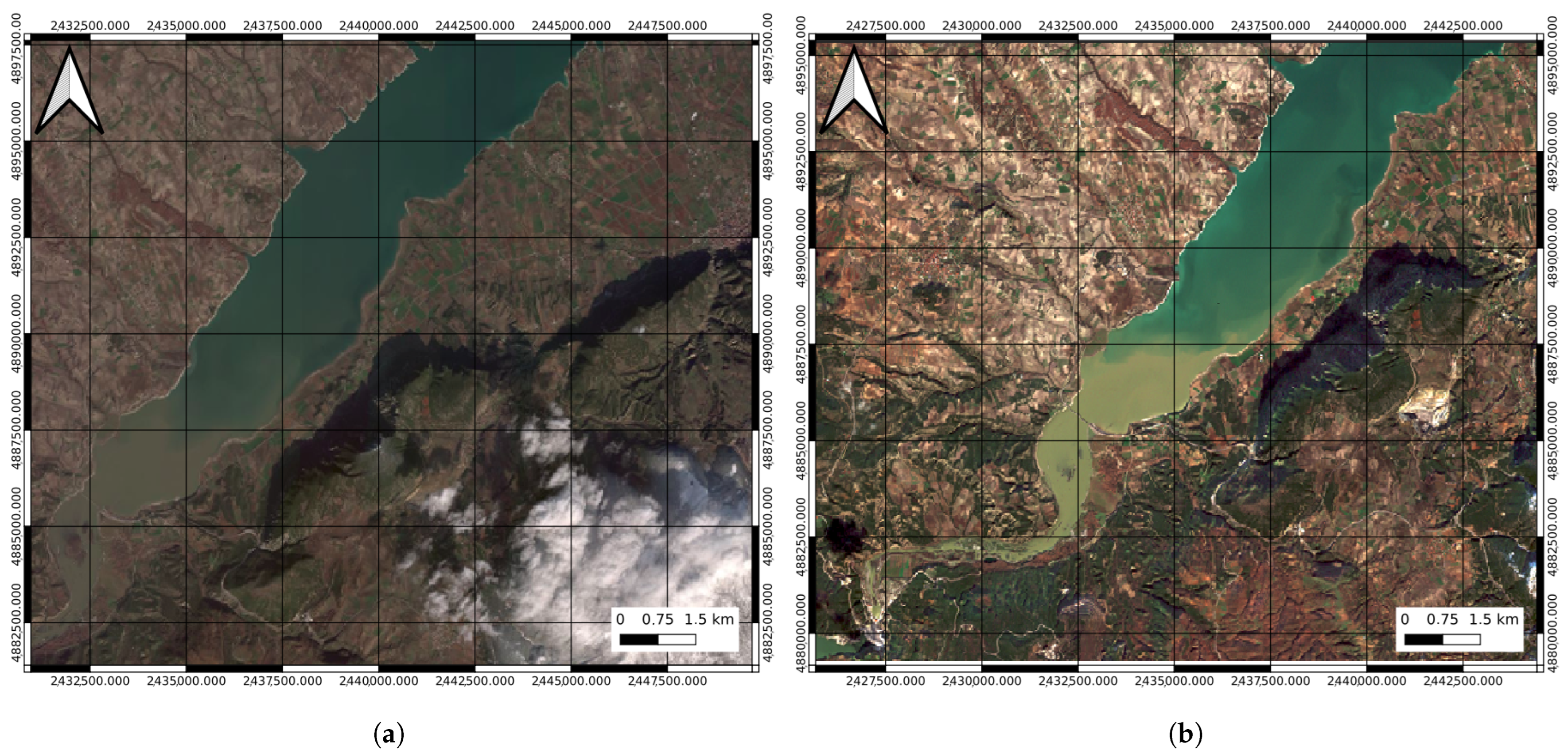
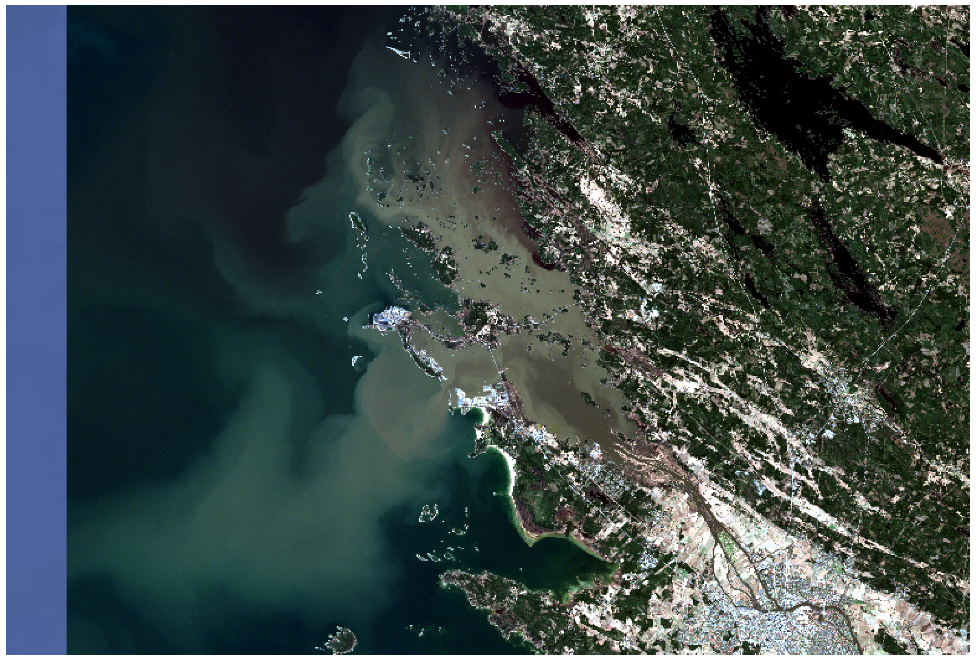
Our work focused on specific areas of interest (AOIs) from Greece and Finland which showcase different types of muddy water events as outlined in Table 1. In particular, concerning the Italian AOI (Giaretta 1), we were provided with in situ measurements along the river which were to be used for validation during the annotation process (see below), but they did not give any added value to our research. An important disadvantage was their acquisition frequency which was about 4 months apart. On the other hand, we exploited rainfall time-series to detect potential dates with heavy precipitation, which is usually coupled with high sediment load in water bodies. More useful in our first exploration were the Very High Resolution (VHR) images which we used for validation and visual comparison with Sentinel-2 data, thus confirming the presence of muddy waters. An example of a VHR and the closest Sentinel-2 (L2A) image can be seen in Figure 2 which depicts a muddy water event in the Polyphytos reservoir.

Table 1.
Information about the AOIs that were used to derive training samples for the model development.
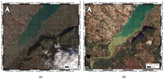
Figure 2.
(a) image showing a WorldView-3 quicklook image acquired on 15 December 2021; (b) image showing a Sentinel-2 image acquired on 19 December 2021.
In our work, the Sentinel-2 data were used for the following reasons: (1) the data is provided free of charge, (2) its characteristics make it the appropriate data to use as the spatial resolution is high enough to perform identification and classification of muddy water parts, (3) the temporal resolution (∼5 days) makes it ideal for monitoring, as the muddy water effect does not change rapidly and (4) the Sentinel-2 sensors provide us with 13 bands, which are more than enough to conduct our study.
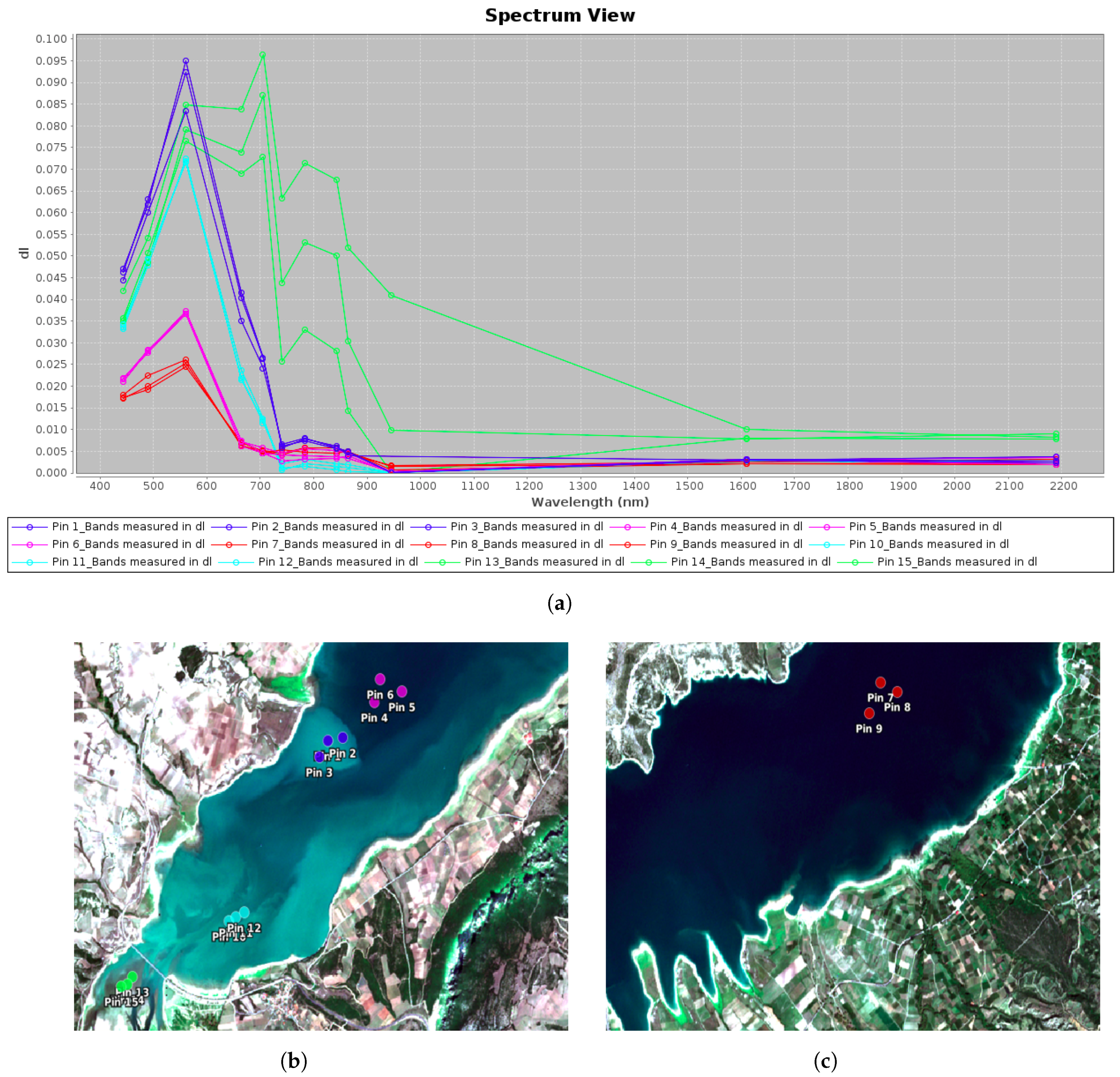
Next, we selected several pixels from several regions which seemed to have a variable content of suspended sediment using SNAP and performed a comparison of the spectral signatures between the two ends of muddy water presence, i.e., from fully clean water to water with significant sediment content (according to the identified events) (Figure 3). The reason for this first comparison was to gain an insight into the differences between the various turbidity values and their respective spectral pattern, which assisted in the evaluation of the annotated data (see below chapter). From this comparison it is evident that the sediment-laden waters show an increase in surface reflectance below roughly 1000 nm compared to clean water, while there is stability over about 1000 nm.
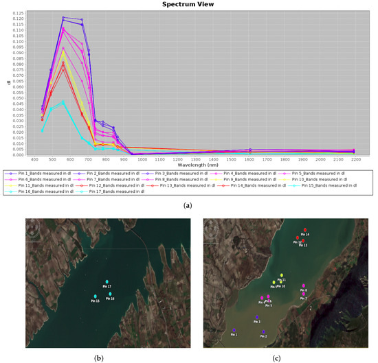
Figure 3.
A comparison of spectral signatures from various pixels in the lake with different levels of suspended sediment content as derived from Sentinel-2 (L2A). Cyan shows very little to no sediment content, while blue shows very high sediment content, based on photointerpretation. (a) Spectral signatures of Polyphytos’ pixel samples, (b) pixel samples from clean to very little sediment-laden waters, (c) pixel samples of waters with variable suspended sediment concentrations.
One challenge was determining how to distinguish between waters with lower suspended sediment content, which most often coincide with lower turbidity values, and water with higher suspended sediment content, which most often coincide with higher turbidity values. In other words, the challenge lies in discerning where one can draw a line (or decision boundary) between lows and highs of sediment content, and where the very large values are to be considered as “muddy”. Additionally, another challenge is to avoid the misidentification between waters with low/medium sediment content and turbid waters as much as possible, which occur due to reasons other than suspended sediment (e.g., from organic origin). To partly investigate this, we explored clean waters and turbid (identified by photointerpretation) waters in another Polyphytos case on 31 August 2021 (Figure 4). We noticed a similarity between spectral responses between turbid (Figure 4 category 2) and mixed/half muddy (Figure 3 category 2) and, of course an evident difference with what we call “muddy water” which consists of high suspended sediment content.

Figure 4.
Spectral responses from clear water (red, purple), turbid water (blue, cyan) and land (green) derived from a Sentinel-2 image acquired on 31 August 2021 over Polyphytos lake. (a) Spectral signatures of clean and turbid waters, (b) samples from turbid (potentially muddy) waters, (c) samples from clean waters.
Finally, another challenge that we had to combat is the choice of the Atmospheric Correction (AC) algorithm. For this reason, we tested four different ACs in two muddy water cases (19 December 2021, 24 December 2021) on data from Polyphytos, as can be seen in the Section 3. Since this is a deep research problem on its own and based on the prior exploration we showed above, we selected the simplest AC algorithm—sen2cor—as applied in the L2A products.
2.2. Data and Pre-Processing
The data that were used to train the ML model were based on the Sentinel-2 images of three different regions: Greece (one muddy water event from Polyphytos reservoir), Italy (one muddy water event from Giaretta lake and two events from nearby coastal areas) and Finland (two muddy water events in Pori and Salo). This means that data from six different scenes were used in total. The information from the scenes can be found in the Table 1 which span three epochs (autumn, winter, spring).
The pre-processing steps were followed for all Sentinel-2 scenes as follows: (a) sen2cor atmospheric correction application, (b) resample all bands to 10 m using bilinear interpolation, (c) subset and rescale the DN values dividing by 10,000, and finally (d) stack all bands that were originally in 10 m and 20 m pixel size, i.e., , , , , , , , , , . All steps were realized with SNAP Sentinel Toolbox (https://step.esa.int/main/download/snap-download/, accessed on 24 August 2023). After pre-processing, we followed the annotation procedures as described below.
2.3. Data Annotation
To achieve the goal of annotation, we combined two normalized difference spectral indices: the Modified Normalized Water Index (MNDWI) [35] and the Normalized Turbidity Index (NDTI) [36]. The MNDWI is a modified version of NDWI [37] and is better at suppressing the background noise of built-up areas, which is useful for urban and suburban areas of study. The index uses the Middle Infrared (MIR) band that substitutes Near-Infrared (NIR) and the Green band, and is defined as:
The data we use are derived from Sentinel-2 MSI, while the MNDWI [35] used the MIR band based on Landsat band 5. Therefore, the corresponding Sentinel-2 band for MIR is = 1610 nm, whereas the green band is the = 560 nm (Table 2). Therefore, MNDWI for Sentinel-2 becomes:
Table 2.
Available Sentinel-2 spectral bands 1.
The NDTI uses the red and green spectral bands to measure the amount of turbidity on small water bodies and the research is based on multi-spectral high-spatial resolution images of 10 m, provided by the SPOT-5. This resolution matches Sentinel-2 and the corresponding bands are = 665 nm for red and = 560 nm for green, thus NDTI becomes:
The computations of each index are performed in a pixel-wise sense. As a first step, we set a threshold to both MNDWI and NDTI, then we subtract the values of the MNDWI mask from those of the NDTI mask. The last step is to assign the value 0 to the regions that are not muddy, so whatever is not muddy, that is 1, becomes 0. Thus, we arrive at two classes: muddy water and non-muddy water. The results of the exploration and combination of indices can be found in the Section 3.
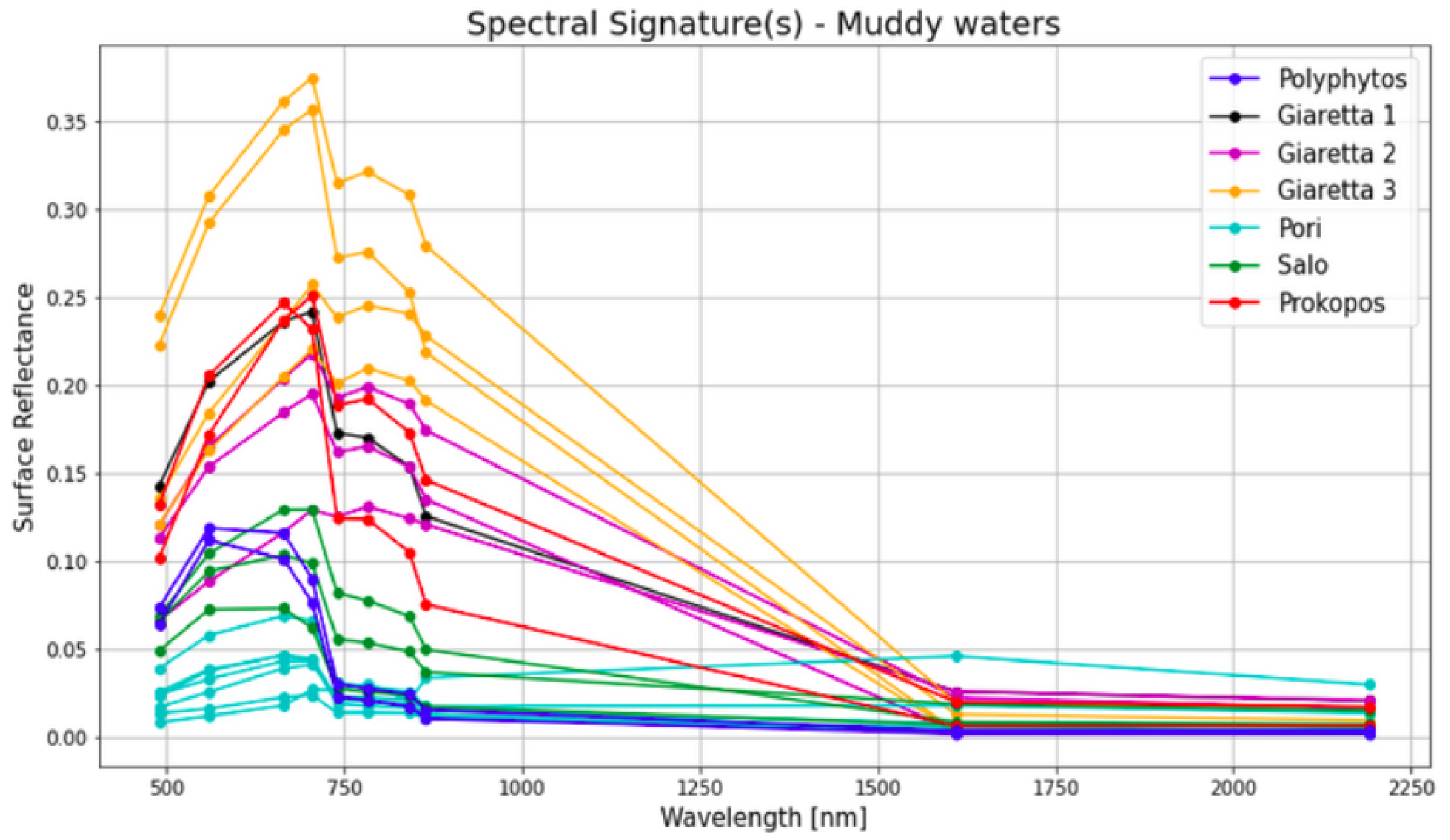
Following the annotation, we investigated the average values of spectral signatures per AOI per polygon (Figure 5) in order to assess the quality of the annotation. In the figure we notice the distinctive spectral signature pattern which shows an increase in values in all bands below (not including) SWIR1. Therefore, we can conclude that the muddy water pixels from the various polygons and AOIs show a characteristic pattern in general. In particular, Pori (in Finland, Figure 6), shows a somewhat different pattern in the visual spectrum which might be owed to the organic content in muddy waters (characteristic very dark brown color) or the generally different type of sediment.

Figure 5.
Average spectral signatures of the annotation of various AOIs uses in training and testing of the RF model.

Figure 6.
Pori AOI in Finland showing very dark brown type of muddy waters.
2.4. Model Development
From the categorical outputs that include muddy and non-muddy classes, a remote sensing expert in photointerpretation selected several polygons of variable sizes from different regions of each image from the muddy and non-muddy water classes, whose pixels were used to construct the training dataset with the additional help of the Scene Classification Layer (SCL) that is generated by sen2cor AC. SCL is a land cover classification layer included in the L2A products. The general framework up to the point of ML model development can be seen in Figure 7.

Figure 7.
General framework from data up to Random Forest model application on Sentinel-2 data.
For our model development, we selected Random Forest (RF) which is considered a powerful ML model and has been used in remote sensing extensively. It is recommended especially in tabular data formats, such as in our case, not images or time series (despite that, there is also research on these types of data). Therefore, starting the model development workflow, we selected 166,738 pixels in total which belong to all aforementioned AOIs, after undersampling the negative (non-muddy water) class in order to achieve a class balance between muddy and non-muddy water classes which is crucial for the ML model development. In turn, those were randomly split into training and test sets with 133,390 and 33,348 pixels, respectively. In the training samples we included several classes relevant to land such as bare soil, green vegetation, brown vegetation, different crops, bare rocks, as well as clean water and clouds.
After selecting the training and test sets, we perform an optimization based on Grid Search to derive the best possible hyperparameters for our RF model. The hyperparameters we try to find optimal values for are (a) number of trees (b) tree depth and (c) class balance. In Table 3, we summarize the possible number of values we used for the Grid Search with bold being the ones selected as optimal.
Table 3.
Values of hyperparameters of the Random Forest model that were tested during Grid Search.
To find the optimal numbers, we performed a five-fold cross validation with 5 repeats based on the F1-score classification metric, which resulted in 7425 total model fits.
3. Results and Discussion
3.1. Model Application and Evaluation
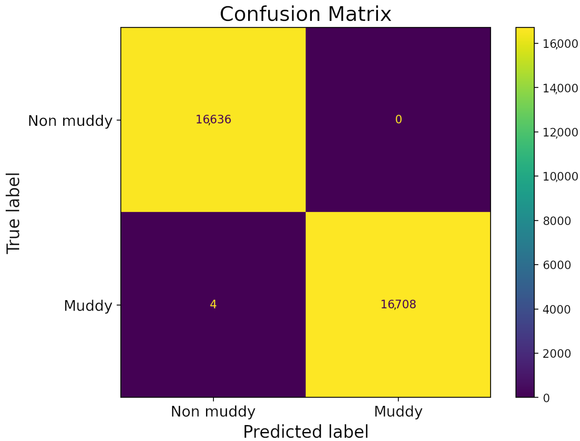
Concerning the model evaluation after optimizing it, in order to further assess the results, we first examined the feature importances that are derived from the RF model which are inherently produced, and secondly we applied the optimized model to other AOIs. This way we are able to assess the true performance of the model in the so-called unseen cases, which are data that have not been used in the training procedure. The unseen data include the test set also for which we derived several accuracy metrics along with the training set, such as Accuracy, Recall, Precision, F1-score and Receiver Operating Characteristic-Area Under Curve (ROC-AUC). All metrics achieved a performance of over 98% as shown in the confusion matrix in both training and test sets (Figure 8).

Figure 8.
Confusion matrix concerning the test set when applying the optimized RF model.
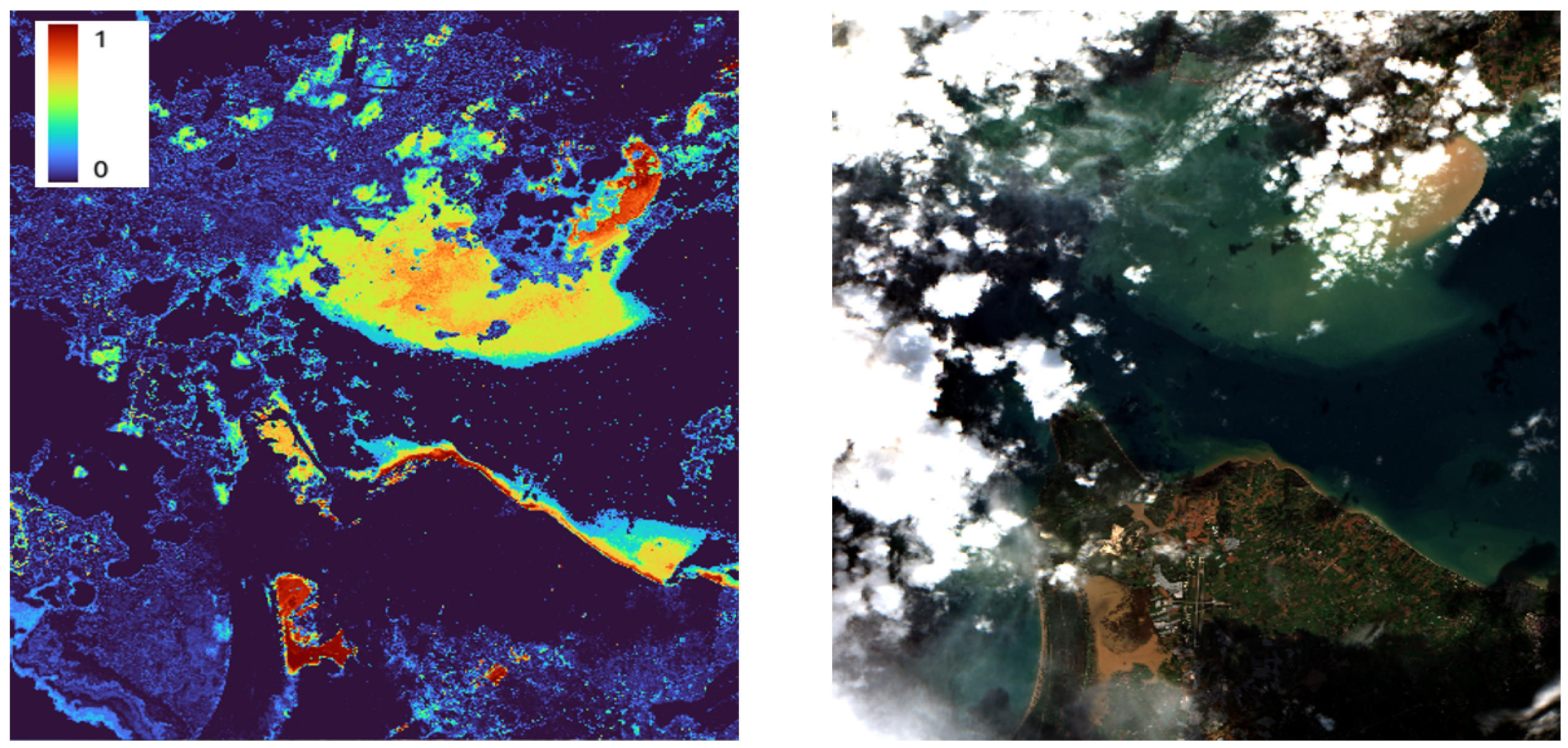
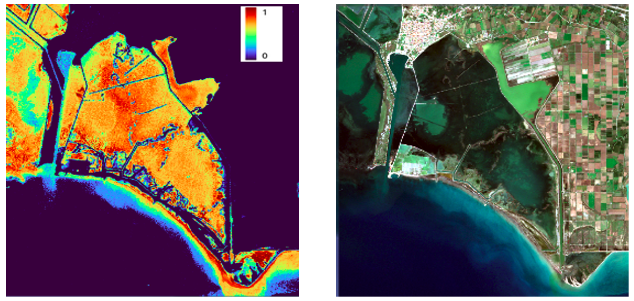
After applying our RF model to cases with similar muddy water characteristics such as in Prokopos (Greece), we notice an adequate performance (Figure 9). However, this does not seem to be the case when we apply the model in regions with shallow waters and high chlorophyll content (Figure 10), where an overestimation can be observed. Therefore, we conclude there might be cases that the model would overestimate and probably underestimate in muddy water types that exist and have not been included in the training dataset from other AOIs and events.

Figure 9.
Right figure shows the RGB in Prokopos region in western Greece on 25 September 2021. Left figure shows the same region as expressed by prediction probabilities of the RF model output. The performance of the models seems adequate, although with relatively high prediction probabilities in water with lower/medium suspended sediment content.

Figure 10.
Right figure shows Sentinel-2 RGB of Mesologgi region (western Greece) on 4 November 2021. Left figure shows RF model prediction expressed in prediction probabilities of the same region.
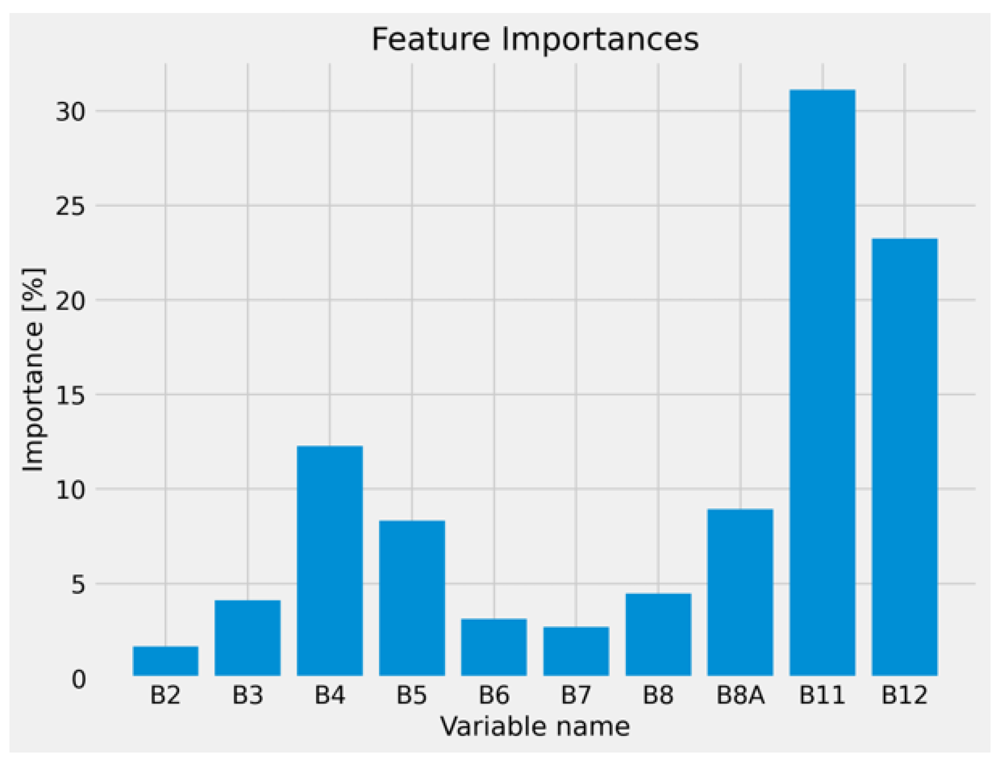
Regarding the feature importances, we notice the biggest contributions from , , , , (Figure 11). Especially, the contribution from and can be attributed to the presence of several land classes and clouds in the training dataset. All available bands of Sentinel-2 data used can be seen in Table 2.

Figure 11.
Feature importances derived from the RF algorithm.
3.2. Atmospheric Corrections
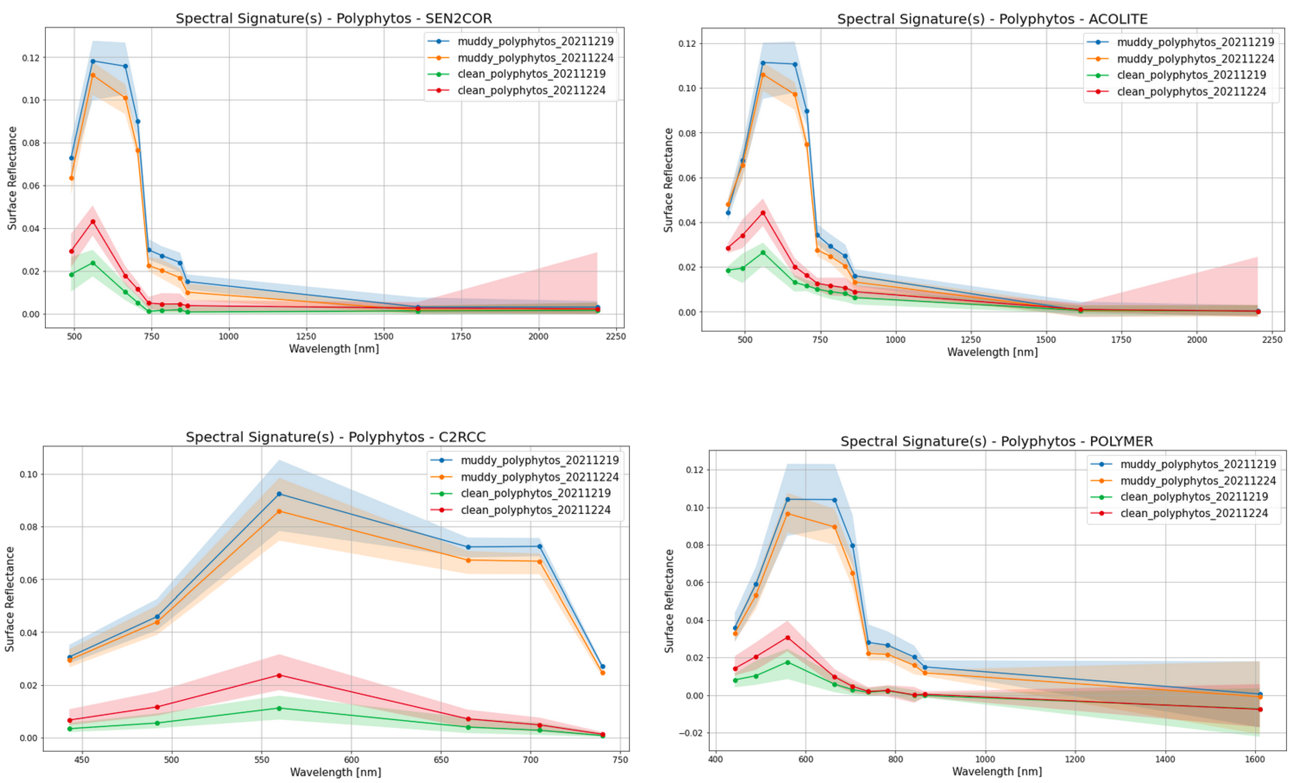
Regarding the Atmospheric Correction, the three ACs (polymer (https://www.hygeos.com/polymer, accessed on 24 August 2023), ACOLITE (https://odnature.naturalsciences.be/remsem/software-and-data/acolite, accessed on 24 August 2023) and C2RCC (https://c2rcc.org/, accessed on 24 August 2023)) were performed on L1C products, while the fourth AC (sen2cor (https://step.esa.int/main/snap-supported-plugins/sen2cor/, accessed on 24 August 2023)) was already applied on the L2A product. The results, with the appropriately scaled RGBs, can be seen in Figure 12 (right), and the spectral response of muddy waters and clean waters were investigated qualitatively (see Figure 12 and Figure 13). It is noticeable that in the case of sen2cor, polymer and ACOLITE ACs the relative difference of the spectral response between muddy and clean waters is similar, while this is not the case for C2RCC. In addition, not all ACs give all spectral bands as a corrected output which we consider as a drawback especially in the case that we would like to include different land and cloud classes in our ML approach.
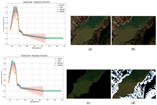
Figure 12.
Right figure shows the appropriately scaled RGBs of the four different ACs applied for one muddy water case in Polyphytos. Left figures show the spectral response from muddy waters only, for two dates in Polyphytos for the four different ACs. (a) sen2cor, (b) Acolite, (c) c2rcc, (d) Polymer.
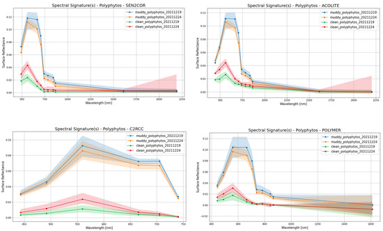
Figure 13.
The spectral response of muddy and clean waters from the four ACs.
In addition, based on these figures, the relative difference between muddy water spectral responses among all ACs seem to be stable. In our problem, this essentially means that what we would need is not a perfect AC algorithm that would give almost ground truth (if possible) surface reflectances, but an AC algorithm that does not significantly decrease the relative difference of surface reflectance among the different classes.
3.3. Data Annotation
Regarding data annotation with the index combination, the first attempt is focused on MNDWI. This index is good enough in water body identification, albeit it fails to recognize the muddy water parts. Consequently, we call on the Normalized Difference Turbidity Index (NDTI), which succeeds at identifying muddy waters, however the noise produced is significant. Finally, taking a closer look at the results of both indices (Figure 14 and Figure 15), we attain insight into their capability of combining to achieve the suppression of background noise, and we manage to classify the muddy water pixels.

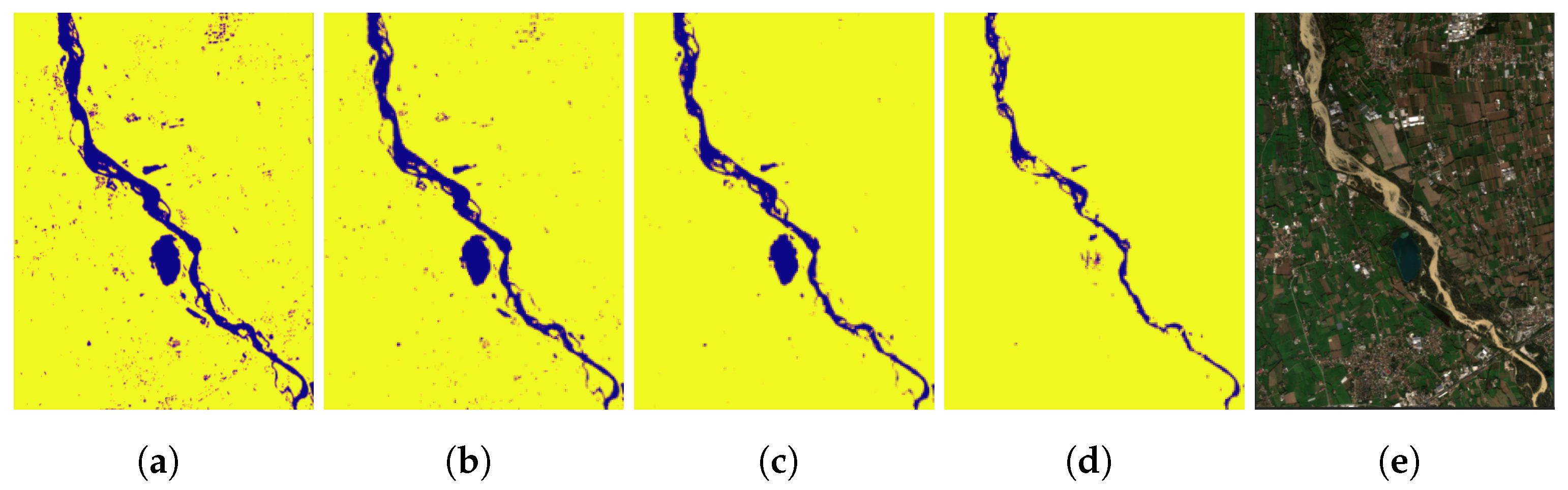
Figure 14.
Different threshold values of the MNDW index for the Giaretta region. (a) threshold = −0.1, (b) threshold = 0, (c) threshold = 0.2, (d) threshold = 0.5, (e) Giaretta.

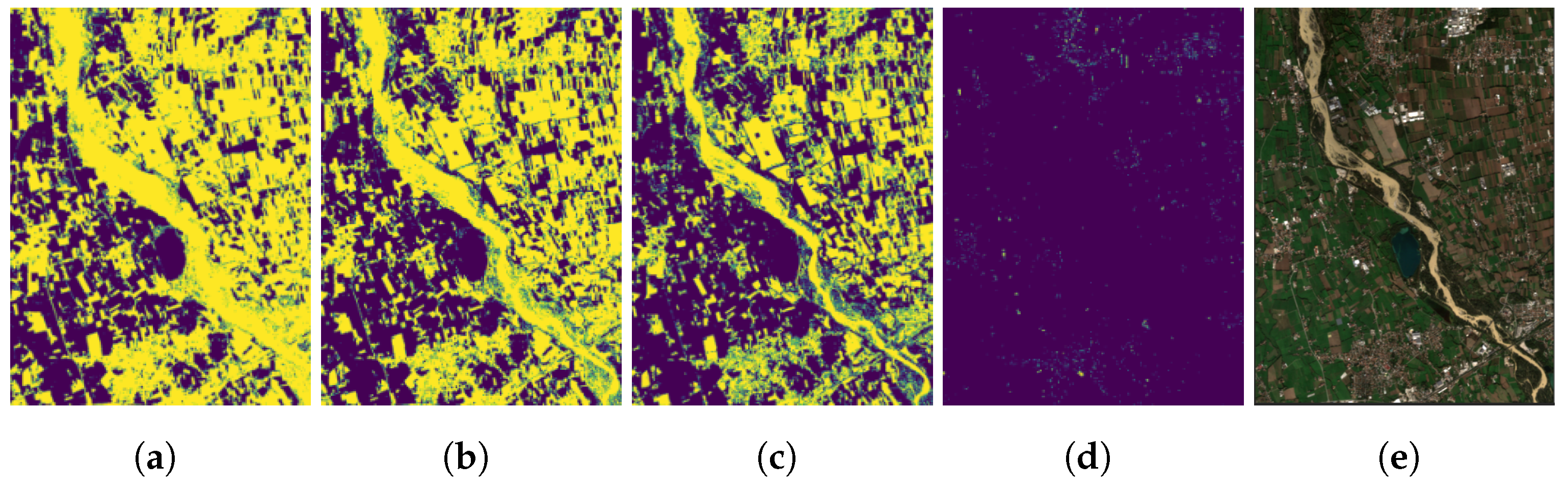
Figure 15.
Different threshold values of the NDT Index for the Giaretta region. (a) threshold = −0.5, (b) threshold = −0.1, (c) threshold = 0, (d) threshold = 0.2, (e) Giaretta.
As the first step for MNDWI, we must put an appropriate threshold value on the MNDWI < threshold to create a binary mask. Although it is a good index regarding water detection, it fails to recognize muddy waters as we can see in the results for different threshold values in Figure 14.
As can be seen by the results, for index < threshold, negative values lead to high noise, whilst more positive values suppress the noise substantially, at the cost of low-quality characteristics. The choice of the optimal threshold value is subjective and relies on the region of interest, due to differences in the composition of the water and land. As previously mentioned, this method does not yield the expected results, although as we will see it can be used in combination with the next index.
After failing at distinguishing muddy waters with the MNDWI, we continue with the turbidity index. Applying some threshold values, this time on NDTI > threshold, we obtained the results in Figure 15.
Upon inspecting the results, we ascertain that this index manages to identify muddy water regions and separate them from clean water parts, albeit the noise by false muddy waters is very high. In order to obtain the best results, we choose threshold values ranging from slightly negative to slightly positive. Again, we cannot give a final value as the choice depends on one’s knowledge of muddy waters, but also the values vary among different AOIs. Following, we examine the combination of the two indices discussed so far.
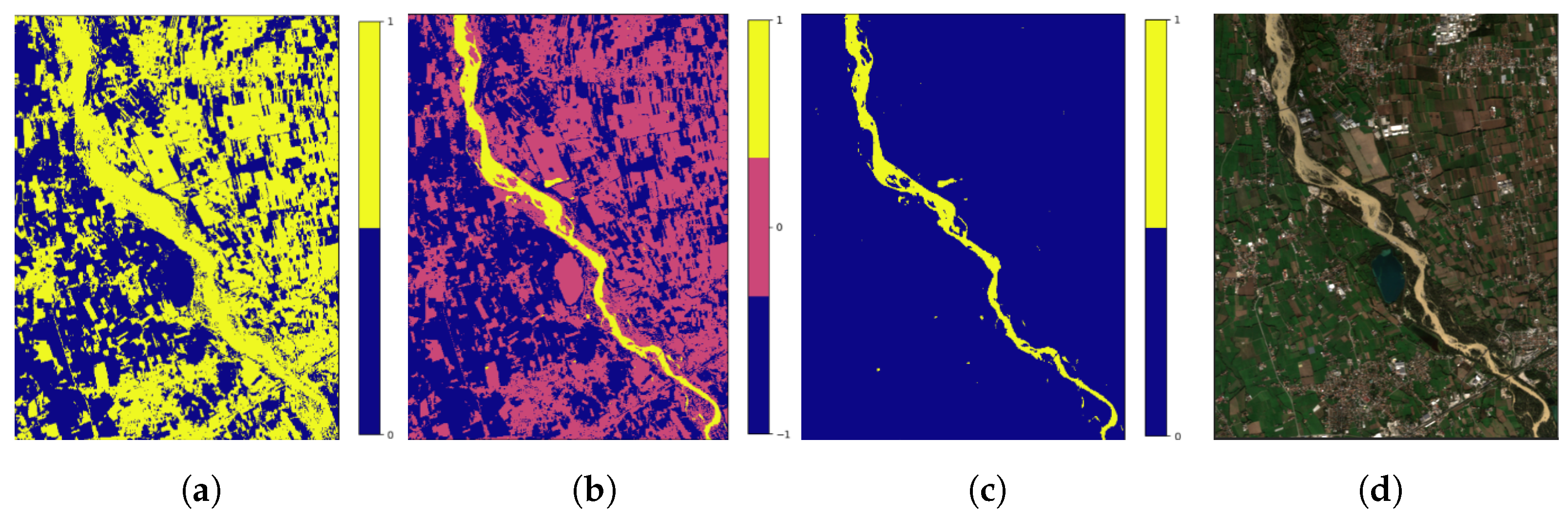
The test of the above indices did not yield the expected results, that is, the distinction of the water regions occupied by mud. However, taking a closer look at both methods’ noise parts, we discern some similarities and thus we obtain the insight of combining these two to eliminate the noise. The steps of annotating the muddy water parts of an image using the index combination can be seen below (Figure 16). For the specific results, the threshold values are for NDTI and for MNDWI.

Figure 16.
Index combination steps for the Giaretta region. (a) initial NDTI mask, (b) NDTI - MNDWI mask, (c) final mask, (d) Giaretta.
The results obtained using the method of index combination are gratifying, but there are some problems or limitations arising. To begin with, for the region of Polyphytos (Figure 17), where snow is present, we encounter additional noise. Additionally, the same applies for the case of clouds in the image. This makes the use of manual cleaning of these parts mandatory, as no threshold value combination can remove them. This unfortunately applies for the noise in general, making it unavoidable to use manual labor, but we will see that we can circumvent it to some extent. Except for that, the other caveat is the subjective nature of the method, as it relies on one’s photointerpretation skills. The expert photointerpretation relies on the researcher’s previous knowledge on muddy waters. Of course, the results of the expert are not 100% accurate as they are based on satellite images, but also edge cases such as single ambiguous pixels cannot be assigned values easily, so there is some uncertainty. Assuming that a validation/comparison on the expert’s choices could be made, then in situ or drone measurements should have been provided on each specific AOI, at the same time of the satellite passing. However, very often, this is not feasible as it requires many resources (human, financial, timing etc.) and coordination. Therefore, since validation of the expert’s selection is unfeasible, we consider it as one of the least unsuitable approaches.
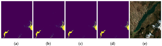
Figure 17.
Different index threshold combinations for the Polyphytos region. (a) MNDWI = 0.7, NDTI = −0.1, (b) MNDWI = 0.7, NDTI = −0.2, (c) MNDWI = 0.8, NDTI = −0.1, (d) MNDWI = 0.8, NDTI = −0.2, (e) Polyphytos.
Furthermore, the threshold values depend on each separate region, making it impossible to extract an optimal value combination to apply to the whole dataset, as the differences in composition and photo capturing conditions vary for each region. This limitation prevents us from creating a fully automated annotation technique. Finally, another limitation that applies to all techniques is the satellite’s spatial resolution. Although a 10 m × 10 m resolution is high, it limits the results of all methods. To proceed with the manual cleanup using QGIS, we converted the raster results to vectors. The final two classes are then distinguished. The first one is the muddy water class, with pixel values of 1. The second class includes the bare soil, clean water, vegetation, snow, clouds, algae, etc., and is named as non-muddy, with pixel values of 0.
Alternative Annotation Approaches
Another annotation approach that can be used for defining muddy water and non-muddy water classes is exploiting the information derived from water quality parameters in the following or a similar way: calculate water quality parameters on the Sentinel-2 images, such as turbidity and/or total suspended matter and define a threshold value generating the two desired classes. The threshold value could be either data-driven or end-user/expert-driven. The former could be based on the statistical distribution of one or both of the water quality parameters, while the latter could be based on a subjective or quasi-objective value that would have a physical meaning. However, calculating water quality parameters requires the choice of an appropriate atmospheric correction algorithm resulting in very high accuracy/precision of pixel surface reflectance. Since such a universal atmospheric correction algorithm that would work equally well under all conditions does not currently exist, this means that the biases that were aimed to be overcome in the first place would still exist. Despite that such an approach needs more detailed study, in our work we suggest that an ensemble annotation approach would minimize biases.
3.4. Limitations
One important limitation of our approach is the dataset size and variability. By putting explainable AI into practice in the sense of experimenting with the impact of including different land cover and water quality pixels in the training dataset and assessing its impact on the prediction outcomes, as well as enhancing the quality of the current training dataset, we still notice the presence of Type I errors/false positives and Type II errors/false negatives when applying the model to more unseen muddy water cases. Thus, this means that the models would need retraining in certain cases (and not always) where the unseen muddy waters are composed of sediment particles which are very different to the ones the model is trained on. Another limitation pertains to the annotation approach which demands different threshold combinations in each area of interest, preventing us from creating a fully automatic procedure, that is a universal threshold value combination for all input data.
3.5. Random Forest vs. Convolutional Neural Networks
Random Forest and Convolutional Neural Networks (CNNs) are two radically different approaches for handling image data. Random Forest has proven its effectiveness and ease of use for classification tasks in remote sensing [38,39] and thus can be the initial choice when combating a classification problem. Usually when using Random Forest, the data are treated as tabular, namely, considering pixels as single entities. On the other hand, the progress of technology and access to computational resources led to the wide adaptation of deep learning techniques, and especially CNNs. CNNs can exploit satellite images almost to the fullest extent, since they can be treated as image patches. We stress that the adaptation of CNNs in the muddy water problem will offer new opportunities in exploiting big satellite data and the generation of benchmark datasets towards constructing geographically universal classifiers. Some of the main differences and drawbacks of Random Forest (or generally traditional machine learning) compared to CNNs are briefly described below:
- Lack of Spatial/Spectral/Temporal Information: Random Forest generally treats each pixel as an independent data point not considering spatial autocorrelation among neighboring pixels and spectral autocorrelation among bands per pixel, while this is not the case for CNNs as the can implement convolution operations in both spatial, spectral or even temporal dimensions at once or separately.
- Feature Engineering: Random Forest relies on handcrafted features or raw pixel values, which may not capture complex hierarchical features in the data as effectively as CNNs, thus it heavily depends on feature engineering, where domain expertise is required. On the other hand, CNNs automatically learn hierarchical features from the image data reducing the need for extensive feature engineering, which would allow for an easier build of end-to-end learning architectures.
- Scalability: Random Forest can be computationally expensive when applied to large-scale image datasets, as it involves building and maintaining multiple decision trees. CNNs can be more scalable for image processing tasks because they utilize shared weights and feature maps, making them more efficient for large images.
3.6. Prospect and Usability
The proposed approach of muddy water mapping which is based on semantic segmentation does not aim to substitute the the typical water quality parameter retrieval approaches. In an operational setting and depending on the purpose of use, it can have the advantages of low latency of product generation (e.g., no need for specialized time-consuming atmospheric correction), it can be sensor-independent and a model could be easily updated by exploiting transfer learning (assuming deep learning-based model usage). In the case of the RF approach and the non-variable enough dataset, the model can be retrained on a new AOI in order to deliver valid products to an end-user. Thus, such a product/service can be integrated in water management and decision support systems, as is the case for the proposed approach of the current work as a pilot (https://portal-wqems.opsi.lecce.it, accessed on 24 August 2023). An end-user may only need the information of whether such an extreme event occurs or not, the geometrical features and extent, and an indirect visual estimation of sediment content (derived by the prediction probabilities) which are essential for the emergency response. From a research perspective, unknown regions and water bodies of muddy water presence can be identified around the world (assuming a highly variable training dataset).
3.7. Suggestions for Monitoring Improvements
The potential that came with open and free Copernicus data is undeniable. Copernicus satellite missions such as Sentinel-2 and Sentinel-3 can provide both high spatial and temporal resolutions, although not at the same time, since Sentinel-3 comes with almost daily measurements but low spatial resolutions (∼300 m) (https://sentinels.copernicus.eu/web/sentinel/user-guides/sentinel-3-olci/resolutions/spatial, accessed on 24 August 2023) while Sentinel-2 comes with high spatial but lower temporal resolution. In addition, recent years have shown an emerging interest in the adaptation of deep learning (and especially CNN-based) approaches for the downscaling task by sensor fusion (e.g., [40]). Therefore, we suggest that the monitoring of muddy waters in the context of this work could be improved by the wider adaptation and fusion of Sentinel-2 and Sentinel-3 missions, and the development of deep learning downscaling approaches to generate water quality products of high both temporal and spatial resolution.
4. Conclusions
In conclusion, our work focuses on the mapping/detection of muddy waters through a machine learning-based semantic segmentation approach for inland drinking water reservoirs with a spatial resolution of 10 m using Sentinel-2 satellite data. The task at hand is fairly new and requires further research, especially in the part of generating annotations and a more variable training dataset. The model we developed is a Random Forest model used on data in a tabular format; based on the training dataset we used, it performs fairly well. This means that there is room for improvement from the proper dataset generation side which would offer maximal generalization capabilities. With increasing complexity there is demand for more complex models, thus, we foresee a future utilization of image-based deep learning approaches such as CNNs.
Author Contributions
Conceptualization, I.G. and A.M.; methodology/software/validation/formal analysis/visualization, K.V. and C.P.; investigation, K.V.; resources, A.M. and I.G.; data curation, K.V.; writing—original draft preparation, K.V. and C.P.; writing—review and editing, K.V., C.P. and A.M.; supervision, I.G. and A.M.; project administration, S.V. and I.K.; funding acquisition, S.V. and I.K. All authors have read and agreed to the published version of the manuscript.
Funding
This research was funded by the European Commission through the H2020 WQeMS project under Grant Agreement ID No 101004157 and Horizon Europe project PERIVALLON under Grant Agreement ID No 101073952.
Institutional Review Board Statement
Not applicable.
Informed Consent Statement
Not applicable.
Data Availability Statement
Not applicable.
Conflicts of Interest
The authors declare no conflict of interest.
Abbreviations
The following abbreviations are used in this manuscript:
| AOI | Area Of Interest |
| ML | Machine Learning |
| AC | Atmospheric Correction |
| SCL | Scene Classification Layer |
| NDTI | Normalized Difference Turbidity Index |
| MNDWI | Modified Normalized Difference Water Index |
| RF | Random Forest |
| TSS | Total Suspended Sediment |
References
- Davies-Colley, R.; Smith, D. Turbidity suspeni)ed sediment, and water clarity: A review. J. Am. Water Resour. Assoc. 2001, 37, 1085–1101. [Google Scholar] [CrossRef]
- Bilotta, G.S.; Brazier, R.E. Understanding the influence of suspended solids on water quality and aquatic biota. Water Res. 2008, 42, 2849–2861. [Google Scholar] [CrossRef] [PubMed]
- Albering, H.J.; Rila, J.P.; Moonen, E.; Hoogewerff, J.A.; Kleinjans, J. Human health risk assessment in relation to environmental pollution of two artificial freshwater lakes in The Netherlands. Environ. Health Perspect. 1999, 107, 27–35. [Google Scholar] [CrossRef] [PubMed]
- Mingzhou, Q.; Jackson, R.H.; Zhongjin, Y.; Jackson, M.W.; Bo, S. The effects of sediment-laden waters on irrigated lands along the lower Yellow River in China. J. Environ. Manag. 2007, 85, 858–865. [Google Scholar] [CrossRef] [PubMed]
- Mann, A.G.; Tam, C.C.; Higgins, C.D.; Rodrigues, L.C. The association between drinking water turbidity and gastrointestinal illness: A systematic review. BMC Public Health 2007, 7, 256. [Google Scholar] [CrossRef]
- Schwartz, J.; Levin, R.; Goldstein, R. Drinking water turbidity and gastrointestinal illness in the elderly of Philadelphia. J. Epidemiol. Community Health 2000, 54, 45–51. [Google Scholar] [CrossRef]
- Gauthier, V.; Barbeau, B.; Tremblay, G.; Millette, R.; Bernier, A.M. Impact of raw water turbidity fluctuations on drinking water quality in a distribution system. J. Environ. Eng. Sci. 2003, 2, 281–291. [Google Scholar] [CrossRef]
- Richter, B.D.; Braun, D.P.; Mendelson, M.A.; Master, L.L. Threats to imperiled freshwater fauna: Amenazas a la fauna dulceacuicola en riesgo. Conserv. Biol. 1997, 11, 1081–1093. [Google Scholar] [CrossRef]
- Henley, W.; Patterson, M.; Neves, R.; Lemly, A.D. Effects of sedimentation and turbidity on lotic food webs: A concise review for natural resource managers. Rev. Fish. Sci. 2000, 8, 125–139. [Google Scholar] [CrossRef]
- Hollis, E.H.; Boone, J.G.; DeRose, C.R.; Murphy, G.J. A Literature Review of the Effects of Turbidity and Siltation on Aquatic Life; Unpublished Staff Report; Department of Chesapeake Bay Affairs: Annapolis, MD, USA, 1964.
- Dunlop, J.; McGregor, G.; Horrigan, N. Potential Impacts of Salinity and Turbidity in Riverine Ecosystems. National Action Plan for Salinity and Water Quality; Technical Report, WQ06 Technical Report. QNRM05523; The National Action Plan for Salinity and Water Quality (NAPSWQ): Queensland, Australia, 2005.
- Yang, H.; Kong, J.; Hu, H.; Du, Y.; Gao, M.; Chen, F. A review of remote sensing for water quality retrieval: Progress and challenges. Remote Sens. 2022, 14, 1770. [Google Scholar] [CrossRef]
- Toming, K.; Kutser, T.; Uiboupin, R.; Arikas, A.; Vahter, K.; Paavel, B. Mapping water quality parameters with sentinel-3 ocean and land colour instrument imagery in the Baltic Sea. Remote Sens. 2017, 9, 1070. [Google Scholar] [CrossRef]
- Shen, M.; Duan, H.; Cao, Z.; Xue, K.; Qi, T.; Ma, J.; Liu, D.; Song, K.; Huang, C.; Song, X. Sentinel-3 OLCI observations of water clarity in large lakes in eastern China: Implications for SDG 6.3. 2 evaluation. Remote Sens. Environ. 2020, 247, 111950. [Google Scholar] [CrossRef]
- Surisetty, V.V.A.K.; Sahay, A.; Ramakrishnan, R.; Samal, R.N.; Rajawat, A.S. Improved turbidity estimates in complex inland waters using combined NIR–SWIR atmospheric correction approach for Landsat 8 OLI data. Int. J. Remote Sens. 2018, 39, 7463–7482. [Google Scholar] [CrossRef]
- Ma, Y.; Song, K.; Wen, Z.; Liu, G.; Shang, Y.; Lyu, L.; Du, J.; Yang, Q.; Li, S.; Tao, H.; et al. Remote sensing of turbidity for lakes in northeast China using Sentinel-2 images with machine learning algorithms. IEEE J. Sel. Top. Appl. Earth Obs. Remote Sens. 2021, 14, 9132–9146. [Google Scholar] [CrossRef]
- Sa’ad, F.N.A.; Tahir, M.S.; Jemily, N.H.B.; Ahmad, A.; Amin, A.R.M. Monitoring Total Suspended Sediment Concentration in Spatiotemporal Domain over Teluk Lipat Utilizing Landsat 8 (OLI). Appl. Sci. 2021, 11, 7082. [Google Scholar] [CrossRef]
- Bi, S.; Li, Y.; Xu, J.; Liu, G.; Song, K.; Mu, M.; Lyu, H.; Miao, S.; Xu, J. Optical classification of inland waters based on an improved Fuzzy C-Means method. Opt. Express 2019, 27, 34838–34856. [Google Scholar] [CrossRef] [PubMed]
- Xu, H.; Xu, G.; Wen, X.; Hu, X.; Wang, Y. Lockdown effects on total suspended solids concentrations in the Lower Min River (China) during COVID-19 using time-series remote sensing images. Int. J. Appl. Earth Obs. Geoinf. 2021, 98, 102301. [Google Scholar] [CrossRef]
- Tripathi, G.; Pandey, A.C.; Parida, B.R. Spatio-temporal analysis of turbidity in ganga river in patna, bihar using sentinel-2 satellite data linked with covid-19 pandemic. In Proceedings of the 2020 IEEE India Geoscience and Remote Sensing Symposium (InGARSS), Virtual, 2–4 December 2020; pp. 29–32. [Google Scholar]
- Garg, V.; Aggarwal, S.P.; Chauhan, P. Changes in turbidity along Ganga River using Sentinel-2 satellite data during lockdown associated with COVID-19. Geomat. Nat. Hazards Risk 2020, 11, 1175–1195. [Google Scholar] [CrossRef]
- Wang, J.; Tong, Y.; Feng, L.; Zhao, D.; Zheng, C.; Tang, J. Satellite-Observed Decreases in Water Turbidity in the Pearl River Estuary: Potential Linkage With Sea-Level Rise. J. Geophys. Res. Ocean. 2021, 126, e2020JC016842. [Google Scholar] [CrossRef]
- Jensen, J.R. Digital Image Processing: A Remote Sensing Perspectives; Prentice Hall: Upper Saddle River, NJ, USA, 2005. [Google Scholar]
- Sumbul, G.; Charfuelan, M.; Demir, B.; Markl, V. Bigearthnet: A large-scale benchmark archive for remote sensing image understanding. In Proceedings of the IGARSS 2019–2019 IEEE International Geoscience and Remote Sensing Symposium, Yokohama, Japan, 28 July–2 August 2019; pp. 5901–5904. [Google Scholar]
- Tseng, G.; Zvonkov, I.; Nakalembe, C.L.; Kerner, H. Cropharvest: A global dataset for crop-type classification. In Proceedings of the Thirty-Fifth Conference on Neural Information Processing Systems Datasets and Benchmarks Track (Round 2), Virtual, 11 October 2021. [Google Scholar]
- Helber, P.; Bischke, B.; Dengel, A.; Borth, D. Eurosat: A novel dataset and deep learning benchmark for land use and land cover classification. IEEE J. Sel. Top. Appl. Earth Obs. Remote Sens. 2019, 12, 2217–2226. [Google Scholar] [CrossRef]
- Rumora, L.; Miler, M.; Medak, D. Impact of various atmospheric corrections on sentinel-2 land cover classification accuracy using machine learning classifiers. ISPRS Int. J. Geo-Inf. 2020, 9, 277. [Google Scholar] [CrossRef]
- Song, C.; Woodcock, C.E.; Seto, K.C.; Lenney, M.P.; Macomber, S.A. Classification and change detection using Landsat TM data: When and how to correct atmospheric effects? Remote Sens. Environ. 2001, 75, 230–244. [Google Scholar] [CrossRef]
- Emberton, S.; Chittka, L.; Cavallaro, A.; Wang, M. Sensor capability and atmospheric correction in ocean colour remote sensing. Remote Sens. 2015, 8, 1. [Google Scholar] [CrossRef]
- Gordon, H.R. Evolution of ocean color atmospheric correction: 1970–2005. Remote Sens. 2021, 13, 5051. [Google Scholar] [CrossRef]
- Maurya, L.; Lohchab, V.; Mahapatra, P.K.; Abonyi, J. Contrast and brightness balance in image enhancement using Cuckoo Search-optimized image fusion. J. King Saud Univ.-Comput. Inf. Sci. 2022, 34, 7247–7258. [Google Scholar] [CrossRef]
- Akbarinia, A.; Gil-Rodriguez, R. Deciphering image contrast in object classification deep networks. Vis. Res. 2020, 173, 61–76. [Google Scholar] [CrossRef]
- Guo, J.; Ma, J.; García-Fernández, Á.F.; Zhang, Y.; Liang, H. A survey on image enhancement for Low-light images. Heliyon 2023, 9, e14558. [Google Scholar] [CrossRef] [PubMed]
- Cai, T.; Zhu, F.; Hao, Y.; Fan, X. Performance evaluation of image enhancement methods for objects detection and recognition. In Proceedings of the AOPC 2015: Image Processing and Analysis, SPIE, Beijing, China, 8 October 2015; Volume 9675, pp. 732–736. [Google Scholar]
- Xu, H. Modification of normalised difference water index (NDWI) to enhance open water features in remotely sensed imagery. Int. J. Remote Sens. 2006, 27, 3025–3033. [Google Scholar] [CrossRef]
- Lacaux, J.; Tourre, Y.; Vignolles, C.; Ndione, J.; Lafaye, M. Classification of ponds from high-spatial resolution remote sensing: Application to Rift Valley Fever epidemics in Senegal. Remote Sens. Environ. 2007, 106, 66–74. [Google Scholar] [CrossRef]
- McFeeters, S.K. The use of the Normalized Difference Water Index (NDWI) in the delineation of open water features. Int. J. Remote Sens. 1996, 17, 1425–1432. [Google Scholar] [CrossRef]
- Belgiu, M.; Drăguţ, L. Random forest in remote sensing: A review of applications and future directions. ISPRS J. Photogramm. Remote Sens. 2016, 114, 24–31. [Google Scholar] [CrossRef]
- Pal, M. Random forest classifier for remote sensing classification. Int. J. Remote Sens. 2005, 26, 217–222. [Google Scholar] [CrossRef]
- Sdraka, M.; Papoutsis, I.; Psomas, B.; Vlachos, K.; Ioannidis, K.; Karantzalos, K.; Gialampoukidis, I.; Vrochidis, S. Deep learning for downscaling remote sensing images: Fusion and super-resolution. IEEE Geosci. Remote Sens. Mag. 2022, 10, 202–255. [Google Scholar] [CrossRef]


Disclaimer/Publisher’s Note: The statements, opinions and data contained in all publications are solely those of the individual author(s) and contributor(s) and not of MDPI and/or the editor(s). MDPI and/or the editor(s) disclaim responsibility for any injury to people or property resulting from any ideas, methods, instructions or products referred to in the content. |
© 2023 by the authors. Licensee MDPI, Basel, Switzerland. This article is an open access article distributed under the terms and conditions of the Creative Commons Attribution (CC BY) license (https://creativecommons.org/licenses/by/4.0/).