The Nexus between Climate Change and Geopolitical Risk Index in Saudi Arabia Based on the Fourier-Domain Transfer Entropy Spectrum Method

Abstract

Geopolitical risks have recently escalated due to increased disputes and tensions between nations worldwide. Additionally, “climate change” describes the prolonged alteration of regular weather patterns, mainly due to human activities on Earth, leading to disastrous consequences for human livelihoods, the economy, and natural ecology. This study employs a novel transfer entropy spectrum-based Fourier domain to dynamically analyze the geopolitical risk index and specific climate change factors in Saudi Arabia. Our comprehensive investigation reveals a robust bidirectional causal relationship between the geopolitical risk index and key climate change variables, including total precipitation, relative humidity, temperature, and wind speed and direction. These findings provide compelling evidence of the intricate and complex links between geopolitical concerns and climate change in the region. The study offers policymakers and scholars crucial new insights into addressing the challenges posed by geopolitical instability and climate change by uncovering these causal relationships.

1. Introduction

Over the past few years, there has been a growing interest in researching climate change among campaigners, non-governmental organizations, and worldwide institutions. Climate change is defined as a disturbance in the typical climate pattern over an extended period that is primarily caused by human activities on Earth, including CO₂, methane, nitrous oxide emissions, deforestation, and intensive farming [1]. This phenomenon has disastrous effects on human livelihoods, the economy, and the natural ecosystem. Rising temperatures, droughts, melting glaciers, rising sea levels, changes in rainfall patterns, floods, storms, and health risks are among the characteristics of climate change [2]. A comprehensive analysis of long-term temperature and precipitation trends and other factors, such as local pressure and humidity levels, is used to identify climate change. The most widely known domestic and international impacts of climate change include unpredictable weather patterns, melting ice sheets across the globe, and the associated rise in sea levels [3].

Saudi Arabia is located between 32° N and 17° N latitude and 56° E and 28° E longitude. It is a large nation with an area of 2.3 million square kilometers and varying land elevation from zero to 3000 m above sea level [4]. Due to its vast land area and differing elevations, different regions of the country exhibit distinct climatic features, as can be observed in daily life. Over the past five decades, the average air temperature in Saudi Arabia has increased by approximately 4 °C. Due to the lack of water bodies, vegetation, and ambient air pollution, temperatures in coastal cities are expected to rise by 2 °C to 2.75 °C, with some regions registering as high as 52 °C [5]. According to [6], the overall climate trend in Saudi Arabia indicates that the country is generally warming, with temperature increases averaging close to 0.40 °C and ranging from 0.15 °C to 0.75 °C. Data on the Saudi Arabian Red Sea coast from 1979 to 2020 reveals significant negative trends for relative humidity and sea level pressure and important positive trends for surface air temperature and surface wind speed. [7] Reported that the annual average wind speed (relative humidity) in Tabuk was 5.5 m/s (32.9%) based on monthly average climate data from 1986 to 2015. However, [4] indicated that the annual climatic average wind speed in Jeddah was 2.3 m/s (65%). Moreover, [8] confirmed that the relative humidity in Jizan ranged from 54% in July to 68.5% in September.

Few studies have investigated the causal connection between climate change and geopolitical risk, which refers to the risk associated with crises such as wars, terrorist attacks, and conflicts between nations that negatively affect the peaceful flow of international relations [9]. Geopolitical risk encompasses the possibility of such hazards and the additional risks resulting from escalating the current situation [10]. Recent geopolitical conflicts and tensions among nations have raised concerns about geopolitical risks on a global scale [11], attracting the attention of academic economists and decision-makers [12]. Despite this attention, none of the literature links geopolitical risk and climate change. Therefore, this study aims to examine the relationship between these two variables.

By examining the causal relationship between climate change and geopolitical risk, this article adds to the existing literature on the topic. It contributes to a better understanding of how these two phenomena are related. Additionally, using the transfer entropy method in the Fourier domain allows for a more comprehensive analysis of the time-varying and frequency-varying latent links between time series, providing a more accurate representation of the causal relationship between these variables. Several recent studies have successfully applied the transfer entropy method to assess causal relationships and detect nonlinear causality in various domains [13,14]. Lastly, the article addresses the gap in the literature by not only examining the relationship between geopolitical risk and climate change but also by exploring how the indicators of climate change are related to geopolitical risk. This provides a more holistic understanding of the relationship between these two phenomena.

The remaining sections of this paper are organized as follows: Section 2 comprehensively reviews the pertinent literature. Section 3 elucidates the methodology employed to rigorously examine the causal relationship between climate change and the geopolitical risk index. The data sources and empirical outcomes are meticulously outlined in Section 4, while Section 5 undertakes a robust validation through the utilization of multiscale transfer entropy. Subsequently, Section 6 offers an in-depth analysis and discourse on the implications of the findings. Our paper culminates with Section 7, where we draw comprehensive conclusions based on the accumulated insights.

2. Literature Review

A large body of literature examines the consequences of geopolitical risk in terms of macroeconomic factors such as economic growth [15,16], international direct investment [17], joblessness rates [18], inflation [19,20], and financial markets [21,22]. A good number of modern researchers have called attention to the impact of the geopolitical risk index on the cost of energy and metals [23,24,25,26]. Many researchers have examined how geopolitical risk affects stock market dynamics globally, and clean energy equities in particular. According to [27], the effects of geopolitical risk on Asian stock markets are asymmetrical and have various mixed effects. In the same way, [28] shows that geopolitical risk has an unequal impact on stock markets. Referring to [29], dynamic risk distributes the impacts of geopolitical risk on stock markets for renewable energy. Ref. [30] shows that geopolitical risk increases the returns on oil stocks. Through the cross-quantification technique, [31] refutes that geopolitical risk influences green investing favorably. Conversely, [32], using an auto-regressive distributed lag model, declares that geopolitical risk has an advantageous impact on green stocks.

Recently, [33] declared that geopolitical risk is the evident source of the spillover effect on crude oil in China [34]. Use the generalized autoregressive conditional heteroskedasticity-mixed data sampling model to determine the impact of geopolitical risk on the dynamic connectedness in different product markets. They decide that geopolitical risk extensively influences the general association of product markets [35]. Claim that the geopolitical risk associated with the conflict between Russia and Ukraine has sparked an exaggerated response from investors. This conflict has resulted in greater support for green energy policy [36].

Geopolitical risks (GPRs) are presently classified among the top five dangers to international business [9]. Likewise, previous studies were carried out to emphasize the primary effects of GPRs upon various settings and features, such as energy [26], trade flows [23], stock market returns [37], investment [38], oil prices [39], insurance premiums [11], tourist investment and destination choice [9], renewable energy consumption [40], renewable energy deployment [41], etc. [42]. Further showed that GPRs are one of the key elements influencing decisions related to consumption and investment. GPRs and uncertainty may drive firms to postpone investments and delay consumption due to the precautionary saving motivation [43]. Furthermore, Ref. [44] said that geopolitical threats could affect economic and environmental indicators in any case, making it more likely for nations to lose their good advantages. Numerous crises, including the COVID-19 pandemic, have negatively impacted various companies and sectors over the past few years [45]. Moreover, geopolitically associated crises (the Ukraine–Russia war) have also produced numerous significant and negative repercussions for the global economy and its related industries, mainly in the energy area. In light of the crisis between Ukraine and Russia, the debate about the economic effects of the shift in the focus of international trade policy from the reciprocal economic benefits of open trade policies to geopolitical considerations limiting interdependence has been more heated [46]. Geopolitical risk can increase climate risk, and national conflicts can hinder international climate cooperation [10], which is essential for preventing climate change. Wars, hostilities, and political unrest among nations hinder cooperation, which increases uncertainty in the actions taken to combat climate change (

Table 1. Review of the works above and further research on geopolitical risks.

Author	Country/ Period	Studies/Variables	Methods	Finding
[38]	1985–2015/18 countries	Public investment (GI), geopolitical risk (GPR), gross domestic product per individual, inhabitants, traffic accessibility, aging reliance, urban population, capital accumulation, FDI, cumulative debt, and deficits in the budget	Fixed-effects, Least squares dummy variable-corrected (LSDVC) method	GPR incentivizes GI
[44]	1985–2019/ BRIC	Energy use (EC), government stability (GS), geopolitical risk index (GPR), and the gross domestic product for each person (GDP) are some of the metrics used to measure environmental impact.	NARDL	In Russia as well as South Africa, GPR rises cause CO2 levels to soar, in India, China, and South Africa, GPR drops cause CO2 levels to go up.
[45]	2005M1/ 2017M12 16 selected countries	Demand for travel (Q), average income per person (Y), relative prices (P), international travel (IT), exchange rate (EX), and geopolitical risk (GPR)	AMG and common correlated effects mean group (CCEMG)	GDP impedes Q
[47]	US (Denver) 1995/2014	The influence of precipitation on the energy footprint of Denver’s water supply: A 20-year analysis and implications for climate change	Regression model	1 cm decrease in annual precipitation equates to 275,000 kWh of additional energy use
[48]	13 countries 2002/2022	Geopolitical risk, climate risk, and energy markets: A dynamic spillover analysis	BEKK-GARCH model	Significant static spillovers between energy, climate risk, and geopolitical risk
[49]	Germany 2023	Uncertainty in Germany’s economic policy due to geopolitical risks: Reevaluating in light of the war between Russia and Ukraine	Time-varying Granger-causality tests	Confusion about Germany’s economic strategy may be exacerbated by rising geopolitical risks.
[50]	1995–2020 15 MENA countries	Foreign direct investment, financial development, inflation, trade openness, and the geopolitical risk index contribute to a nation’s economic output per person (GDP).	Panel vector auto-regression	GPR has a negative impact on GDP, but financial development has a positive impact in certain nations.
[51]	1995–2018 9 Asian countries	Capital spending (CAPX/ASSET), power of legislation, investing liberty, expansion of GDP, and inflation all go into the geopolitical risk index (GPR).	Generalized method of moments + two-stage least-squares method	GPR has a significant impact on corporate expenditure in China as well as Russia, but not as much in India or Turkey.
[52]	January 1999–August 2020/U.S.	Worldwide manufacturing capacity, purchasing power, and net spending on touristic exports and imports (TNX) + geopolitical risk.	Structural vector auto regression (SVAR)	GPR negatively affects TNX
[53]	1998–2017/ Emerging Nations	Fuel rents, gross domestic product (GDP), geopolitical risk index (GPR), and exchange value-defaulted loans and monetary deposits	Fixed effect	GPR plunges banking sector performance
[54]	1975–2018/ Persian Gulf	Petroleum prices, rents related to natural resources (RENT), average damage cost (ACOD), and oil generation	Nonlinear autoregressive distributed lag (NARDL)	PROD is adversely affected by beneficial shocks to GPR and ACOD, while negative shocks adversely impact PROD and PRICE.
[55]	1985Q12017Q4/ Turkey	The real gross domestic product, the number of tourists entering the country, and the geopolitical risk index (GPR)	Toda and Yamamoto causality test (1995)	GPR adversely influences the real gross domestic product and TOUR; there is an a single-direction relationship.
[56]	1985–2015/ BRIC	The world’s inhabitants (POP), non-renewable energy (ENE), renewable energy (REN), carbon dioxide gases (CO2), gross domestic product for each person (GDP), and geopolitical risk index (GPR)	AMG	GPR, GDP, POP, and ENE increase CO2 while REN impedes CO2
[57]	1995–2015/ Brazil, Mexico, Russia, Colombia, and China	The economic policy ambiguity index (EPU), geopolitical risk index (GPR), non-renewable energy (EN), renewable energy (REN), footprint on the environment (EF), and the gross domestic product for every person (GDP)	Co-integration, FMOLS, DOLS, AMG	Whenever GPR and GDP reduce EF, EPU and EN increase it.
[58]	1996–2017/ Resource-rich countries	CO2 emissions (CO2), Geopolitical risk index (GPR), uncertainty in economic policy (EPU), consumption of energy (ENC), real gross domestic product for each person (RGDP)	Kao cointegration, PMG-ARDL causality test	ENC and RGDP increase CO2; a bidirectional causality CO2 ↔ ENC, RGD ↔PEPU, RGDP ↔ CO2; a unidirectional causality CO2 → GPR
[59]	1996–2015/ Developing countries	GDP per capita (GDPPC), private credit (PCD), bank credit (BCB), domestic credit (DCP), stock market turnover rates (TOR), geopolitical risk index, and consumer price index (CPI)	Two-step system GMM	GPR and expansion of finances lead to a boost in REC.
[60]	1970–2015/ Global Level	World carbon dioxide emissions (CO2), geopolitical risk index (GPR), world GDP (GGDP), world energy consumption (GEN)	Bootstrap ARDL	EKC is valid; GPR negatively affects CO2 in the short run but positively affects it in the long run

).

3. Fourier-Domain Transfer Entropy Spectrum

The Fourier-domain transfer entropy spectrum (FDTES) developed by [61] permits the quantification of the time- and frequency-varying transfer entropy between processes X and Y. The FDTES method is, essentially, based on the Fourier-domain representation $F(X,t,w)$ and $F(Y,t,w)$, where t is the time index and w is the frequency index of processes X and Y, respectively. Let X and Y be two-time series; the transfer entropy between them is defined as [62]:

$${\rm T}(X,Y)=I(Y(t);X_{\left[t,L,\delta t\right]}/Y_{\left[t,L,\delta t\right]})$$

(1)

where I is the conditional mutual information [63], $X_{\left[t,L,\delta t\right]}$, $Y_{\left[t,L,\Delta t\right]}$ is the historical information of the process X and Y, respectively, $\delta t$ and $\Delta t$ are the time lag units (which can be equal), and $L$ is the maximum lag number.

Using Kullback-Leibler divergence, the conditional mutual information, given in Equation (1), can be expressed as:

$${\rm T}(X,Y)=E_{Y_{\left[t,L,\delta t\right]}}\left[D\left(P(Y(t),X_{\left[t,L,\delta t\right]}/Y_{\left[t,L,\delta t\right]})\parallel P(Y(t),Y_{\left[t,L,\delta t\right]})\otimes P(X_{\left[t,L,\delta t\right]}/Y_{\left[t,L,\delta t\right]})\right)\right]$$

(2)

where P is a probability density function.

Through Equation (2), it was derived that

$${\rm T}(X,Y)=E_{\hat{F}(Y_{\left[t,L,\delta t\right]},w)}\left[D\left(P(\hat{F}(Y,t,w),\hat{F}(X_{\left[t,L,\delta t\right]},w)/\hat{F}(Y_{\left[t,L,\delta t\right]},w))\parallel P(\hat{F}(Y,t,w),\hat{F}(Y_{\left[t,L,\delta t\right]},w))\otimes P(\hat{F}(X_{\left[t,L,\delta t\right]},w)/\hat{F}(Y_{\left[t,L,\delta t\right]},w)\right)\right]$$

(3)

Consequently,

$$\begin{array}{l}T(X,Y)={\displaystyle \sum _{\hat{F}(Y_{\left[t,L,\delta t\right]},w)}}P(\hat{F}(Y,t,w),\hat{F}(X_{\left[t,L,\delta t\right]},w),\hat{F}(Y_{\left[t,L,\delta t\right]},w))\\ \times \log \left(\frac{P(\hat{F}(Y,t,w),\hat{F}(X_{\left[t,L,\delta t\right]},w)/\hat{F}(Y_{\left[t,L,\delta t\right]},w))}{P(\hat{F}(Y,t,w)/\hat{F}(Y_{\left[t,L,\delta t\right]},w)P(\hat{F}(X_{\left[t,L,\delta t\right]},t,w)/\hat{F}(Y_{\left[t,L,\delta t\right]},w)}\right)\end{array}$$

(4)

assuming that

$$\begin{array}{cc}\hfill T(X,Y)=& {\displaystyle \sum _{\hat{F}(Y_{\left[t,L,\delta t\right]},w)}T(X,Y,t,w)}\hfill \\ \hfill =& {\displaystyle \sum _{t,w}T(X,Y,t,w)}\hfill \end{array}$$

(5)

Using Equation (3), $T(X,Y,t,w)$ is approximated by:

$$\begin{array}{l}T(X,Y,t,w)=P(\hat{F}(Y,t,w),\hat{F}(X_{\left[t,L,\delta t\right]},w),\hat{F}(Y_{\left[t,L,\delta t\right]},w))\\ \times \log \left(\frac{P(\hat{F}(Y,t,w),\hat{F}(X_{\left[t,L,\delta t\right]},w)/\hat{F}(Y_{\left[t,L,\delta t\right]},w))}{P(\hat{F}(Y,t,w)/\hat{F}(Y_{\left[t,L,\delta t\right]},w)P(\hat{F}(X_{\left[t,L,\delta t\right]},t,w)/\hat{F}(Y_{\left[t,L,\delta t\right]},w)}\right)\end{array}$$

(6)

To overcome the estimation problem of P, Ref. [61] propose the transformation of $F(X,t,w)$ and $F(Y,t,w)$ by the symbolization method to obtain $\hat{F}(X,t,w)$ and $\hat{F}(Y,t,w)$. The symbolization method proposed by [61] is a generalization of the approach proposed by [64], which consists of mapping each $F(X,t,w)$ on a two-dimensional coordinate $\left[{\phi }_X(t,w),{\psi }_X(t,w)\right]$, as follows:

$$\hat{F}(X,t,w)=\left[{\phi }_X(t,w),{\psi }_X(t,w)\right],\forall t\ge \alpha ,w\ge \beta$$

(7)

$${\phi }_X(t,w)={\displaystyle \sum _{i=1}^{\alpha }\left[{\mathsf{\Omega }}_{\phi }(i)-1\right]}{\alpha }^{\alpha -i}$$

(8)

$${\psi }_X(t,w)={\displaystyle \sum _{i=1}^{\theta }\left[{\mathsf{\Omega }}_{\psi }(i)-1\right]}{\beta }^{\beta -i}$$

(9)

$${\mathsf{\Omega }}_{\phi }=\gamma (F(X,t-\alpha ,w),F(X,t-\alpha -1,w),\dots ,F(X,t,w))$$

(10)

$${\mathsf{\Omega }}_{\psi }=\gamma (F(X,t,w-\beta ),F(X,t,w-\beta -1),\dots ,F(X,t,w))$$

(11)

where $\alpha$ and $\beta$ are the time and the frequency symbolizations, respectively. ${\phi }_X(t,w)$ and ${\psi }_X(t,w)$ correspond to the symbolization along the time and frequency lines, respectively.

Furthermore, the time-varying Fourier-domain transfer entropy can be obtained by summing $T(X,Y,t,w)$ over time at each frequency as:

$$T(X,Y,t)={\displaystyle \sum _{w}T(X,Y,t,w),\forall t}$$

(12)

Additionally, by summing $T(X,Y,t,w)$ over frequency at each time, we obtain the frequency-varying Fourier-domain transfer entropy as:

$$T(X,Y,w)={\displaystyle \sum _{t}T(X,Y,t,w),\forall w}$$

(13)

4. Data and Empirical Results

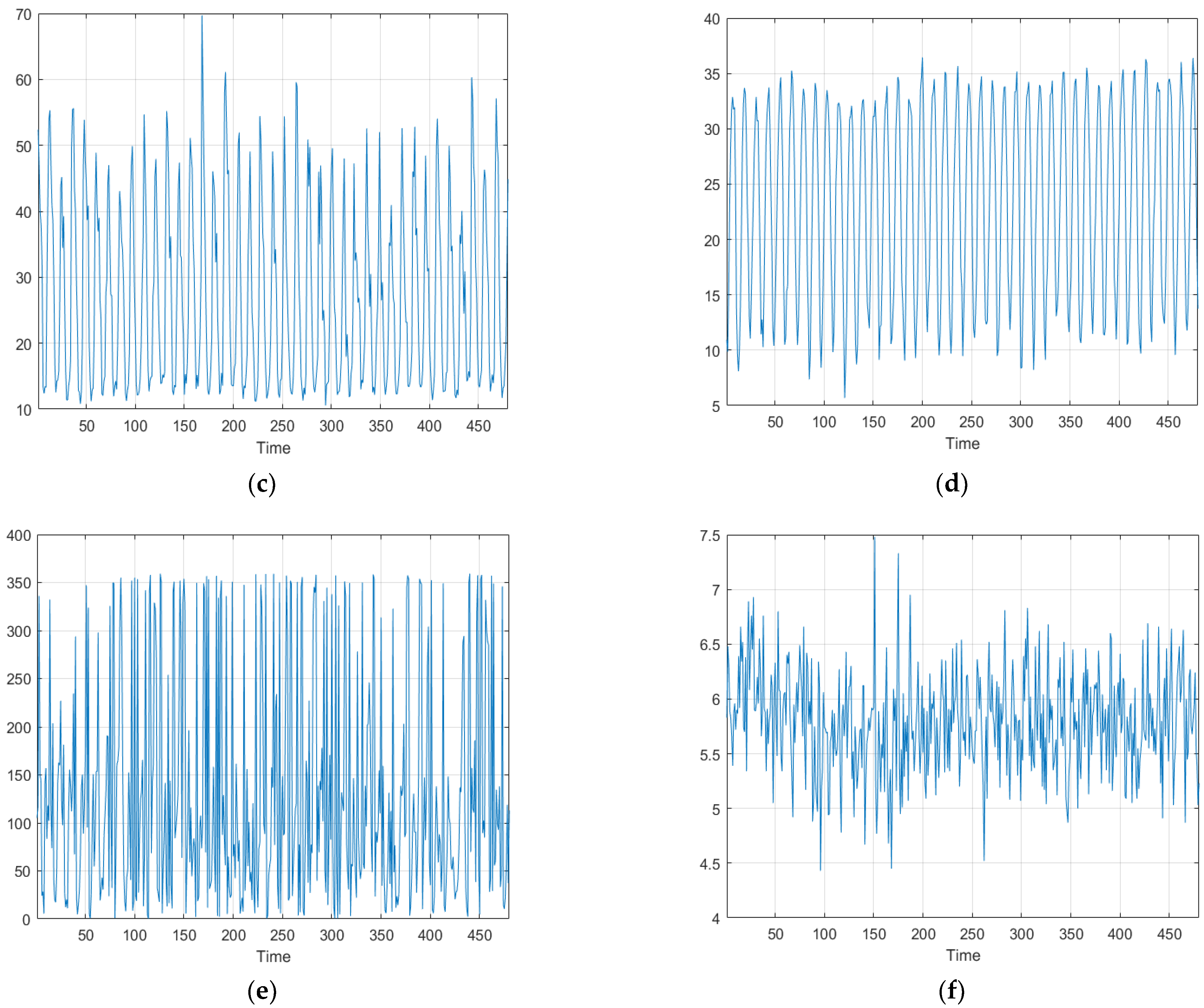
4.1. Data

The analyzed time series in this article are the geopolitical risk index (GPRAS), the total precipitation (PRECTOT), the relative humidity (RH2M), the temperature (T2M), the wind direction (WD50M), and the wind speed (WS50M). The geopolitical risk index is downloaded from https://www.matteoiacoviello.com/gpr.htm (accessed on 13 November 2021), whereas all climatic time series are downloaded from https://power.larc.nasa.gov/data-access-viewer/ (accessed on 13 November 2021). The sample spans from January 1982 to December 2021 with a monthly frequency and a total of 480 observations. Details on the data, symbols, and indices are presented in

Table 2. Brief description of studied time series.

Index	Symbol	Description
Geopolitical risk index	GPRAS	Reflects automated text-search results of the electronic archives of The New York Times, Chicago Tribune, and The Washington Post newspapers.
Total precipitation	PRECTOT	The total precipitation in mm per day.
The relative humidity	RH2M	The relative humidity measured at two meters is given in percentage.
The temperature	T2M	The temperature was measured at two meters.
The wind direction	WD50M	The wind direction was measured at 50 m in degree.
The wind speed	WS50M	The wind speed is measured at 50 m in meters per second.

. We show in

Table 3. Summary statistics.

	GPRAS	PRECTOT	RH2M	T2M	WD50M	WS50M
Mean	0.224	0.110	27.218	23.261	130.328	5.789
Median	0.150	0.000	23.815	24.455	88.940	5.800
Min	0.010	0.000	10.560	5.690	0.250	4.430
Max	3.420	3.040	69.690	36.440	359.250	7.480
Std.Dev.	0.306	0.253	13.796	8.603	117.318	0.459
Skewness	52.134	43.783	2.172	1.581	2.395	3.275
Kurtosis	6.099	5.006	0.604	−0.190	0.893	0.069
JB test	5.126 × 104 (0.000)	3.527 × 104 (0.000)	42.952 (0.001)	43.160 (0.001)	71.148 (0.001)	1.911 (0.355)
ADF test	−7.515 (0.001)	−16.856 (0.001)	−3.426 (0.001)	−2.070 (0.037)	−11.086 (0.001)	−1.120 (0.241)

Note: The value between parentheses is the associated p-value for JB and ADF tests.

some summary statistics of the studied time series which are illustrated in Figure 1.

According to Table 3, the GPRAS index is characterized by positive mean, skewness, and kurtosis coefficients and a low standard deviation. In addition, the difference between mean and maximum values reveals that there are some spikes in the GPRAS index due to geopolitical events. On the other hand, the Jarque–Bera (JB) test reveals that the distribution of the GPRAS index is not normal, whereas the augmented Dickey–Fuller (ADF) test proves that GPRAS is stationary. However, all climatic time series are characterized by positive mean, skewness, kurtosis coefficients and a high standard deviation value. Furthermore, the result of the JB test shows that PRECTOT, RH2M, T2M, and WD50M time series are not normally distributed assuming that the associated p-values are less than 5%, while the WS50M time series is normally distributed assuming that the associated p-value is greater than 5%, indicating no rejection of the initial hypothesis that the data is normally distributed. The result of the ADF test shows that PRECTOT, RH2M, T2M, and WD50M time series are stationary where the associated p-values are less than 5%. In comparison, the WS50M time series is not stationary since the associated p-value is greater than 5%, which implies no rejection of the initial hypothesis that the time series is not stationary.

Since the GPRAS index exhibits non-normal distribution and non-stationarity according to the JB test and ADF test, respectively, it is important to note that the transfer entropy method does not rely on the normality and stationarity assumptions of the variables. This method is known for its robustness in handling non-normal and non-stationary data [65,66,67], making it suitable for analyzing the GPRAS index despite its non-standard characteristics. Furthermore, it is worth mentioning that the climatic time series of PRECTOT, RH2M, T2M, WD50M, and WS50M also demonstrate non-normal distribution and, in some cases, non-stationarity. However, the analysis methodology utilized in this study is well-established for handling such data characteristics, ensuring reliable insights into the causal relationships between the geopolitical risk index and the climate change variables.

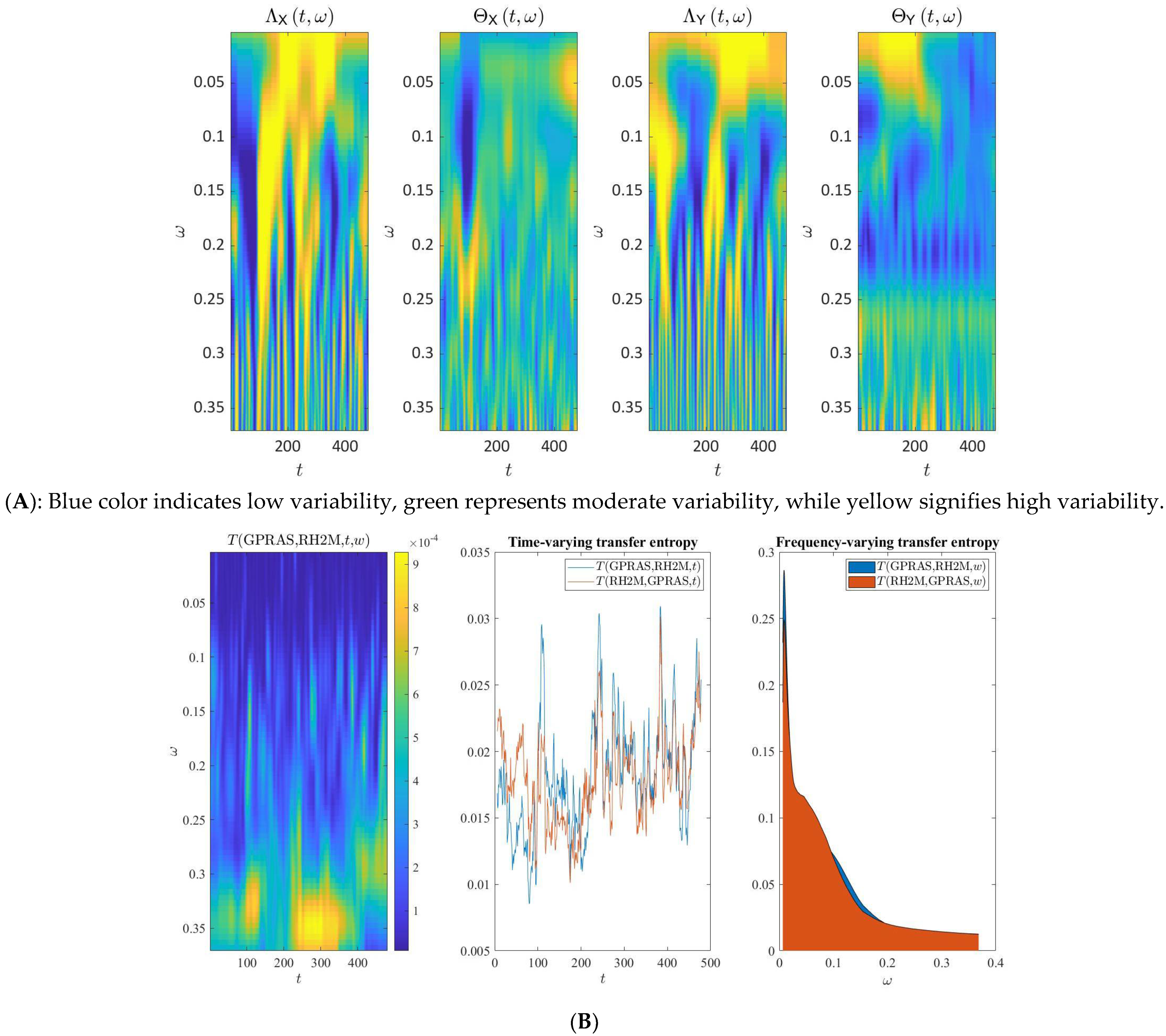
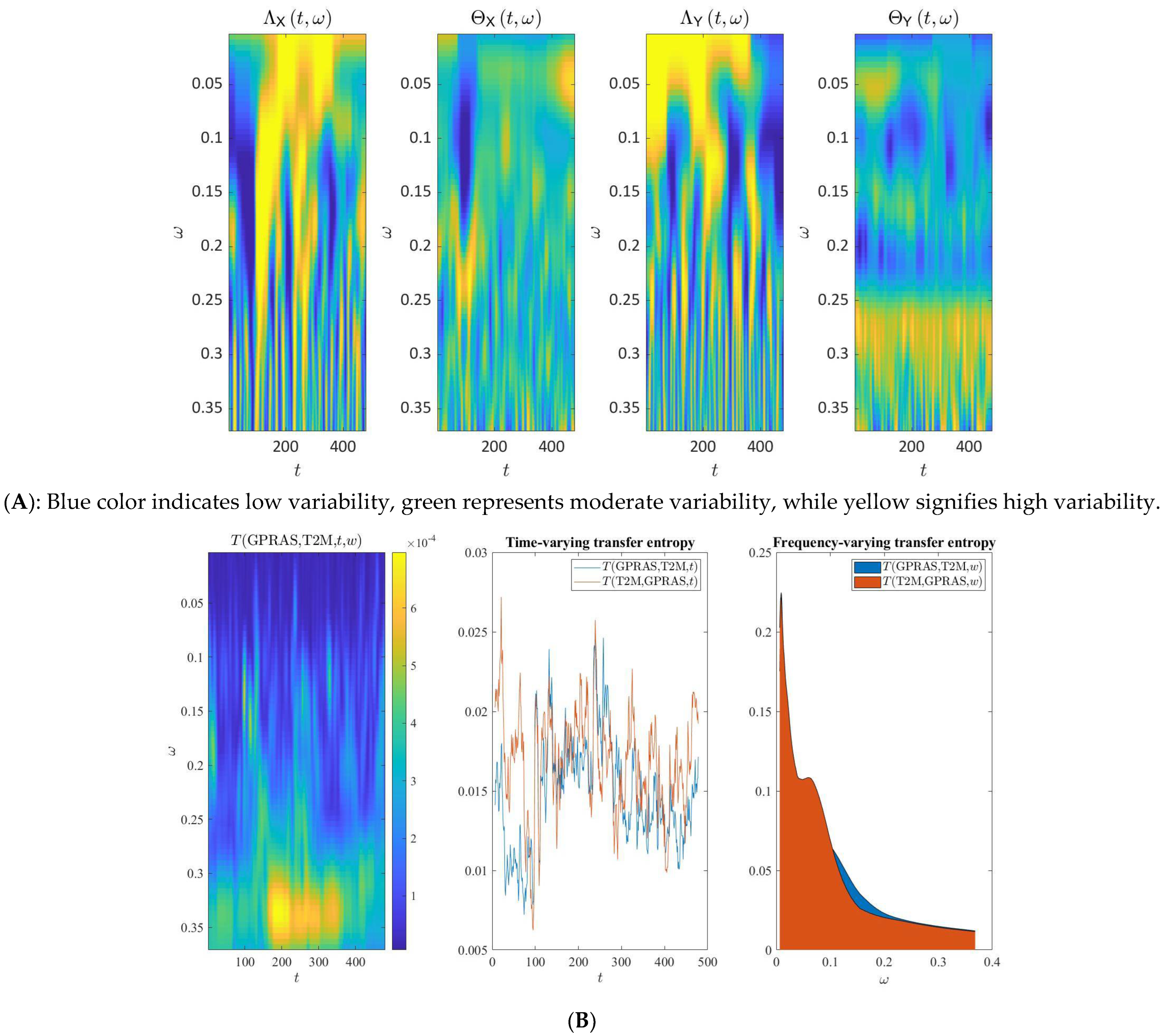
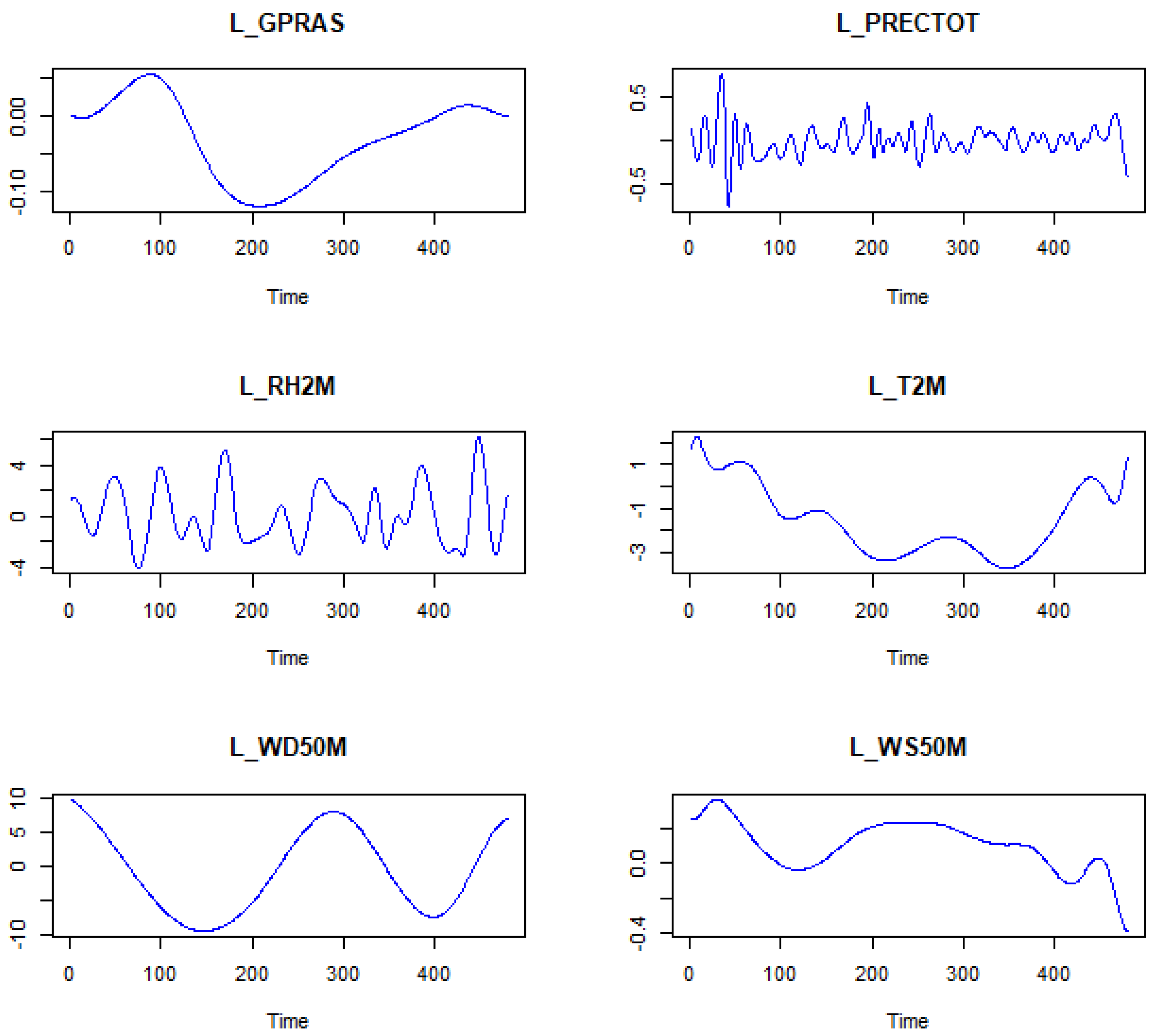
4.2. Empirical Results

The results of the causality test, using the Fourier-domain transfer entropy spectrum method, for pairs (GPRAS, PRECTOT), (GPRAS, RH2M), (GPRAS, T2M), (GPRAS, WD50M), and (GPRAS, WS50M) are illustrated in Figure 2, Figure 3, Figure 4, Figure 5 and Figure 6. For comparison between coarse-grained and fine-grained symbols, high and low values of time symbolization $\alpha$ and frequency symbolization $\beta$ are tested. Accordingly, our study chose $\alpha =\beta =3$, where the results of the used grained symbolizations are given at the top of Figure 2, Figure 3, Figure 4, Figure 5 and Figure 6. Additionally, based on the Akaike information criteria, we choose 5 as the time-lag L.

According to Figure 2B (on the left), for time interval [250,350], the information flow between GPRAS and PRECTOT indices is around 0.8 × 10⁻³ when the frequency w is around 0.35. Additionally, for time interval [150,250], the information flow between GPRAS and PRECTOT indices is around 0.5 × 10⁻³ when the w in the interval is [0.3,0.35]. When the frequency w is less than 0.15, the flow of information between GPRAS and PRECTOT indices is zero. Accordingly, we conclude that there is, in the long term, a bidirectional causality relationship running from the GPRAS index to the PRECTOT time series and conversely. Figure 2B (in the middle) shows that the bidirectional information flow is time-varying. Additionally, there is a similar behavior between bidirectional flows of information in all studied periods except the first 100 months (from January 1982 to May 1990), where the information flow from the PRECTOT time series to the GPRAS index is greater than the information flow from the GPRAS index to the PRECTOT time series.

According to Figure 2B (on the left), we remark a similar behavior of the bidirectional flow of information for all frequency intervals. Additionally, the flow of information decreases when the frequency w increases, implying that there is an information flow between these pairs of time series in the long term; however, in the short term, the information flow is zero. Based on Figure 3B (in the left), the information flow between GPRAS and RH2M indices is around 0.9 × 10⁻³ when the frequency w is around 0.35 and when the time is between 250 and 350. On the other hand, when the frequency w is less than 0.15, there is no flow of information between GPRAS and RH2M. Accordingly, we conclude that there is a bidirectional causality relationship between GPRAS and RH2M time series in the long term.

Figure 3B (in the middle) shows a global variation in bidirectional information flows over time and a similar behavior of such flows of information in all studied periods. Additionally, according to Figure 3B (on the left), we note a similar information flow for all frequencies. Furthermore, the information flow decreases when the frequency increases, implying that bidirectional causality relationships exist between these pairs of time series in the long term. However, in the short term, the information flow is zero.

From Figure 4B (on the left), the information flow between GPRAS and T2M indices is almost equal to 0.7 × 10⁻³ when the frequency w is around 0.35 and when the time is between 150 and 350. When the frequency is less than 0.15, there is no flow of information. Consequently, we conclude that there is a bidirectional causality relationship between GPRAS and T2M in the long term. Figure 4B (in the middle) shows that the bidirectional information flows are time-varying for all studied periods. According to Figure 4B (on the left), we remark a similar behavior of bidirectional information flows in all frequency intervals. Additionally, the information flow decreases when the frequency w increases, which implies a bidirectional causality relationship between these pairs of time series in the long term. However, in the short term, the information flow is zero.

Based on Figure 5B (in the left), the information flow between the GPRAS and WD50M indices is almost equal to 0.7 × 10⁻³ when the frequency w is around 0.35 for a period of [150,200]. Additionally, the flow of information between these pairs is almost equal to 0.6 × 10⁻³ when the frequency w is around 0.3 for time intervals [350,450]. When the frequency w is less than 0.15, there is no flow of information. Therefore, we conclude that there is a bidirectional causality relationship between GPRAS and WD50M time series in the medium and long terms. Figure 5B (in the middle) shows that the information flow is time-varying for all studied periods. According to Figure 5B (in the left), the information flow decreases slowly when the frequency w increases, which implies that there are bidirectional causality relationships between these pairs of time series in the medium and long terms; however, in the short term, no causality relationships are used where the information flow is zero.

According to Figure 6B (in the left), the information flow between the GPRAS and WS50M indices is almost equal to 0.6 × 10⁻³ when the frequency w is between 0.3 and 0.35 for time intervals [150,300] and [350,450]. When the frequency w is less than 0.2, there is no flow of information. Hence, we can conclude that there is a bidirectional causality relationship between the GPRAS and WS50M time series in the medium and long terms. Figure 6B (in the middle) shows that the information flow is time-varying for all studied periods. According to Figure 6B (in the left), the information flow decreases slowly when the frequency w increases, which implies that there is a bidirectional causality relationship between these pairs of time series in medium and long terms; however, in the short term, the information flow is zero, which indicates no causality relationship between such indices.

5. Robustness Check

In this section, we conduct a robustness check for the obtained results. For this goal, a variable-lag relative transfer entropy (VLRTE) causality test [13] with the empirical mode decomposition (EMD) method is used. Consider two-time series, X and Y; each time series is decomposed, with the EMD method, into intrinsic mode functions (IMFs) and a residual vector, R. These IMFs are then categorized into two terms using the fine-to-coarse approach: the short-term scale, H, and the medium-term scale, L. The residual part, R, obtained directly through the EMD method, represents the long-term scale for each time series. As a result, for time series X, we have three distinct components: H_X, L_X, and R_X, while for time series Y, the components are H_Y, L_Y, and R_Y. The empirical mode decomposition variable-lag relative transfer entropy (EMD-VL relative transfer entropy) is determined as the variable-lag relative transfer entropy, calculated between the short-term, medium-term, and long-term scales. We should note that relative transfer entropy quantifies the proportion of information flow from one time series to another.

Table 4. Variance contributions for different time scales.

Time Series	Variance as a Percentage of Original Time Series			Main Scales
	H	L	R
GPRAS	89.306	2.585	8.107	Short-term; long-term
PRECTOT	61.210	29.520	9.269	Short-term; medium-term; long-term
RH2M	1.858	83.956	14.184	Medium-term; long-term
T2M	3.314	92.95	3.735	Medium-term
WD50M	99.729	0.255	0.014	Short-term
WS50M	85.282	8.838	5.878	Short-term; medium-term; long-term

presents the distinct contributions of various time scales to their cumulative sums, allowing us to identify the principal time scales. The obtained scales are illustrated in Figure 7, Figure 8 and Figure 9.

Additionally,

Table 5. Variable-lag relative transfer entropy between different scales.

	Percentage of Information Flows
Pairs of Time Series	Short-Term Scale	Medium-Term Scale	Long-Term Scale
GPRAS → PRECTOT	0.222	0.346	0.029
PRECTOT → GPRAS	0.556	0.376	0.033
GPRAS → RH2M	5.268	0.087	2.378
RH2M → GPRAS	4.502	0.436	0.657
GPRAS → T2M	0.382	0.042	0.014
T2M → GPRAS	0.542	0.028	0.028
GPRAS → WD50M	4.121	0.066	0.028
WD50M → GPRAS	5.009	0.066	0.028
GPRAS → WS50M	0.454	0.065	1.214
WS50M → GPRAS	0.454	0.063	0.339

displays the outcomes of variable-lag relative transfer entropy for short-term, medium-term, and long-term scales.

Table 5 presents the percentage of information flow within different time scales. In the short-term scale, the information flow from GPRAS to PRECTOT is 0.222, while from PRECTOT to GPRAS, it is 0.556. These values change to 0.346 and 0.376 on the medium-term scale, respectively. These findings confirm the bidirectional causality relationships identified through the transfer entropy Fourier spectrum analysis. Additionally, on the short-term scale, the information flow from GPRAS to RH2M is 5.268, and from RH2M to GPRAS, it is 4.502. For the medium-term scale, the values are 0.436 (RH2M to GPRAS) and 0.657 (GPRAS to RH2M). These results align with the outcomes from transfer entropy in the Fourier domain, indicating a bidirectional causality between the GPRAS and RH2M time series. Furthermore, examining the relationship between GPRAS and T2M, the information flow percentages are 0.382 (GPRAS to T2M) and 0.542 (T2M to GPRAS) in the short-term scale, supporting a bidirectional causality connection, consistent with the findings from transfer entropy analysis in the Fourier domain. Shifting focus to WD50M and WS50M, the information flow percentages between GPRAS and WD50M are 4.121 (GPRAS to WD50M) and 5.009 (WD50M to GPRAS) on the short-term scale. In contrast, for WS50M, the percentage of information flow is 0.454 on the short-term scale and 1.214 on the long-term scale from GPRAS to WS50M. Notably, the information flow from WS50M to GPRAS remains at 0.454 on the short-term scale. These outcomes underscore the bidirectional causality relationships revealed by transfer entropy analysis in the Fourier domain between GPRAS and WD50M, as well as WS50M.

6. Discussion

Our study sheds light on the intricate relationships between temperature, precipitation, humidity, wind speed, wind direction, and the geopolitical risk index in Saudi Arabia. We have found compelling evidence that fluctuations in these climatic variables can influence the geopolitical risk index, and conversely, the geopolitical risk index can impact these five climatic variables.

Geopolitical risks play a significant role in amplifying climate threats through various mechanisms. Firstly, conflicts among nations can impede international cooperation on environmental issues and hinder effective climate change mitigation efforts [68]. Such hostilities and tensions may decrease the likelihood of joint climate action and increase uncertainties. Secondly, a financial link exists between geopolitical risk and climate risk, with geopolitical developments causing uncertainty in financial markets [69,70]. This financial uncertainty can impede climate action, as the financial sector is vital in supporting climate initiatives [71]. Moreover, regions with high geopolitical risks often possess abundant energy resources, establishing a third link between geopolitical risk and climate risk [48].

Furthermore, geopolitical risks can indirectly influence climate change by impacting global economic activity and international cooperation on climate change mitigation and adaptation efforts. For example, [72] suggests that geopolitical risk is a driving force for the climate change index, with green bond and clean energy markets inversely correlated with geopolitical risk at certain quantiles [56]. Reveal that geopolitical risk leads to increased CO₂ emissions, with a 1% increase in geopolitical risk resulting in a 13% rise in CO₂ emissions. Geopolitical risk indicates that the likelihood of political instability and conflicts across different regions influences business and economic activity [55]. High geopolitical risks can hinder business activity and spending, potentially slowing the adoption of low-carbon technologies and impeding the transition to sustainability. Additionally, geopolitical conflicts, such as military engagements, can directly impact the environment and exacerbate climate change. Wars, for example, release substantial greenhouse gases from burning buildings and infrastructure, disrupting agricultural and industrial activities. Although geopolitical risk does not directly impact climate change, its indirect influence on mitigation and adaptation efforts can have significant environmental and social consequences.

Conversely, increasing climate-related risks and activities can lead to geopolitical problems or crises. The shift from fossil fuels to renewable energy presents challenges and opportunities in addressing climate risk [73]. Nations may compete for benefits during this transition, and some experts argue that the rapidly expanding renewable energy industry could introduce a new type of geopolitical risk [74]. Resource scarcity, such as land for renewable energy development, can heighten geopolitical tensions among nations. For instance, the Danube River flows through five nations outside the European Union and nine countries within it, resulting in geopolitical tensions due to economic assistance and access to European Union privileges.

Moreover, climate change’s increased frequency and intensity of extreme weather events significantly affect the geopolitical risk index. Floods, droughts, hurricanes, and other extreme climate conditions can cause substantial damage to buildings, disrupt logistical systems, and harm economic growth. These events may also lead to social and political unrest, especially in countries facing political and economic instability.

Climate change poses a formidable threat to crucial resources such as water, food, and energy [75]. Rising temperatures and variable rainfall can result in water scarcity, crop failures, and reduced agricultural productivity, leading to food insecurity, increased living costs, and social and political tensions. Moreover, climate-induced competition for scarce resources among nations can exacerbate and create new geopolitical tensions. Additionally, the migration of people due to climate change can contribute to social and political tensions, particularly in countries unwilling to accept large numbers of refugees [76,77,78]. Given climate change’s significant and widespread effects on the geopolitical risk index, a coordinated and integrated approach from policymakers, scientists, and civil society is crucial in mitigating the risks associated with geopolitics and environmental change.

Overall, our study underscores the complex interplay between climate variables and geopolitical risk in Saudi Arabia. It emphasizes the need for a comprehensive approach to address the challenges of climate change and its implications for geopolitical dynamics.

7. Conclusions

Using the Fourier-domain transfer entropy method, the present study examined the relationship between geopolitical risk and climate change in Saudi Arabia from January 1982 to December 2021. Our results indicate a strong bidirectional causality between the five climatic indicators and the geopolitical risk index. These findings have important implications for policymakers, shareholders, and financial managers. Leaders must focus on reducing greenhouse gas emissions and mitigating rising temperatures to address the interconnected challenges of geopolitical risk and climate change. Climate change significantly impacts geopolitical risk worldwide, increasing costs due to rising temperatures and frequent extreme weather events. To improve the well-being and future of people, some countries’ finances must be allocated to environmental development. Policymakers should take innovative fiscal and monetary measures to encourage businesses to adopt environmentally friendly practices. Incentives should be provided to boost the economy and promote clean manufacturing and ecological fabrication services, which can help reduce harmful gas emissions and minimize environmental damage.

Additionally, geopolitical conflicts and the concurrent rush to find new energy supplies highlight the importance of energy security, which significantly impacts climate change through the transition to renewable energy. Furthermore, shareholders and financial managers should manage their portfolios by incorporating geopolitical risk, renewable energy, green bonds, and climate change as environmentally friendly assets. As several recent studies have indicated, future research may re-evaluate the accountability of carbon reserves [79]. This could prove useful in evaluating climate change and carbon emissions strategies.

In forthcoming research, investigators have an intriguing opportunity to delve deeper into the dynamics underpinning the observed patterns within the studied time series. A prospective avenue involves the implementation of the robust correlation dimension estimator proposed by [80], utilizing the Gaussian kernel correlation integral [81]. This innovative approach promises a meticulous exploration into whether the examined time series might manifest chaotic behavior. Should the findings point to chaos, a captivating prospect emerges: developing a specialized dynamical chaotic process tailored to model the intricate interactions intrinsic to these time series. Such a foray into chaotic dynamics offers the potential to unearth novel insights into the underlying mechanisms that govern the observed phenomena, thereby paving the way toward a more profound comprehension and potential breakthroughs in this dynamic field.

In parallel explorations, researchers may contemplate harnessing intraday data to comprehensively delineate the trajectory of the Russian invasion of Ukraine, augmenting their insights through high-frequency data on volatility. To refine estimations, prospective inquiries could integrate quantile the cross-spectral techniques pioneered in [82] and the Markov-switching dependence methodologies advanced by [79], thereby shedding greater light on the nuanced actions of assets. Furthermore, the prospective utilization of the time-varying parameter vector autoregressive model, as demonstrated by [83], might prove valuable in assessing the impact of green finance on the environmental protection index.

References

1. World Bank. World Development Indicators. 2010. Available online: https://data.worldbank.org (accessed on 1 June 2023).
2. UN-Habitat. Annual Report 2010; United Nations: New York, NY, USA, 2010; ISBN 978-92-1-132336-8. Available online: https://unhabitat.org/annual-report-2021 (accessed on 1 June 2023).
3. Michel, D.; Klimes, M.; Eriksson, M. Climate Change and (In)Security in Transboundary River Basins. In Handbook of Security and the Environment; Edward Elgar: Northampton, MA, USA, 2021; pp. 62–75. [Google Scholar]
4. Alrashed, F.; Asif, M. Climatic Classifications of Saudi Arabia for Building Energy Modelling. Energy Procedia 2015, 75, 1425–1430. [Google Scholar] [CrossRef]
5. Al-Maamary, H.M.S.; Kazem, H.A.; Chaichan, M.T. Climate Change: The Game Changer in the Gulf Cooperation Council Region. Renew. Sustain. Energy Rev. 2017, 76, 555–576. [Google Scholar] [CrossRef]
6. Tolba, M.K.; Saab, N.W. Arab environment: Climate change. In 2009 Report of The Arab Forum for Environment and Development; Tolba, M.K., Saab, N.W., Eds.; AFED: Beirut, Lebanon, 2009; Available online: http://www.afedonline.org/afedreport09/Full%20English%20Report.pdf (accessed on 7 April 2019).
7. Azamathulla, H.; Rathnayake, U.; Shatnawi, A. Gene Expression Programming and Artificial Neural Network to Estimate Atmospheric Temperature in Tabuk, Saudi Arabia. Appl. Water Sci. 2018, 8, 184. [Google Scholar] [CrossRef]
8. Nassar, M.; Bakr, R.; Abdeldayem, M.; El-Barky, N.; Kotb, T. Seasonal Abundance of Mosquitoes in Jizan Province. Egypt. Acad. J. Biol. Sci. Entomol. 2016, 9, 1–13. [Google Scholar] [CrossRef]
9. Lee, C.-C.; Olasehinde-Williams, G.; Akadiri, S.S. Geopolitical Risk and Tourism: Evidence from Dynamic Heterogeneous Panel Models. Int. J. Tour. Res. 2021, 23, 26–38. [Google Scholar] [CrossRef]
10. Caldara, D.; Iacoviello, M. Measuring Geopolitical Risk. Am. Econ. Rev. 2022, 112, 1194–1225. [Google Scholar] [CrossRef]
11. Olasehinde-Williams, G.O.; Balcilar, M. The Effect of Geopolitical Risks on Insurance Premiums. J. Public Aff. 2022, 22, e2387. [Google Scholar] [CrossRef]
12. Li, B.; Chang, C.-P.; Chu, Y.; Sui, B. Oil Prices and Geopolitical Risks: What Implications are Offered via Multi-Domain Investigations? Energy Environ. 2020, 31, 492–516. [Google Scholar] [CrossRef]
13. Dhifaoui, Z.; Khalfaoui, R.; Abedin, M.Z.; Shi, B. Quantifying Information Transfer Among Clean Energy, Carbon, Oil, and Precious Metals: A Novel Transfer Entropy-Based Approach. Financ. Res. Lett. 2022, 49, 103138. [Google Scholar] [CrossRef]
14. Dhifaoui, Z.; Khalfaoui, R.; Jabeur, S.B.; Abedin, M.Z. Exploring the Effect of Climate Risk on Agricultural and Food Stock Prices: Fresh Evidence from EMD-Based Variable-Lag Transfer Entropy Analysis. J. Environ. Manag. 2023, 326, 116789. [Google Scholar] [CrossRef]
15. Dibiasi, A.; Abberger, K.; Siegenthaler, M.; Sturm, J.-E. The Effects of Policy Uncertainty on Investment: Evidence from the Unexpected Acceptance of a Far-Reaching Referendum in Switzerland. Eur. Econ. Rev. 2018, 104, 38–67. [Google Scholar] [CrossRef]
16. Xue, C.; Shahbaz, M.; Ahmed, Z.; Ahmad, M.; Sinha, A. Clean Energy Consumption, Economic Growth, and Environmental Sustainability: What is the Role of Economic Policy Uncertainty? Renew. Energy 2022, 184, 899–907. [Google Scholar] [CrossRef]
17. Yu, M.; Wang, N. The Influence of Geopolitical Risk on International Direct Investment and Its Counter-Measures. Sustainability 2023, 15, 2522. [Google Scholar] [CrossRef]
18. Eksi, O.; Tas, B.K.O. Time-Varying Effect of Uncertainty Shocks on Unemployment. Econ. Model. 2022, 110, 105810. [Google Scholar] [CrossRef]
19. Azad, N.F.; Serletis, A. Spillovers of U.S. Monetary Policy Uncertainty on Inflation-Targeting Emerging Economies. Emerg. Mark. Rev. 2021, 51, 100875. [Google Scholar] [CrossRef]
20. Haque, Q.; Magnusson, L.M. Uncertainty Shocks and Inflation Dynamics in the U.S. Econ. Lett. 2021, 202, 109825. [Google Scholar] [CrossRef]
21. Chiang, T.C. The Effects of Economic Uncertainty, Geopolitical Risk, and Pandemic Upheaval on Gold Prices. Resour. Policy 2022, 76, 102546. [Google Scholar] [CrossRef]
22. Jiao, Y.; Xiao, X.; Bao, X. Economic Policy Uncertainty, Geopolitical Risks, Energy Output, and Ecological Footprint: Empirical Evidence from China. Energy Rep. 2022, 8, 324–334. [Google Scholar] [CrossRef]
23. Gupta, R.; Gozgor, G.; Kaya, H.; Demir, E. Effects of Geopolitical Risks on Trade Flows: Evidence from the Gravity Model. Eurasian Econ. Rev. 2019, 9, 515–530. [Google Scholar] [CrossRef]
24. Li, Y.; Huang, J.; Chen, J. Dynamic Spillovers of Geopolitical Risks and Gold Prices: New Evidence from 18 Emerging Economies. Resour. Policy 2021, 70, 101938. [Google Scholar] [CrossRef]
25. Li, Y.; Huang, J.; Gao, W.; Zhang, H. Analyzing the Time-Frequency Connectedness Among Oil, Gold Prices, and BRICS Geopolitical Risks. Resour. Policy 2021, 73, 102134. [Google Scholar] [CrossRef]
26. Su, C.-W.; Khan, K.; Tao, R.; Nicoleta-Claudia, M. Does Geopolitical Risk Strengthen or Depress Oil Prices and Financial Liquidity? Evidence from Saudi Arabia. Energy 2019, 187, 116003. [Google Scholar] [CrossRef]
27. Kannadhasan, M.; Das, D. Do Asian Emerging Stock Markets React to International Economic Policy Uncertainty and Geopolitical Risk Alike? A Quantile Regression Approach. Financ. Res. Lett. 2020, 34, 101276. [Google Scholar] [CrossRef]
28. Hoque, M.E.; Zaidi, M.A.S. Global and Country-Specific Geopolitical Risk Uncertainty and Stock Return of Fragile Emerging Economies. Borsa Istanb. Rev. 2020, 20, 197–213. [Google Scholar] [CrossRef]
29. Yang, K.; Wei, Y.; Li, S.; He, J. Geopolitical Risk and Renewable Energy Stock Markets: An Insight from Multiscale Dynamic Risk Spillover. J. Clean. Prod. 2021, 279, 123429. [Google Scholar] [CrossRef]
30. Smales, L.A. Geopolitical Risk and Volatility Spillovers in Oil and Stock Markets. Q. Rev. Econ. Financ. 2021, 80, 358–366. [Google Scholar] [CrossRef]
31. Sohag, K.; Hammoudeh, S.; Elsayed, A.H.; Mariev, O.; Safonova, Y. Do Geopolitical Events Transmit Opportunity or Threat to Green Markets? Decomposed Measures of Geopolitical Risks. Energy Econ. 2022, 111, 106068. [Google Scholar] [CrossRef]
32. Flouros, F.; Pistikou, V.; Plakandaras, V. Geopolitical Risk as a Determinant of Renewable Energy Investments. Energies 2022, 15, 1498. [Google Scholar] [CrossRef]
33. Li, S.; Tu, D.; Zeng, Y.; Gong, C.; Yuan, D. Does Geopolitical Risk Matter in Crude Oil and Stock Markets? Evidence from Disaggregated Data. Energy Econ. 2022, 113, 106191. [Google Scholar] [CrossRef]
34. Gong, X.; Xu, J. Geopolitical Risk and Dynamic Connectedness Between Commodity Markets. Energy Econ. 2022, 110, 106028. [Google Scholar] [CrossRef]
35. Umar, M.; Riaz, Y.; Yousaf, I. Impact of Russian-Ukraine War on Clean Energy, Conventional Energy, and Metal Markets: Evidence from Event Study Approach. Resour. Policy 2022, 79, 102966. [Google Scholar] [CrossRef]
36. Steffen, B.; Patt, A. A Historical Turning Point? Early Evidence on How the Russia-Ukraine War Changes Public Support for Clean Energy Policies. Energy Res. Soc. Sci. 2022, 91, 102758. [Google Scholar] [CrossRef]
37. Oloko, T.; Olaniran, A.; Lasisi, L. Hedging Global and Country-Specific Geopolitical Risks with South Korean Stocks: A Predictability Approach. Asian Econ. Lett. 2021, 2, 24418. [Google Scholar] [CrossRef]
38. Bilgin, M.H.; Gozgor, G.; Karabulut, G. How Do Geopolitical Risks Affect Government Investment? An Empirical Investigation. Def. Peace Econ. 2020, 31, 550–564. [Google Scholar] [CrossRef]
39. Zhang, Z.; He, M.; Zhang, Y.; Wang, Y. Geopolitical Risk Trends and Crude Oil Price Predictability. Energy 2022, 258, 124824. [Google Scholar] [CrossRef]
40. Cai, Y.; Wu, Y. Time-Varying Interactions between Geopolitical Risks and Renewable Energy Consumption. In ADBI Working Paper; Asian Development Bank Institute: Tokyo, Japan, 2020; p. 1089. Available online: https://www.adb.org/publications/time-varyinginteractionsbetween-geopolitical-risks-renewable-energy-consumption (accessed on 1 June 2023).
41. Sweidan, O.D. The Geopolitical Risk Effect on US Renewable Energy Deployment. J. Clean. Prod. 2021, 293, 126189. [Google Scholar] [CrossRef]
42. Demiralay, S.; Kilincarslan, E. The Impact of Geopolitical Risks on Travel and Leisure Stocks. Tour. Manag. 2019, 75, 460–476. [Google Scholar] [CrossRef]
43. Cheng, C.H.J.; Chiu, C.-W.J. How Important Are Global Geopolitical Risks to Emerging Countries? Int. Econ. 2018, 156, 305–325. [Google Scholar] [CrossRef]
44. Zhao, W.; Zhong, R.; Sohail, S.; Majeed, M.; Ullah, S. Geopolitical Risks, Energy Consumption, and CO2 Emissions in BRICS: An Asymmetric Analysis. Environ. Sci. Pollut. Res. 2021, 28, 39668–39679. [Google Scholar] [CrossRef]
45. Anasori, E.; Kucukergin, K.G.; Soliman, M.; Tulucu, F.; Altinay, L. How Can the Subjective Well-being of Nurses Be Predicted? Understanding the Mediating Effect of Psychological Distress, Psychological Resilience, and Emotional Exhaustion. J. Serv. Theory Pract. 2022, 32, 762–780. [Google Scholar] [CrossRef]
46. Goes, C.; Bekkers, E. The Impact of Geopolitical Conflicts on Trade, Growth, and Innovation: An Illustrative Simulation Study. Available online: https://cepr.org/voxeu/columns/impact-geopolitical-conflicts-trade-growth-and-innovation-illustrative-simulation (accessed on 1 June 2023).
47. Sowby, R.B.; Capener, A. The Influence of Precipitation on the Energy Footprint of Denver’s Water Supply: A 20-year Analysis and Implications for Climate Change. Energy Nexus 2023, 9, 100166. [Google Scholar] [CrossRef]
48. Jin, Y.; Zhao, H.; Bu, L.; Zhang, D. Geopolitical Risk, Climate Risk, and Energy Markets: A Dynamic Spillover Analysis. Int. Rev. Financ. Anal. 2023, 87, 102597. [Google Scholar] [CrossRef]
49. Shen, L.; Hong, Y. Can Geopolitical Risks Excite Germany Economic Policy Uncertainty: Rethinking in the Context of the Russia-Ukraine Conflict. Financ. Res. Lett. 2023, 51, 103420. [Google Scholar] [CrossRef]
50. Soltani, H.; Triki, M.; Ghandri, M.; Abderzag, F. Does Geopolitical Risk and Financial Development Matter for Economic Growth in MENA Countries? J. Int. Stud. 2021, 14, 103–116. [Google Scholar] [CrossRef]
51. Le, A.-T.; Tran, T.P. Does Geopolitical Risk Matter for Corporate Investment? Evidence from Emerging Countries in Asia. J. Multinatl. Financ. Manag. 2021, 62, 100703. [Google Scholar] [CrossRef]
52. Hailemariam, A.; Ivanovski, K. The Impact of Geopolitical Risk on Tourism. Curr. Issues Tour. 2021, 24, 3134–3140. [Google Scholar] [CrossRef]
53. Alsagr, N.; Almazor, S.F.V.H. Oil Rent, Geopolitical Risk, and Banking Sector Performance. Int. J. Energy Econ. Policy 2020, 10, 305–314. [Google Scholar] [CrossRef]
54. Olanipekun, I.O.; Alola, A.A. Crude Oil Production in the Persian Gulf amidst Geopolitical Risk, Cost of Damage, and Resources Rents: Is There Asymmetric Inference? Resour. Policy 2020, 69, 101873. [Google Scholar] [CrossRef]
55. Akadiri, S.S.; Eluwole, K.K.; Akadiri, A.C.; Avci, T. Does Causality between Geopolitical Risk, Tourism, and Economic Growth Matter? Evidence from Turkey. J. Hosp. Tour. Manag. 2020, 43, 273–277. [Google Scholar] [CrossRef]
56. Anser, M.K.; Syed, Q.R.; Apergis, N. Does Geopolitical Risk Escalate CO2 Emissions? Evidence from the BRICS Countries. Environ. Sci. Pollut. Res. 2021, 28, 48011–48021. [Google Scholar] [CrossRef]
57. Anser, M.K.; Syed, Q.R.; Lean, H.H.; Alola, A.A.; Ahmad, M. Do Economic Policy Uncertainty and Geopolitical Risk Lead to Environmental Degradation? Evidence from Emerging Economies. Sustainability 2021, 13, 5866. [Google Scholar] [CrossRef]
58. Adams, S.; Adedoyin, F.; Olaniran, E.; Bekun, F.V. Energy Consumption, Economic Policy Uncertainty, and Carbon Emissions: Causality Evidence from Resource-rich Economies. Econ. Anal. Policy 2020, 68, 179–190. [Google Scholar] [CrossRef]
59. Alsagr, N.; Hemmen, S. The Impact of Financial Development and Geopolitical Risk on Renewable Energy Consumption: Evidence from Emerging Markets. Environ. Sci. Pollut. Res. 2021, 28, 25906–25919. [Google Scholar] [CrossRef] [PubMed]
60. Mohsin Hashmi, S.; Bhowmik, R.; Inglesi-Lotz, R.; Syed, Q. Investigating the Environmental Kuznets Curve Hypothesis amidst Geopolitical Risk: Global Evidence using Bootstrap ARDL Approach. Environ. Sci. Pollut. Res. 2021, 29, 24049–24062. [Google Scholar] [CrossRef]
61. Tian, Y.; Wang, Y.; Zhang, Z.; Sun, P. Fourier-Domain Transfer Entropy Spectrum. Phys. Rev. Res. 2021, 3, L042040. [Google Scholar] [CrossRef]
62. James, R.G.; Barnett, N.; Crutchfield, J.P. Information Flows? A Critique of Transfer Entropies. Phys. Rev. Lett. 2016, 116, 1–6. [Google Scholar] [CrossRef]
63. Wyner, A.D. A Definition of Conditional Mutual Information for Arbitrary Ensembles. Inf. Control. 1978, 38, 51–59. [Google Scholar] [CrossRef]
64. Bandt, C.; Pompe, B. Permutation Entropy: A Natural Complexity Measure for Time Series. Phys. Rev. Lett. 2002, 88, 174102. [Google Scholar] [CrossRef]
65. Jafari-Mamaghani, M.; Tyrcha, J. Transfer Entropy Expressions for a Class of Non-Gaussian Distributions. Entropy 2014, 16, 1743–1755. [Google Scholar] [CrossRef]
66. Liu, A.; Chen, J.; Yang, S.Y.; Hawkes, A.G. The Flow of Information in Trading: An Entropy Approach to Market Regimes. Entropy 2020, 22, 1064. [Google Scholar] [CrossRef]
67. Papana, A.; Kyrtsou, C.; Kugiumtzis, D.; Diks, C. Detecting Causality in Non-Stationary Time Series Using Partial Symbolic Transfer Entropy: Evidence in Financial Data. Comput. Econ. 2016, 47, 341–365. [Google Scholar] [CrossRef]
68. Acheampong, A.O.; Opoku, E.E.O.; Aluko, O.A. The Roadmap to Net-zero Emission: Do Geopolitical Risk and Energy Transition Matter? J. Public Aff. 2023, e2882. [Google Scholar] [CrossRef]
69. Shabir, M.; Jiang, P.; Shahab, Y.; Wang, P. Geopolitical, Economic Uncertainty and Bank Risk: Do CEO Power and Board Strength Matter? Int. Rev. Financ. Anal. 2023, 87, 102603. [Google Scholar] [CrossRef]
70. Sharif, A.; Aloui, C.; Yarovaya, L. COVID-19 Pandemic, Oil Prices, Stock Market, Geopolitical Risk and Policy Uncertainty Nexus in the US Economy: Fresh Evidence from the Wavelet-based Approach. Int. Rev. Financ. Anal. 2020, 70, 101496. [Google Scholar] [CrossRef]
71. Long, S.; Lucey, B.; Kumar, S.; Zhang, D.; Zhang, Z. Climate Finance: What We Know and What We Should Know? J. Clim. Financ. 2022, 1, 100005. [Google Scholar] [CrossRef]
72. Simionescu, M.; Radulescu, M.; Balsalobre-Lorente, D.; Cifuentes-Faura, J. Pollution, Political Instabilities and Electricity Price in the CEE Countries During the War Time. J. Environ. Manag. 2023, 343, 118206. [Google Scholar] [CrossRef]
73. Vakulchuk, R.; Overland, I.; Scholten, D. Renewable Energy and Geopolitics: A Review. Renew. Sustain. Energy Rev. 2020, 122, 109547. [Google Scholar] [CrossRef]
74. Li, H.; Liu, Y.; Xu, B. Does Target Country’s Climate Risk Matter in Cross-border M&A? The Evidence in the Presence of Geopolitical Risk. J. Environ. Manag. 2023, 344, 118439. [Google Scholar]
75. Omar, M.E.D.M.; Moussa, A.M.A.; Hinkelmann, R. Impacts of Climate Change on Water Quantity, Water Salinity, Food Security, and Socioeconomy in Egypt. Water Sci. Eng. 2021, 14, 17–27. [Google Scholar] [CrossRef]
76. Ahmed, B. Who Takes Responsibility for the Climate Refugees? Int. J. Clim. Change Strateg. Manag. 2017, in press. [Google Scholar] [CrossRef]
77. Balsari, C.; Dresser, S.; Leaning, J. Climate Change, Migration, and Civil Strife. Curr. Environ. Health Rep. 2020, 7, 404–414. [Google Scholar] [CrossRef] [PubMed]
78. Methmann, C.; Oels, A. From “fearing” to “empowering” climate refugees: Governing climate-induced migration in the name of resilience. Secur. Dialogue 2015, 46, 51–68. [Google Scholar] [CrossRef]
79. Tiwari, A.K.; Abakah, E.J.A.; Le, T.-L.; la Hiz, D.I.L. Markov-Switching Dependence Between Artificial Intelligence and Carbon Price: The Role of Policy Uncertainty in the Era of the 4th Industrial Revolution and the Effect of COVID-19 Pandemic. Technol. Forecast. Soc. Change 2021, 163, 120434. [Google Scholar] [CrossRef]
80. Dhifaoui, Z. Robust to Noise and Outliers Estimator of Correlation Dimension. Chaos Solitons Fractals 2016, 93, 169–174. [Google Scholar] [CrossRef]
81. Dhifaoui, Z. Statistical Moments of Gaussian Kernel Correlation Sum and Weighted Least Square Estimator of Correlation Dimension and Noise Level. J. Stat. Plann. Inference 2018, 193, 55–69. [Google Scholar] [CrossRef]
82. Barunik, J.; Kley, T. Quantile Coherency: A General Measure for Dependence Between Cyclical Economic Variables. Econom. J. 2019, 22, 131–152. [Google Scholar] [CrossRef]
83. Antonakakis, N.; Chatziantoniou, I.; Gabauer, D. Refined Measures of Dynamic Connectedness Based on TVP-VAR. MPRA 2017, 78282, 1–15. [Google Scholar]
Figure 1. Studied time series: (a) GPRAS index. (b) PRECTOT time series. (c). RH2M time series. (d) T2M time series. (e) WD50M time series. (f) WS50M time series.
Sustainability 15 13579 g001aSustainability 15 13579 g001b
Figure 2. Fourier−domain transfer entropy spectrum analysis for the (GPRAS, PRECTOT) time series. (A) Grained symbolization with α = β = 3 . (B) The Fourier−domain transfer entropy spectrum (left), the time−varying transfer entropy (middle), and the frequency−varying transfer entropy (right).
Sustainability 15 13579 g002
Figure 3. Fourier−domain transfer entropy spectrum analysis for the (GPRAS, RH2M) time series. (A) Grained symbolization with α = β = 3 . (B) The Fourier−domain transfer entropy spectrum (left), the time−varying transfer entropy (middle), and the frequency−varying transfer entropy (right).
Sustainability 15 13579 g003
Figure 4. Fourier−domain transfer entropy spectrum analysis for the (GPRAS, T2M) time series. (A) Grained symbolization with α = β = 3 . (B) The Fourier−domain transfer entropy spectrum (left), the time−varying transfer entropy (middle), and the frequency−varying transfer entropy (right).
Sustainability 15 13579 g004
Figure 5. Fourier−domain transfer entropy spectrum analysis for the (GPRAS, WD50M) time series. (A) Grained symbolization with α = β = 3 . (B) The Fourier−domain transfer entropy spectrum (left), the time−varying transfer entropy (middle), and the frequency−varying transfer entropy (right).
Sustainability 15 13579 g005
Figure 6. Fourier−domain transfer entropy spectrum analysis for the (GPRAS, WS50M) time series. (A) Grained symbolization with α = β = 3 . (B) The Fourier−domain transfer entropy spectrum (left), the time−varying transfer entropy (middle), and the frequency−varying transfer entropy (right).
Sustainability 15 13579 g006
Figure 7. The short−term scale of different time series.
Sustainability 15 13579 g007
Figure 8. The medium−term scale of different time series.
Sustainability 15 13579 g008
Figure 9. The long−term scale of different time series.
Sustainability 15 13579 g009