Abstract
Current research studies offer an investigation of machine learning methods used for forecasting rainfall in urban metropolitan cities. Time series data, distinguished by their temporal complexities, are exploited using a unique data segmentation approach, providing discrete training, validation, and testing sets. Two unique models are created: Model-1, which is based on daily data, and Model-2, which is based on weekly data. A variety of performance criteria are used to rigorously analyze these models. CatBoost, XGBoost, Lasso, Ridge, Linear Regression, and LGBM are among the algorithms under consideration. This research study provides insights into their predictive abilities, revealing significant trends across the training, validation, and testing phases. The results show that ensemble-based algorithms, particularly CatBoost and XGBoost, outperform in both models. CatBoost emerged as the model of choice throughout all assessment stages, including training, validation, and testing. The MAE was 0.00077, the RMSE was 0.0010, the RMSPE was 0.49, and the R2 was 0.99, confirming CatBoost’s unrivaled ability to identify deep temporal intricacies within daily rainfall patterns. Both models had an R2 of 0.99, indicating their remarkable ability to predict weekly rainfall trends. Significant results for XGBoost included an MAE of 0.02 and an RMSE of 0.10, indicating their ability to handle longer time intervals. The predictive performance of Lasso, Ridge, and Linear Regression varies. Scatter plots demonstrate the robustness of CatBoost and XGBoost by demonstrating their capacity to sustain consistently low prediction errors across the dataset. This study emphasizes the potential to transform urban meteorology and planning, improve decision-making through precise rainfall forecasts, and contribute to disaster preparedness measures.
1. Introduction
Forecasting rainfall is an important part of weather prediction that has a big impact on multiple sectors, including agriculture, water resource management, disaster planning, and public safety [1]. For the best agricultural planning, water reservoir management, flood control measures, and early warning systems for potential natural disasters, accurate rainfall predictions are essential. The shortcomings of conventional rainfall forecasting techniques include their reliance on past trends and oversimplified mathematical models [2]. Especially during catastrophic weather events, these traditional methodologies frequently fail to adequately predict the complex and dynamic character of weather systems [3]. Inaccurate rainfall predictions can lead to considerable economic losses, failed crops, and even possible threats to human life [4]. For ages, scientists have been studying how to predict when it will rain. Early attempts to forecast rainfall relied on the observation of a variety of natural occurrences, including cloud formations and animal behavior. Weather stations were constructed as technology developed to gather and evaluate meteorological data [5]. The development of traditional forecasting approaches, such as numerical models based on physical laws and statistical methods utilizing historical data, was greatly influenced by these stations [6]. Accurate rainfall predictions are vital for managing water resources, issuing flood warnings [7], and designing resilient urban infrastructure [8]. They empower cities to prepare for disasters, minimize damage, and protect lives [9]. From resource allocation to emergency response [10], precise forecasts play a pivotal role in enhancing community resilience [11,12].
Traditional methods have been used to forecast rainfall using statistical correlations and historical data. These techniques include persistent forecasting, climatological techniques, and empirical models. In order to create predictions, empirical models employ statistical correlations between rainfall and certain meteorological data. These models frequently employ regression techniques to detect relationships between rainfall and other variables [13]. Empirical models try to determine correlations between these variables and projected rainfall by examining historical weather patterns. The empirical technique known as Multiple Linear Regression (MLR) is simple and used to predict rainfall. Based on past data, MLR forecasts future rainfall by calculating the coefficients of variables. MLR may have trouble with the complicated and non-linear interactions seen in meteorological data, even though it can capture basic correlations between variables [14,15,16]. The extension of MLR is stepwise regression. The subsets of meteorological factors that are most important for predicting rainfall are automatically chosen by this empirical technique [17,18].
Empirical approaches are essential in rainfall forecasting, especially when data and computing resources are limited. They provide rather complex forecasts compared with simpler methods such as persistence or climatological approaches and provide useful insights into the links between meteorological factors and rainfall. Empirical approaches, on the other hand, may have problems in capturing complicated non-linear relationships in meteorological data [19]. Researchers routinely combine empirical methodology with machine learning techniques to improve the accuracy and robustness of rainfall forecasts [20,21]. Machine learning has developed as a potent method for forecasting rainfall, capable of identifying complicated correlations and patterns in meteorological data. For this goal, several machine learning algorithms have been investigated, each with its own set of strengths and applications. For example, artificial neural networks (ANN) [22,23], recurrent neural networks (RNN) [24,25], random forest (RF) [26], gaussian process regression (GPR) [27], gradient-boosting [28], extreme gradient boosting [29], and long-short term memory (LSTM) [30].
Random Forest is an ensemble learning approach for improving rainfall forecasting accuracy by combining numerous decision trees [31]. This model is capable of dealing with non-linear interactions between meteorological factors and rainfall patterns [32]. Its ability to capture complicated weather patterns makes it an invaluable tool for improving overall forecast performance [33]. Support Vector Regression (SVR) is a machine learning model for regression problems that is based on Support Vector Machines (SVMs) [34,35]. SVR can capture non-linear correlations between meteorological factors and rainfall in rainfall forecasting. It seeks the hyperplane that best matches data while allowing for some inaccuracy [36]. SVR needs careful hyperparameter adjustment and can be computationally demanding for big datasets [37,38]. Time series analysis techniques based on machine learning provide a variety of potent ways to enhance rainfall forecasting accuracy. Because these approaches are especially intended to handle sequential data, they are ideally suited to the temporal character of historical rainfall measurements [39]. Long short-term memory (LSTM) networks stand out as a preferred choice for medium to long-term rainfall forecasts among the numerous methodologies presented [40]. LSTM excels at capturing long-term relationships and temporal patterns in data, allowing for more accurate seasonal forecasting and handling of unusual weather phenomena [41,42,43]. Gated recurrent units (GRUs) are another useful option for LSTM, having a simpler design that allows for quicker training and prediction while still capturing temporal relationships in rainfall data [44]. Convolutional neural networks (CNNs) for time series analysis demonstrate their adaptability by learning local patterns and spatial relationships in historical weather data, making them useful for short-term rainfall forecasting, particularly when spatial dependencies between weather stations are present [45,46,47].
Gradient Boosting is a powerful ensemble learning technique that may be used for both classification and regression problems. The Gradient Boosting Machine (GBM), developed by Jerome H. Friedman in 1999, is one of the first and most extensively used gradient-boosting implementations [48,49,50]. GBM is well-known for its ease of use and efficacy, making it a popular choice in a wide range of machine-learning applications. It may, however, suffer from overfitting on complicated datasets, particularly if not adequately regularized [51,52]. More efficient and advanced gradient-boosting solutions have been created to solve some of the shortcomings of GBM and improve efficiency. XGBoost (Extreme Gradient-Boosting Regression Model) is one such implementation. To increase model performance and minimize calculation time, XGBoost contains many innovations such as regularization, parallel processing, and tree pruning. Because of its accuracy and speed, it has become a popular option in machine learning contests. The capacity of XGBoost to handle huge datasets has made it a popular alternative in real-world applications as well [53,54]. LGBM (Light Gradient-Boosting Machine Regressor) is yet another high-performance solution. Because this method dramatically reduces calculation time, LGBM is appropriate for big datasets with multiple instances. The capacity of LGBM to effectively handle massive datasets makes it a powerful tool in a variety of sectors, including online advertising and recommendation systems [55,56]. Yandex’s CatBoost is yet another significant version of gradient boosting. It is intended to efficiently handle categorical characteristics without the need for human preprocessing, such as one-hot encoding. CatBoost is a favored choice in cases with mixed data types due to its ability to handle category data smoothly [57,58,59].
Research Questions: How well can various machine learning algorithms predict rainfall in an urban metropolitan area? Can machine learning algorithms effectively capture the temporal patterns and correlations in rainfall data on a daily and weekly basis? In rainfall prediction, how do ensemble-based models (e.g., CatBoost, XGBoost, LGBM) compare to standard linear regression-based methods? The aim of this study is to apply machine learning techniques to forecast rainfall in the Delhi region. The assessment involves a comparison of various machine learning models, encompassing CatBoost, Lasso, LGBM, Linear Regression, Ridge, and XGBoost, to systematically evaluate their effectiveness and accuracy in predicting rainfall patterns. Using historical data, this study attempts to establish the most effective model for rainfall forecasting in the unique geographical context of India’s capital, Delhi. This comparison not only assists in selecting the most appropriate method for accurate and reliable forecasting, but it also informs decision-making processes, tracks advancements in the field, and contributes to scientific understanding, ultimately advancing the application of data-driven techniques in meteorology and increasing stakeholders’ confidence in rainfall predictions. This study breaks new ground in meteorology by investigating the effect of temporal resolution on rainfall prediction accuracy in metropolitan environments. It openly challenges how daily versus weekly data influences machine learning algorithms, distinguishing it from prior studies. This study employs cutting-edge machine-learning approaches to compare ensemble methods to standard linear models. This deep dive into prediction accuracy challenges the status quo and uncovers the untapped potential of advanced algorithms.
2. Study Area, Data Collection and Preprocessing
2.1. Study Area
Delhi is India’s capital and one of the country’s most densely inhabited metropolitan areas, located at approximately 28°40′ N latitude and 77°10′ E longitude. Delhi’s geographic features include a diverse landscape of urban and rural areas, as well as numerous water bodies, such as the Yamuna River, which flows through the city [60]. The area experiences a subtropical climate with four distinct seasons, including the monsoon season from June to September, which is essential for forecasting rainfall in the area. During this time, Delhi receives most of its yearly precipitation, which is critical for water resource management, agriculture, and the preservation of the city’s ecological balance [61]. Rainfall forecasting is critical in Delhi’s study area due to the possible impact of excessive rainfall on the region. The possibility of floods during the monsoon season is one of the major worries. Heavy and sustained rainfall, particularly in low-lying locations, can cause urban floods and waterlogging. Flooding in the city may hinder traffic, cause infrastructure damage, and endanger public safety. Accurate rainfall estimates are critical for flood forecasting and early warning systems, allowing local officials to adopt flood mitigation measures and evacuate susceptible regions in a timely manner. Inadequate rainfall can also cause water shortages, hurting both urban people and agricultural activity in the surrounding areas. Accurate rainfall projections aid in the effective use of water resources during dry times, guaranteeing a consistent water supply for the city’s population and agricultural demands. The metropolitan character of Delhi affects rainfall patterns as well. The urban heat island effect, which occurs when cities experience greater temperatures than surrounding rural regions, can be caused by urbanization and land-use changes [62]. This phenomenon can have an impact on local weather patterns and rainfall distribution, making rainfall forecasting in cities more difficult. To solve the problems caused by floods and droughts in Delhi, powerful machine learning algorithms for rainfall forecasting can be used. These models can evaluate previous rainfall data to correctly forecast future rainfall patterns. Figure 1 depicts a map of the research area that highlights the watershed region and river network.
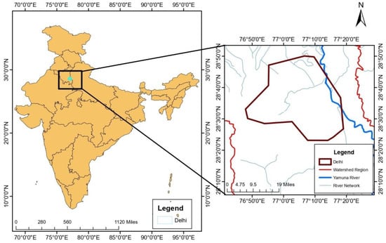
Figure 1.
Shows the study area map.
2.2. Data Collection
Data collection for the study region in Delhi for rainfall forecasting entails obtaining daily rainfall data from 1980 to 2021. These data are obtained from India’s Water Resources Information System (WRIS), a comprehensive database operated by the Ministry of Jal Shakti, Government of India. WRIS delivers an extensive amount of hydrological and meteorological information, including historical rainfall observations, which is critical for doing time series analysis for rainfall forecasting. WRIS daily rainfall data spanning four decades, from 1980 to 2021, were collected. A large time series is essential for capturing seasonal patterns, identifying trends, and understanding the historical behavior of rainfall in the studied region [63].
2.3. Data Preprocessing
To uphold the rigor of the analysis, the dataset was meticulously preprocessed. Initially, a comprehensive data cleansing step is performed to detect potential anomalies and inconsistencies. It is critical to highlight that while detecting outliers and missing values, none are removed, ensuring the dataset’s integrity remains intact. Data validation is carried out using statistical tools to ensure the dataset’s fidelity. Feature engineering plays a pivotal role in preprocessing. Leveraging the date variable to extract temporal features is essential for revealing patterns in rainfall predictions. Specifically, lag features were created that represent previous rainfall records, indicating the significance of historical data on subsequent forecasts. For this study, data from the preceding week are utilized to establish these lag features.
2.4. Creating Lagged Features
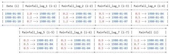
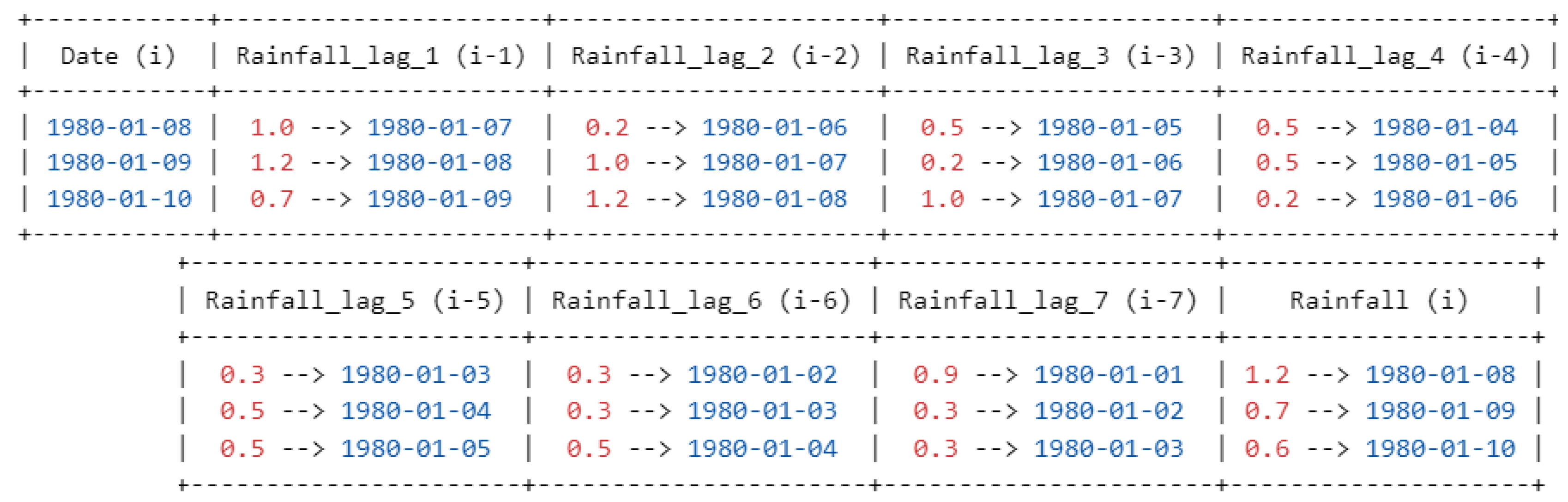
Time series forecasting leverages historical data to predict future events. One of the essential tools in this domain is the use of “lagged features”. By definition, a lagged feature at a specific time point encapsulates the data value from a previous period. This encapsulation enables predictive models to look back in time and use that historical context to make accurate forward projections. Consider a practical example: to forecast the rainfall for tomorrow, data from today would be termed “lag-1”, meaning it’s one day prior to the prediction point. Similarly, two days back, it is termed “lag-2”, three days back is “lag-3”, and so on, up to “lag-7” for a week ago.
This strategy is not arbitrary; it is deeply grounded in the inherent temporal structure of these data. Such lagged features act as historical markers, and by incorporating them, models become more attuned to the rhythms, patterns, and nuances of past data. This history-oriented approach prepares the model to anticipate and capture potential future patterns or trends. In the present research study, two distinct models were developed based on these lagged features, which differ in their time scale and input features. The details of these models are presented in Table 1, i.e., Model-1 for the daily dataset and Model-2 for the weekly data set [64].

Table 1.
Shows the model formulation of the current study.
Where “” is the date (for the daily model) or week (for the weekly model) for which the rainfall is predicted. The terms , , , etc., are the rainfall data from one, two, three, etc., days (for the daily model) or weeks (for the weekly model) before the prediction date or week. is the output or the predicted rainfall value for a date “” (for the daily model) or week “” (for the weekly model).
For Model-1, the focus is on leveraging daily lagged features. In this setup, each day is represented by the symbol “”. The model uses rainfall data from the previous seven days ( to) as input features. For instance, to predict the rainfall for a particular day, “,” the model would consider the rainfall data from the immediate previous day (), two days ago (), and so on until a week ago (). This allows the model to capture short-term fluctuations and patterns in the rainfall data.For example, for daily data formulation is shown in Scheme 1:
Scheme 1.
Shows the daily model formulation.
While Model-1 is designed around daily observations, Model-2 operates on a weekly scale. Despite using the same “” notation, in this context, each “” represents an aggregated or average value for a week. To predict the rainfall for the week “,” the model might use aggregated or average rainfall data from the previous seven weeks, i.e., (, , …,). This longer window allows the model to discern broader trends in the data, as weekly aggregates tend to be less noisy and more stable than daily figures.
The foundation of robust time series analysis is deeply rooted in the meticulous preparation and structuring of these data. Recognizing the intrinsic characteristic of time series data, which encapsulates a sequence of data points measured at successive points in time, to employ a time series split to partition the dataset, ensuring its integrity by maintaining its inherent chronological order. This is paramount in preserving the temporal relationships embedded within these data. In the present study, the earliest 70% of observations are used for the training set to develop the predictive models. Following these training data, the subsequent 15% are used as the validation set, essential for refining the models and ensuring the models do not overfit. The remaining 15%, which comprise the most recent observations, are designated as the test set and play a crucial role in assessing the real-world performance of the models in forecasting future rainfall patterns [64].
However, for models to provide accurate and dependable predictions, raw data, particularly from disparate sources, must be standardized. Raw datasets, with their intrinsic differences in scale, units, and magnitude, might introduce bias inadvertently. To address this issue, the current study implemented a comprehensive pipeline that smoothly incorporates a StandardScaler. This method standardizes the dataset by removing the mean and scaling characteristics to unit variance, resulting in a harmonized input in which all features comply with a common scale. This type of standardization not only improves computational speed but also assures that each feature contributes consistently to the predictive process. The preprocessing regimen, which includes strategic time series segmentation and feature standardization, is intended to increase the dependability and accuracy of forecasts.
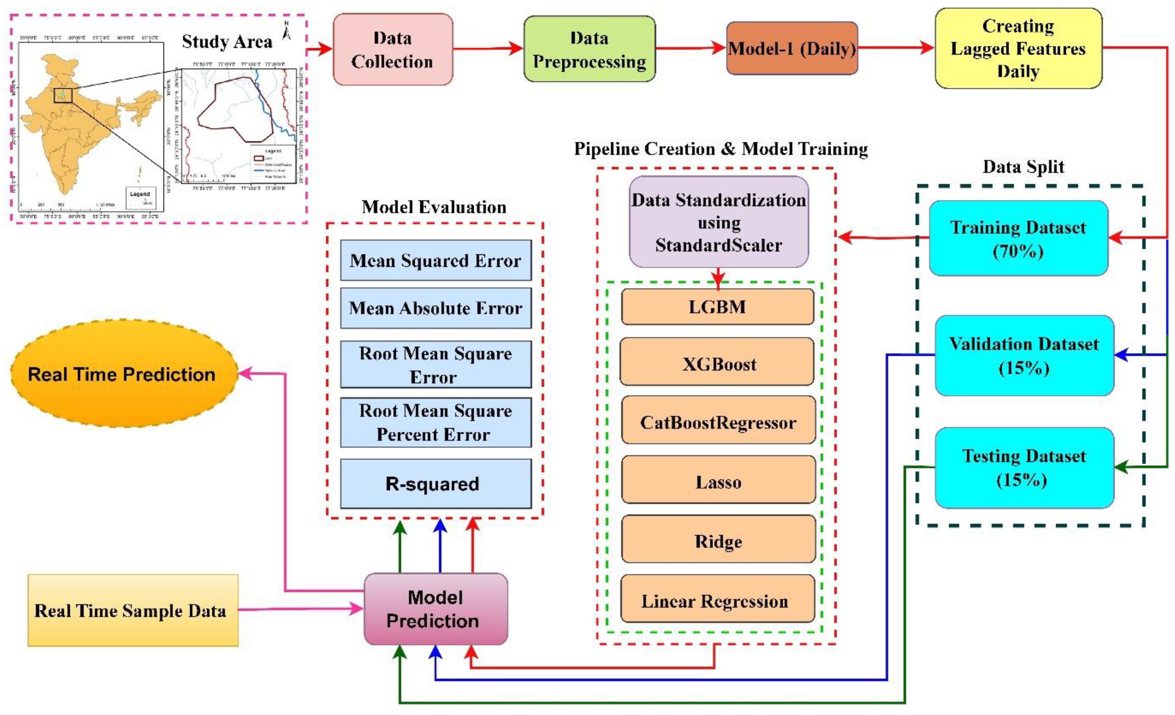
Figure 2 provides a flowchart illustrating the implementation of Model-1, which uses daily data. The subsequent steps detail the process:
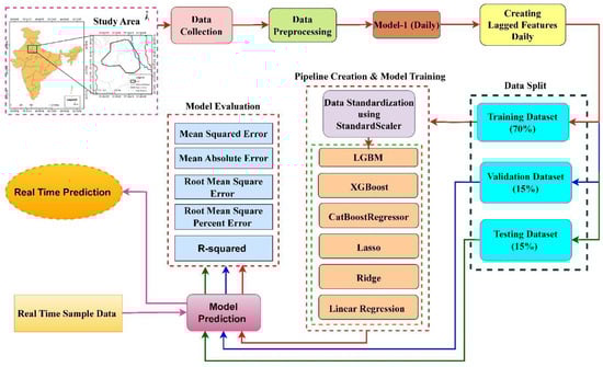
Figure 2.
This flowchart outlines each stage in the implementation of Model 1, which is based on daily data.
- Start:Label: “Begin Research (Study area)”
- Data Collection & Preprocessing:Label: “Data Collection & Preprocessing”Sub-points:
- Raw data acquisition
- Data cleaning
- Outlier handling
- Feature engineering (Creating lagged features)
- Data Splitting
- Pipeline Creation & Model Training:Label: “Establish Pipeline & Train Model”Sub-points:
- Data Standardization using StandardScaler
- Model Estimation (Training)
- Models used: CatBoost, Lasso, LGBM, Linear Regression, Ridge, and XGBoost
- Model Evaluation:Label: “Evaluation of Model Predictions”Sub-points:
- Evaluation Metrics
- Visualization: Error plots, Prediction plots
- Conclusion:Label: “Draw Conclusions & Derive Insights”
- End:Similar steps are followed for model 2 (weekly data).
3. Methodology and Methods
Machine learning rainfall forecasting entails a systematic process for using past weather data and important meteorological factors to make reliable forecasts. The first phase is data collection, which involves gathering historical meteorological data, such as daily or hourly rainfall observations. The dataset is preprocessed after data collection to ensure data quality and uniformity. Data preparation deals with missing values, eliminating outliers, and normalizing data so that they may be analyzed and modeled. Following the data cleaning, the next phase is feature selection and engineering. This stage entails finding the most important climatic factors that influence rainfall patterns. Creating new features or altering old ones to capture intricate interactions between variables and rainfall is another aspect of feature engineering. The right machine learning model must be chosen based on the unique rainfall forecasting problem. The testing dataset is used for model evaluation to examine the model’s accuracy and predictive capabilities. Once the model has been tested and reviewed, it is ready to estimate rainfall for future time periods. Depending on the application, these forecasts can be used for short-term (e.g., daily), medium-term (e.g., weekly), or long-term (e.g., seasonal) predictions. The trained and approved machine learning model is subsequently implemented in real-world applications for operational usage. As weather patterns and data distributions vary over time, continuous monitoring of the model’s performance is required to guarantee that it stays accurate and up to date.
3.1. Light Gradient-Boosting Machine Regressor (LGBM)
The LGBM gradient-boosting approach is widely known for its efficacy and versatility. It includes a variety of improvements and upgrades to improve gradient-boosting performance on large datasets [65]. During the data preparation phase, training data are partitioned into input features and target values, particularly intended for regression analysis. It is recommended to utilize target values alongside metric attributes. Following that, all parameters—including learning rate, tree count, maximum depth, and feature percentage—are set. These parameters, which may be changed to enhance performance, affect how the LGBM model behaves. The process of building and training a model involves the creation of a series of decision trees. A gradient-driven optimization method is employed to minimize the loss function while constructing each tree. The model’s predictions undergo updates based on the gradients derived from the loss function, and the collection of trees is iteratively expanded. The model may be used to predict fresh data points after training. The LGBM technique employs a weighted summation to amalgamate predictions from individual trees within the ensemble. During the training iteration, these weights are established through evaluations of the loss function’s gradients. The subsequent equation can be employed to predict the target variable using LGBM:
where, forecasts the goal value, the weight assigned to the th tree is denoted by , and the forecast made by the th tree for the input attributes is represented by . Massive datasets can be handled by the LGBM, and it excels at capturing intricate non-linear connections between features and the target variable. Through gradient-based optimization, it constructs a set of trees that collectively yield accurate predictions, thus enhancing the performance of the loss function.
3.2. Extreme Gradient-Boosting Regression Model (XGBoost)
XGBoost stands as a potent ensemble learning technique primarily utilized for regression modeling. It predicts using gradient boosting and decision trees. The XGBoost technique improves performance in several ways while sharing a similar structure with other gradient-boosting regressors [66]. The following sections discuss the XGBoost algorithm:
- The initial stage involves choosing parameters for the XGBoost model, which encompasses elements such as learning rate, tree count, maximum depth, and feature fraction. Modifying these parameters can enhance performance and exert control over the model’s behavior.
- Train the model: The XGBoost model is formed by assembling numerous decision trees. Every tree is meticulously constructed using a gradient-guided optimization method that seeks to minimize the loss function. As the training progresses, the collection of trees is consistently expanded, and predictions are adjusted based on gradients within the loss function.
- Following model training, the model may be utilized to forecast new data points. To produce the final regression prediction, the XGBoost approach includes the predictions from each tree in the ensemble. The loss function employed determines the specific approach for merging the predictions.
- The formula for making predictions using an XGBoost regression model can be summarized as follows: Given an XGBoost regression model with trees: Each tree is denoted as. represents the input features. The predicted output from the XGBoost model is obtained by aggregating the predictions from all individual trees:where: represents the prediction of the th tree on input .
3.3. CatBoostRegressor Algorithm
CatBoostRegressor is a machine-learning method that uses gradient-boosted decision trees to forecast continuous variables. The CatBoostRegressor is renowned for its effectiveness, accuracy, and ability to handle categorical variables [67]. A collection of weak decision trees must first be constructed for the CatBoostRegressor method to work. After that, these trees are combined to create a strong model. The technique used to connect the trees is gradient boosting. Gradient boosting corrects the errors made by the prior trees by adding new trees to the model. Equation (3) displays the formula that CatBoostRegressor uses to forecast continuous values:
Here, represents the predicted value while denotes the input features. The resultant function is a linear amalgamation of fundamental functions, . The coefficients ascertain the significance of individual base functions within this linear amalgamation.
The model coefficients are computed using the gradient descent technique. In the CatBoost, the loss function needs to be reduced. The loss function calculates the discrepancy between the expected values and the actual values. The powerful ML technique CatBoost may be used to handle a variety of regression issues. It works particularly well for problems involving categorical properties.
3.4. Lasso
Lasso, frequently referred to as L1 regularization, represents a type of linear regression model that incorporates a penalty element based on the L1 norm of coefficients. This can drive specific coefficients to become precisely zero; feature selection is accomplished by encouraging sparsity in the coefficient values [68]. The following may be used to depict the Lasso regression formula using Equation (4):
A regularization term is included in the objective function of Lasso regression together with the mean squared error (MSE) factor:
where y is the dependent variable and , , …, and are the independent variables (input characteristics). The coefficients (parameters) of the independent variables are , , …, . The regularization parameter, which is, determines the intensity of the regularization. The right balance between penalizing the coefficient size ( norm) and fitting these training data (MSE term) is selected.
The L1 norm term for the objective function is created by summing the absolute values of the coefficients.
Lasso regression endeavors to discover ideal coefficient values that decrease the Mean Squared Error (MSE) term while simultaneously minimizing the L1 norm term within the scope of the overall objective function minimization. Consequently, specific coefficients could potentially be driven to zero, leading to the removal of corresponding features from the model. This unique characteristic empowers Lasso regression to efficiently handle datasets with high dimensionality and assist in feature selection.
3.5. Ridge
Ridge regression is a prevalent machine learning technique frequently applied within the realm of supervised learning for tasks involving regression analysis. To deal with the multicollinearity and overfitting concerns, regression analysis usually utilizes Ridge regression, also known as Tikhonov regularization. It represents an advancement over ordinary least squares (OLS) regression, modifying the loss function through the introduction of a regularization term [69]. The equation for Ridge regression is stated as follows:
In this equation, the Euclidean norm is represented as , the target variable is denoted as , the predictor variables as , the coefficients as and the regularization parameter as . Ridge regression penalizes the magnitudes of the coefficients (), simultaneously working to minimize the sum of squared differences between predicted and actual values .
3.6. Linear Regression (LR)
LR technique that handles a collection of records with and values. The goal of regression is to determine the value of provided that is continuous. Regression may be performed using a variety of functions or models, but the most common is the linear function [70].
where stands for intercept, for coefficient, and stands for the input training data. stands for the projected value of given . The best-fit line may be found once the ideal values of and have been established.
4. Model Evaluation
Evaluate the performance of the trained model using the validation dataset. Predictions are generated using these validation data and subsequently compared with the actual observations. Several evaluation metrics, including Mean Squared Error (MSE), Mean Absolute Error (MAE), Root Mean Square Error (RMSE), Root Mean Square Percent Error (RMSPE), and R-squared (), are employed for assessment.
Here, signifies the overall count of data points. The actual (observed) value of the dependent variable for the th data point is denoted as . On the other hand, represents the anticipated value of the dependent variable for the th data point. Σ symbolizes the summation of squared deviations for each data point. The symbol signifies the mean of the dependent variable.
5. Results and Discussion
5.1. Results and Discussion of Model-1
Model-1 depicts the daily data time series rainfall forecast. CatBoost, Lasso, LGBM, Linear Regression, Ridge, and XGBoost are among the models tested in this study. MAE, MSE, RMSE, RMSPE, and R2 are the assessment metrics used to analyze these models’ performances.
5.1.1. Performance Metrics of Training Data for Model-1
Table 2 displays the performance characteristics of various machine learning models for rainfall predictions using training data. CatBoost outperforms the other models on training data with extremely low MAE, MSE, and RMSE values. It produces a nearly flawless R2 value near one, suggesting a great fit to these training data. A RMSPE score of roughly 0.49 implies that the forecasts have a low percentage of errors. While Lasso performs reasonably well, it has greater MAE, MSE, and RMSE values than CatBoost. The R2 value of about 0.71 indicates that the model accounts for approximately 71% of the variation in these training data. However, the rather high RMSPE value of about 383 implies that the forecasts contain errors. LGBM performs well as well, with low MAE, MSE, and RMSE values. An R2 value of roughly 0.99 indicates a good fit for these training data. The RMSPE score of roughly 26 suggests that the prediction percentage errors are reasonably modest. Linear Regression and Ridge models perform similarly on training data, with relatively low MAE, MSE, and RMSE values. values of around 0.83 show that these models explain around 83% of the variation in these training data. The RMSPE values of around 179 are greater compared with prior models, indicating some percentage error in the forecasts. XGBoost performs admirably as well, with low MAE, MSE, and RMSE values. The value of around 0.99 suggests a good fit to these training data. However, the slightly higher RMSPE value of around 0.94 than Catboost shows that there are some percentage errors in the forecasts.
Table 2.
Model-1 training dataset results.
5.1.2. Performance Metrics of Validation Data for Model-1
Table 3 shows the machine learning models’ performance metrics on the validation dataset for rainfall forecasting for Model-1. CatBoost continues to outperform on the validation dataset, with very low MAE, MSE, and RMSE values, as on these training data. It produces a nearly flawless R2 value around one, suggesting a great fit to these validation data. The RMSPE value of roughly 0.48 suggests that the percentage errors in the predictions on the validation dataset are reasonably low. Lasso, on the other hand, performs poorly on the validation dataset with higher MAE, MSE, and RMSE values than CatBoost. The score of about 0.71 indicates that the model accounts for approximately 71% of the variation in these validation data. The RMSPE score of about 372 suggests some percentage errors in the validation dataset predictions. LGBM performs well on the validation dataset as well, with low MAE, MSE, and RMSE values. An R2 score of 0.99 shows a good fit for these validation data. The RMSPE score of about 25 indicates that the percentage errors in the predictions on the validation dataset are quite low. On the validation dataset, the Linear Regression and Ridge models perform similarly, with low MAE, MSE, and RMSE values. R2 values of around 0.83 show that these models explain around 83% of the variation in these validation data. The RMSPE values of around 173 are higher than in other models, indicating more percentage errors in the validation dataset predictions. On the validation dataset, XGBoost likewise performs well, with low MAE, MSE, and RMSE values. The R2 value of around 0.99 shows a good match to these validation data. The RMSPE score of roughly 0.92 indicates that the percentage errors in the predictions on the validation dataset are quite low.
Table 3.
Model-1 validation dataset results.
5.1.3. Performance Metrics of Testing Data for Model-1
Table 4 displays the performance metrics for the machine learning models for rainfall forecasting on the testing dataset of Model-1. CatBoost continues to outperform on the testing dataset, as demonstrated in earlier assessments on the training and validation datasets, with very low MAE, MSE, and RMSE values. It produces a nearly flawless R2 score of around 1, suggesting an outstanding match to these testing data. The RMSPE score of roughly 0.49 indicates that the percentage errors in the predictions on the testing dataset are quite low. Lasso, on the other hand, performs poorly as compared with CatBoost on the testing dataset, with higher MAE, MSE, and RMSE value errors. The R2 score of around 0.71 indicates that the model accounts for approximately 71% of the variation in the tests. The RMSPE score of about 387 suggests that the predictions on the testing dataset have some percentage errors. LGBM also performs well on the testing dataset, with low MAE, MSE, and RMSE values. An R2 score of 0.99 shows a good match to these testing data. The RMSPE score of around 25 indicates that the percentage errors in the predictions on the testing dataset are reasonably low. Linear Regression and Ridge models continue to perform similarly on the testing dataset with poor results as compared with other methods. R2 values of around 0.83 imply that these models explain around 83% of the variation in these testing data. When compared with other models, the RMSPE values of about 177 are higher, indicating percentage errors in the predictions on the testing dataset. On the testing dataset, XGBoost maintains its high performance with low MAE, MSE, and RMSE values. The R2 score of around 0.99 shows a good match to the testing data. The RMSPE score of roughly 0.95 indicates that the percentage errors in the predictions on the testing dataset are reasonably low.
Table 4.
Model-1 testing dataset results.
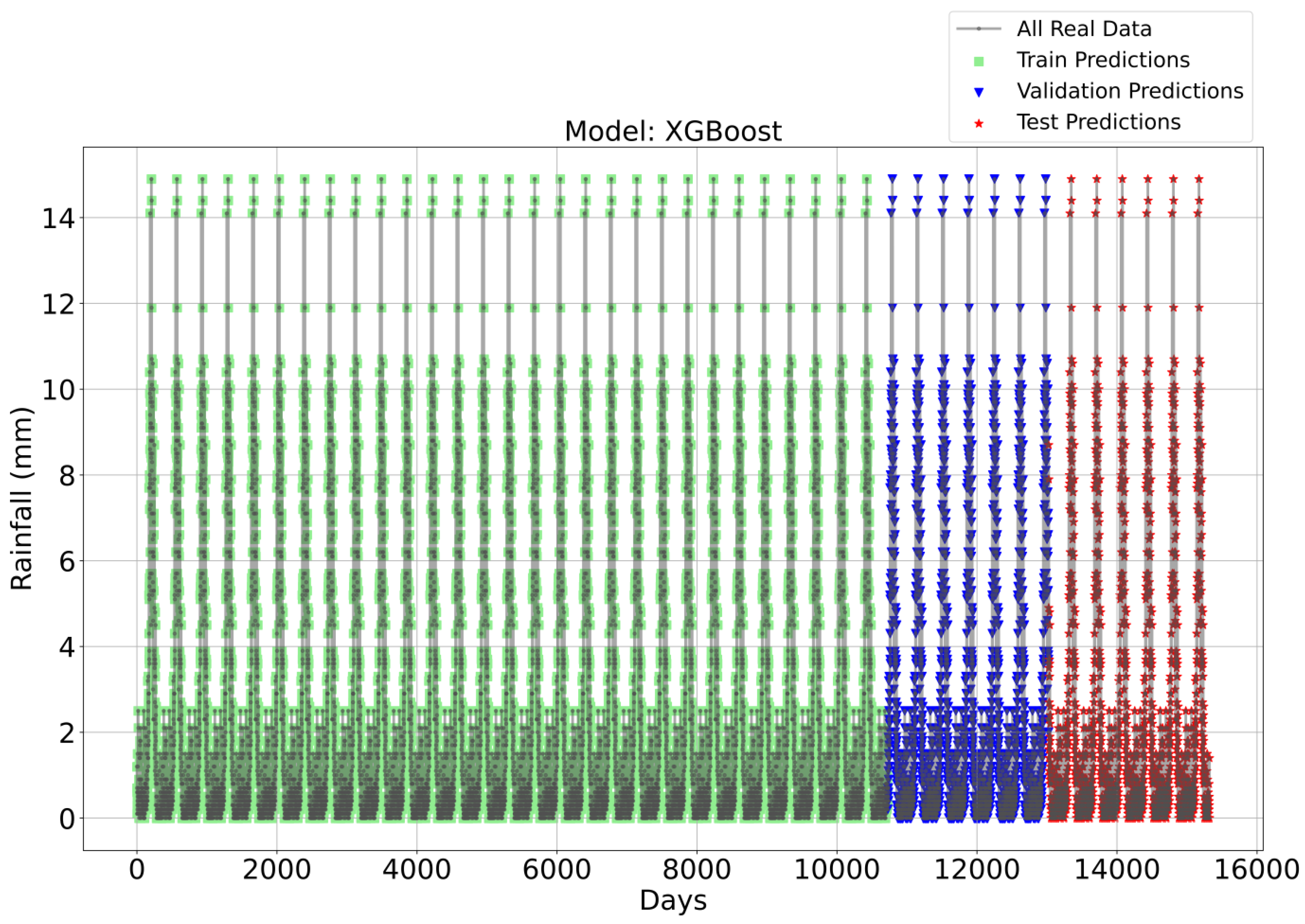
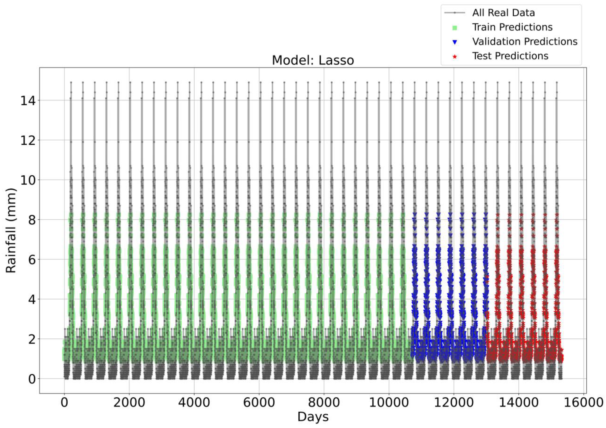
5.1.4. Comparison of the algorithms in Model-1
Figure 3, Figure 4, Figure 5 and Figure 6 illustrate the time series prediction for (CatBoost, LGBM, XGBoost, and Lasso) for Model-1, with predicted rainfalls presented alongside actual data. CatBoost consistently outperforms all other models in all three datasets: training, validation, and testing for Model-1. It produces accurate and dependable rainfall forecasts, making it the best model for rainfall forecasting in the study region for daily data. The ensemble-based models (LGBM and XGBoost) also perform well, but CatBoost outperforms them. Linear Regression, Lasso, and Ridge models perform poorly and lack the precision and consistency of ensemble-based models such as CatBoost. Figure 6 depicts the Lasso time series forecast; it can be observed that the maximum peaks are not achieved using this method. These findings show the importance of ensemble techniques in enhancing rainfall forecasting accuracy and highlight the potential of CatBoost and XGBoost as beneficial tools for meteorologists and policymakers.
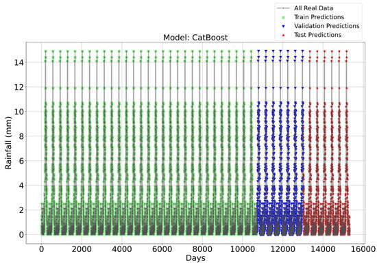
Figure 3.
Time Series forecasting for the CatBoost Model-1.

Figure 4.
Time Series forecasting for the LGBM Model-1.
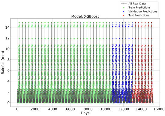
Figure 5.
Time Series forecasting for the XGBoost Model-1.

Figure 6.
Time Series forecasting for the Lasso Model-1.
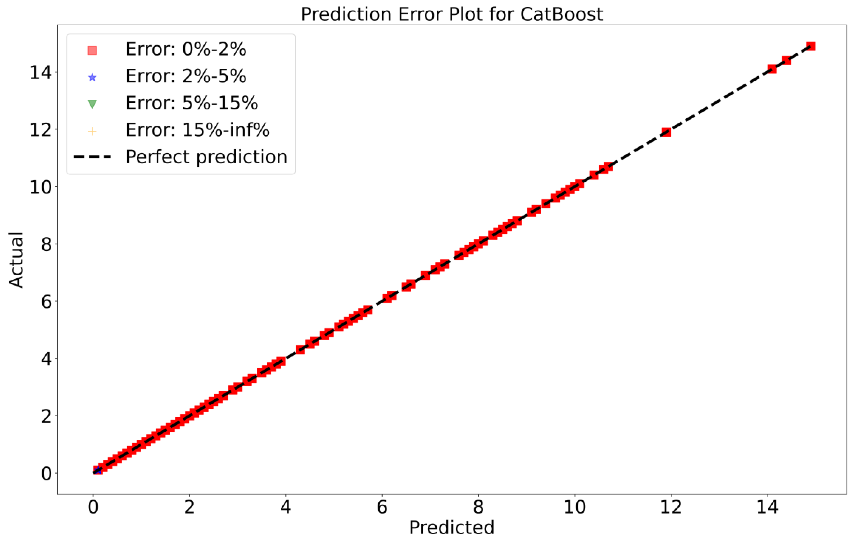
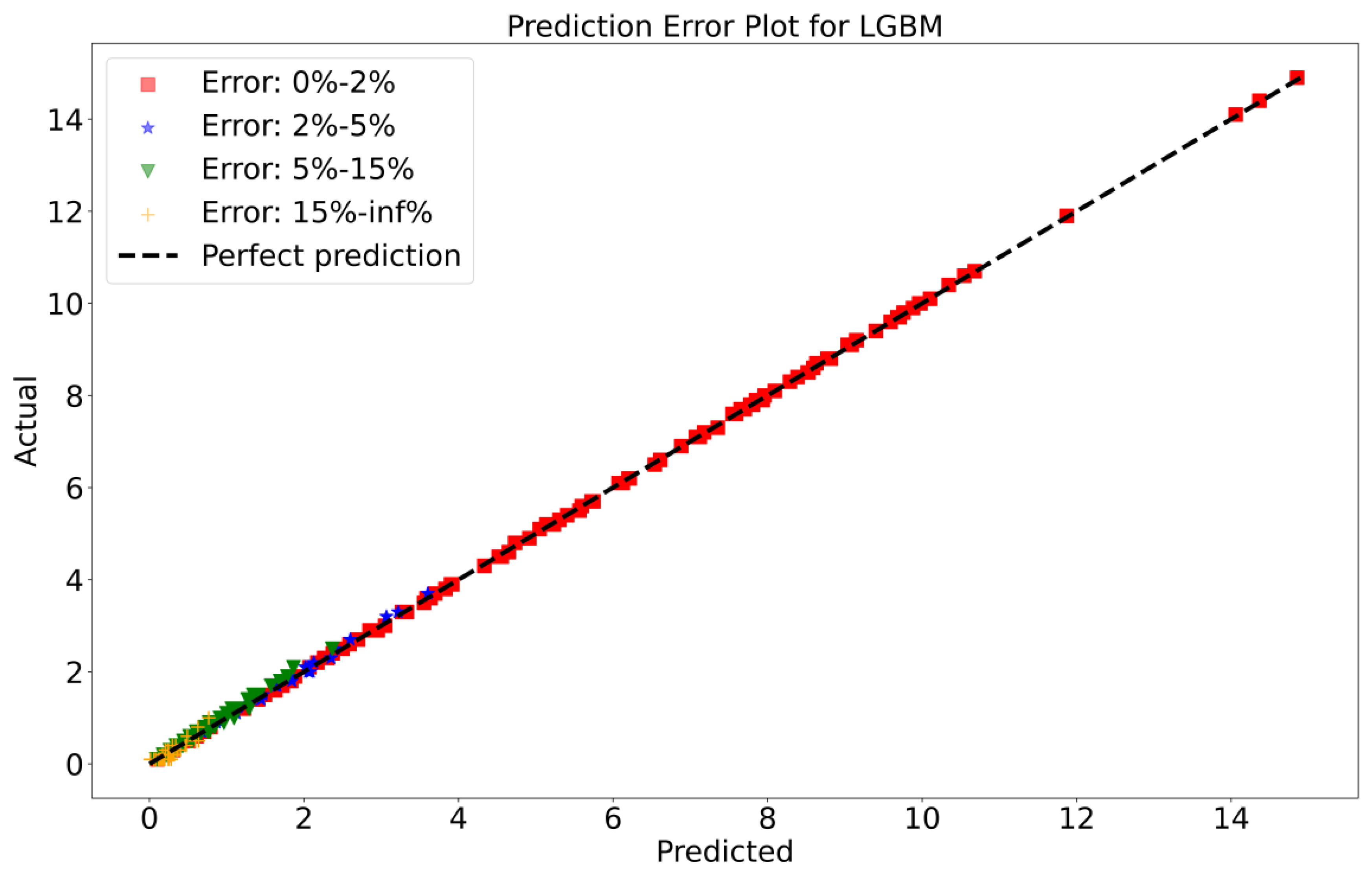
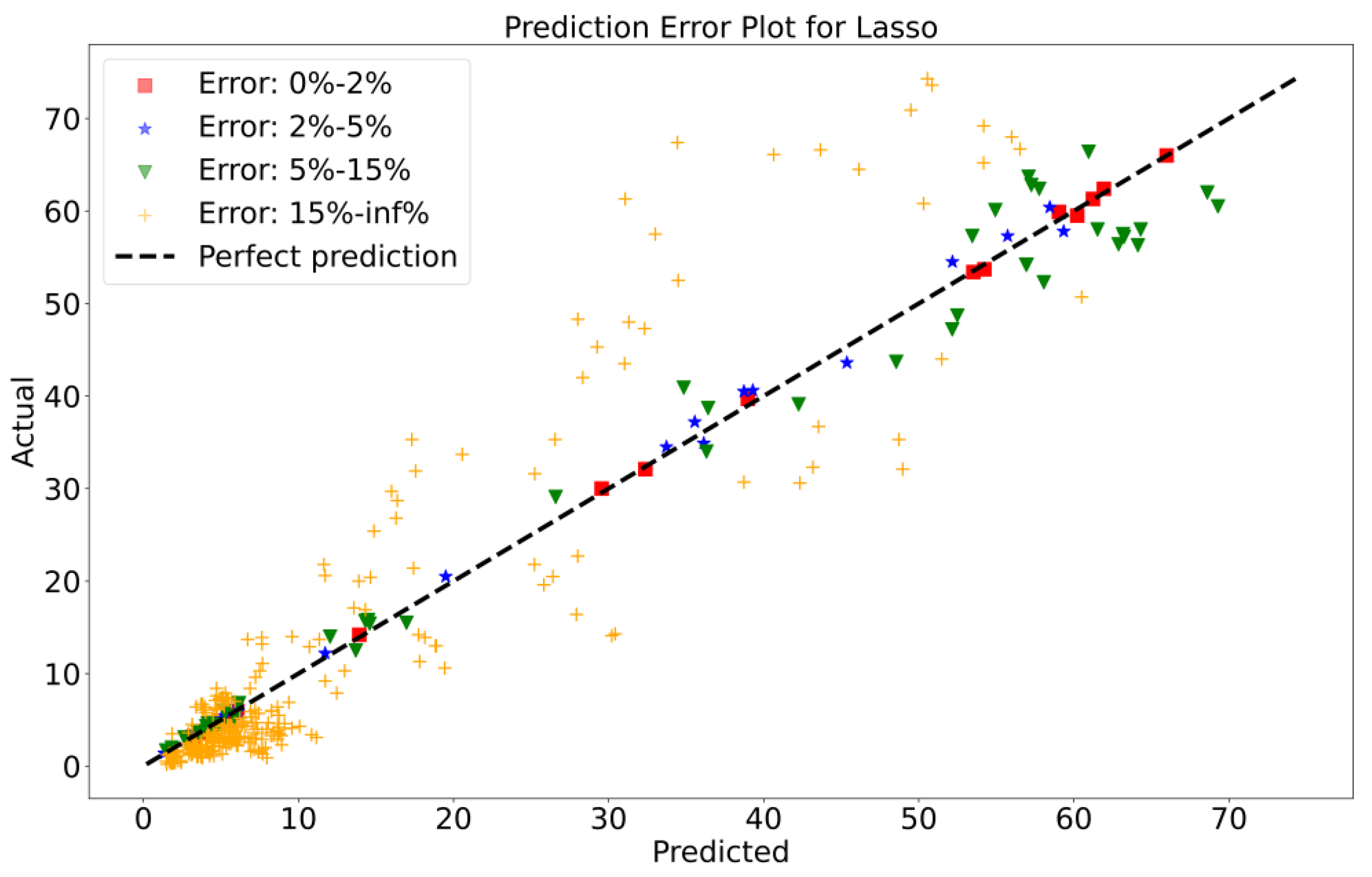
To attain a better understanding of CatBoost, LGBM, XGBoost, and Lasso, error scatter plots (shown in Figure 7, Figure 8, Figure 9 and Figure 10) have been developed to highlight the association between predicted and actual rainfall for CatBoost, LGBM, XGBoost, and Lasso. An investigation of these figures suggests that a data point error of less than 0 to 2% has been recorded. LGBM shows a greater percentage of data point errors ranging from 2% to 15% for rainfall data. Similarly, with XGBoost, data point errors range from 2% to 5% for rainfall data; however, very little error was detected for CatBoost. Lasso shows the highest percentage of data point errors, with values greater than 15% for rainfall data. Taking all these aspects into account, it is fair to say that the CatBoost model outperformed both XGBoost and LGBM in terms of robustness and dependability for daily rainfall predictions.

Figure 7.
Scatter plots of rainfall forecasting for the CatBoost Model-1.

Figure 8.
Scatter plots of rainfall forecasting for the LGBM Model-1.

Figure 9.
Scatter plots of rainfall forecasting for the XGBoost Model-1.
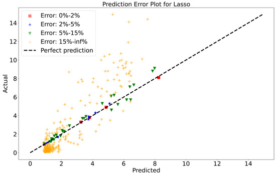
Figure 10.
Scatter plots of rainfall forecasting for the Lasso Model-1.
5.2. Results and Discussion of Model-2
Model-2 shows the rainfall forecast of the weekly data time series. The models evaluated include CatBoost, Lasso, LGBM, Linear Regression, Ridge, and XGBoost. The evaluation metrics used to assess the models’ performance are MAE, MSE, RMSE, RMSPE, and R2.
5.2.1. Performance Metrics of Training Data for Model-2
Table 5 displays the performance characteristics of multiple machine learning models for the “Model-2” training dataset for rainfall forecasting. XGBoost and CatBoost outperform the other models in the training dataset across various assessment measures. These two models consistently outperform others in terms of MAE, MSE, RMSE, RMSPE, and R2. CatBoost obtains an exceptionally low MAE of 0.049 and an equally amazing RMSE of 0.083, confirming its prediction accuracy. XGBoost outperformed CatBoost with an even lower MAE of 0.014 and an RMSE of 0.055. These numbers indicate XGBoost’s capacity to decrease prediction errors and give a strong fit to these training data. Furthermore, both models had R-squared values of 0.99, indicating their ability to explain the variation in these training data. This means they capture a significant amount of the underlying patterns in the dataset, resulting in good prediction performance. LGBM also performs well on the training dataset, with low MAE, MSE, and RMSE values. An R2 score of 0.99 shows a good match to these training data. In comparison, while Lasso, LR, and Ridge produce acceptable results, they fall short of CatBoost, XGBoost, and LGBM. These models have greater MAE, RMSE, and RMSPE values, indicating a less-than-optimal fit to these training data. Based on a thorough examination of the assessment criteria in Table 5, XGBoost emerged as the best model for the training dataset. Continually decreased errors and higher R-squared values demonstrate their stability and accuracy in capturing the underlying connections among these data.
Table 5.
Model-2 training dataset results.
5.2.2. Performance Metrics of Validation Data for Model-2
Table 6 shows that CatBoost and XGBoost remain the most proficient models among the tested alternatives for the validation dataset. These two models outperform across different assessment measures. CatBoost has a surprisingly low MAE of 0.050 and an even lower RMSE of 0.081936. XGBoost outperformed CatBoost with an even lower MAE of 0.014 and an RMSE of 0.049. These numbers highlight the excellent predictive capabilities of CatBoost and XGBoost, significantly decreasing prediction errors and delivering a solid match to these validation data. Furthermore, both models have an R2 value of 0.99, confirming their ability to explain a large percentage of the variation in the validation dataset. This high R2 result suggests that these models can capture the underlying patterns and connections in these data. LGBM also performs well on the validation dataset, with low MAE, MSE, and RMSE values. An R2 score of 0.99 shows a good match to the validation dataset. In comparison, while Lasso, LR, and Ridge provide adequate performance, they fall short of CatBoost, XGBoost, and LGBM in terms of accuracy. These models have greater MAE, RMSE, and RMSPE values, indicating a worse fit to these validation data. Table 6 shows an extensive examination of the assessment metrics that confirms XGBoost as the best option among the models selected for the validation dataset. Its persistent capacity to obtain decreased errors, along with a very high R-squared value, demonstrates its dependability and precision in capturing the intricacies of these validation data.
Table 6.
Validation dataset results for Model-2.
5.2.3. Performance Metrics of Testing Data for Model-2
Table 7 shows that CatBoost and XGBoost consistently appear as the most resilient and accurate models among the alternative methods. These two models outperform in a variety of crucial assessment parameters. CatBoost’s predictive skill remains remarkable, with a very low MAE of 0.05 and a commendable RMSE of 0.12. Similarly, XGBoost outperformed CatBoost with an even lower MAE of 0.02 and an RMSE of 0.10. These results confirm XGBoost’s consistent ability to efficiently eliminate prediction errors and give a solid fit to these testing data. Furthermore, both models have an excellent R2 value of 0.99, demonstrating their ability to capture a significant percentage of the variation in the testing dataset. This strong R2 value demonstrates their ability to detect underlying patterns and correlations. LGBM also performs well on the validation dataset, with low MAE, MSE, and RMSE values. An R2 score of 0.99 shows a good match to the validation dataset. In comparison, while Lasso, LR, and Ridge provide adequate performance, they fall short of the accuracy displayed by CatBoost, XGBoost, and LGBM. These models have greater MAE, RMSE, and RMSPE values, implying a worse fit to these testing data. The full examination of the assessment measures in Table 7 confirms XGBoost as the best option among the models selected for the testing dataset. Their persistent capacity to obtain fewer errors, together with the extraordinarily high R2 value, reinforces their dependability and precision in capturing the complexities of the testing data.
Table 7.
Model-2 testing dataset results.
5.2.4. Comparison of the algorithms in Model-2
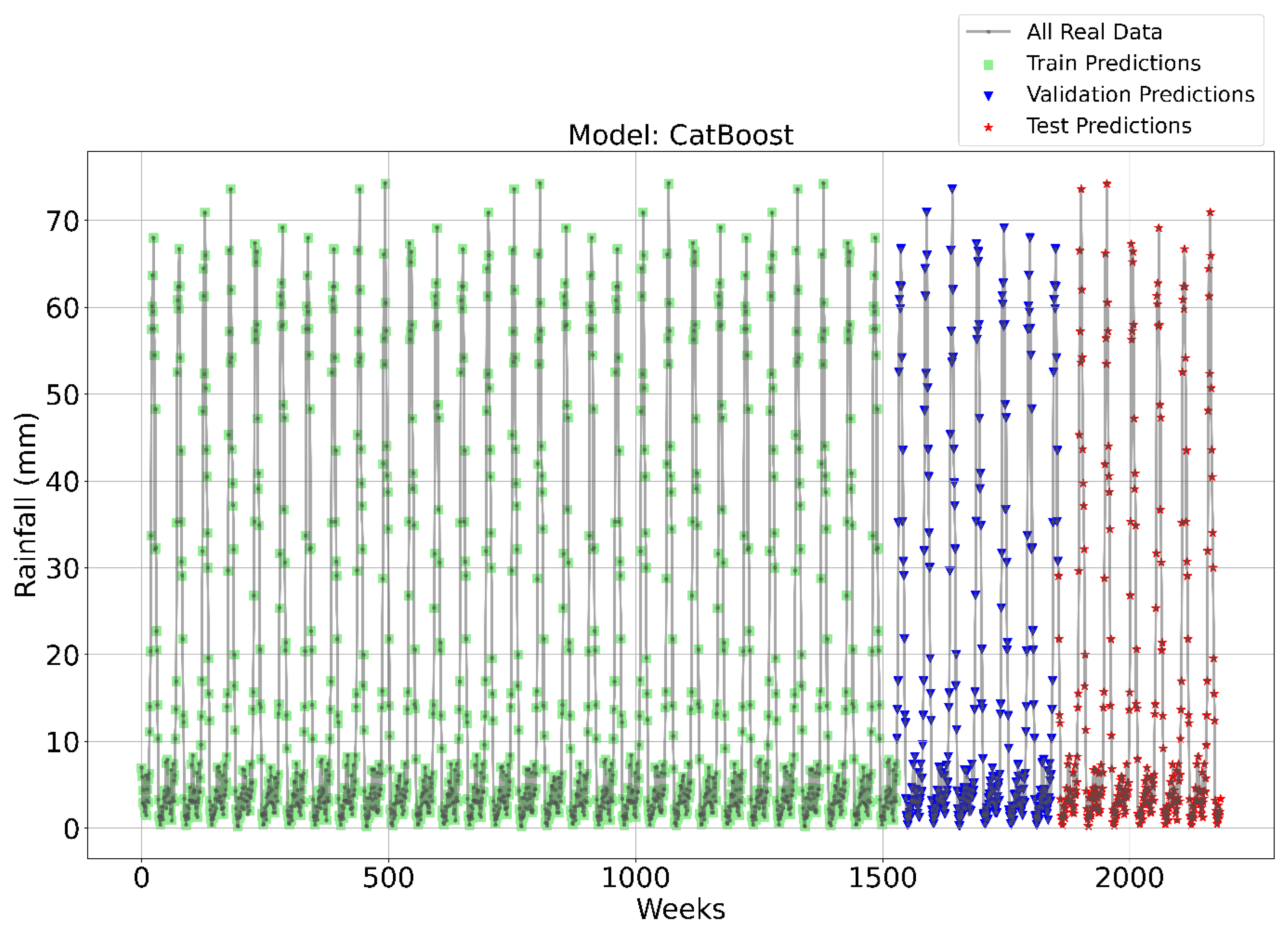
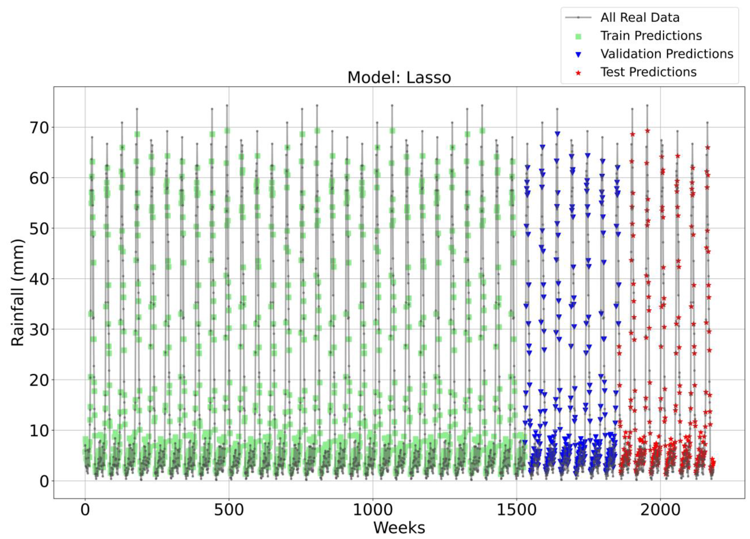
Figure 11, Figure 12, Figure 13 and Figure 14 illustrate the time series prediction for (CatBoost, LGBM, XGBoost, and Lasso) for Model-2, with predicted rainfalls presented alongside actual data. According to the comparisons, XGBoost consistently beat the other models on all three datasets (Training, Validation, and Testing). This model regularly shows reduced errors (MAE, RMSE) and higher R2 values, indicating improved prediction powers, resilience, and capacity to capture underlying data patterns. The CatBoost and LGBM also perform well, but XGBoost outperforms them. Although Lasso, LR, and Ridge perform poorly, they have greater errors and lower R2 values than CatBoost and XGBoost. Figure 14 depicts the Lasso time series forecast; it can be observed that the maximum peaks are not achieved by this method. This shows that CatBoost and XGBoost are the best choices for this task since they consistently perform the best overall across all three datasets.
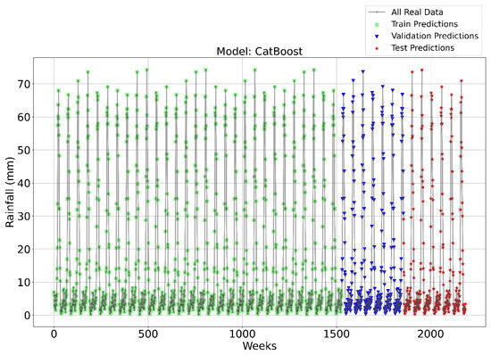
Figure 11.
Time Series forecasting for the CatBoost Model-2.
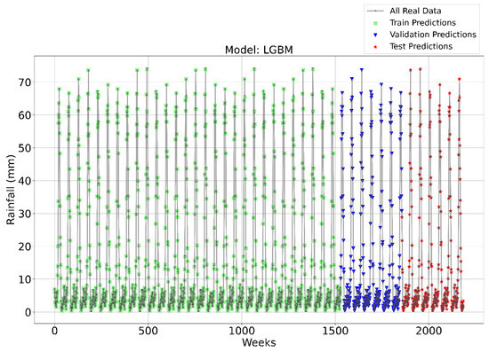
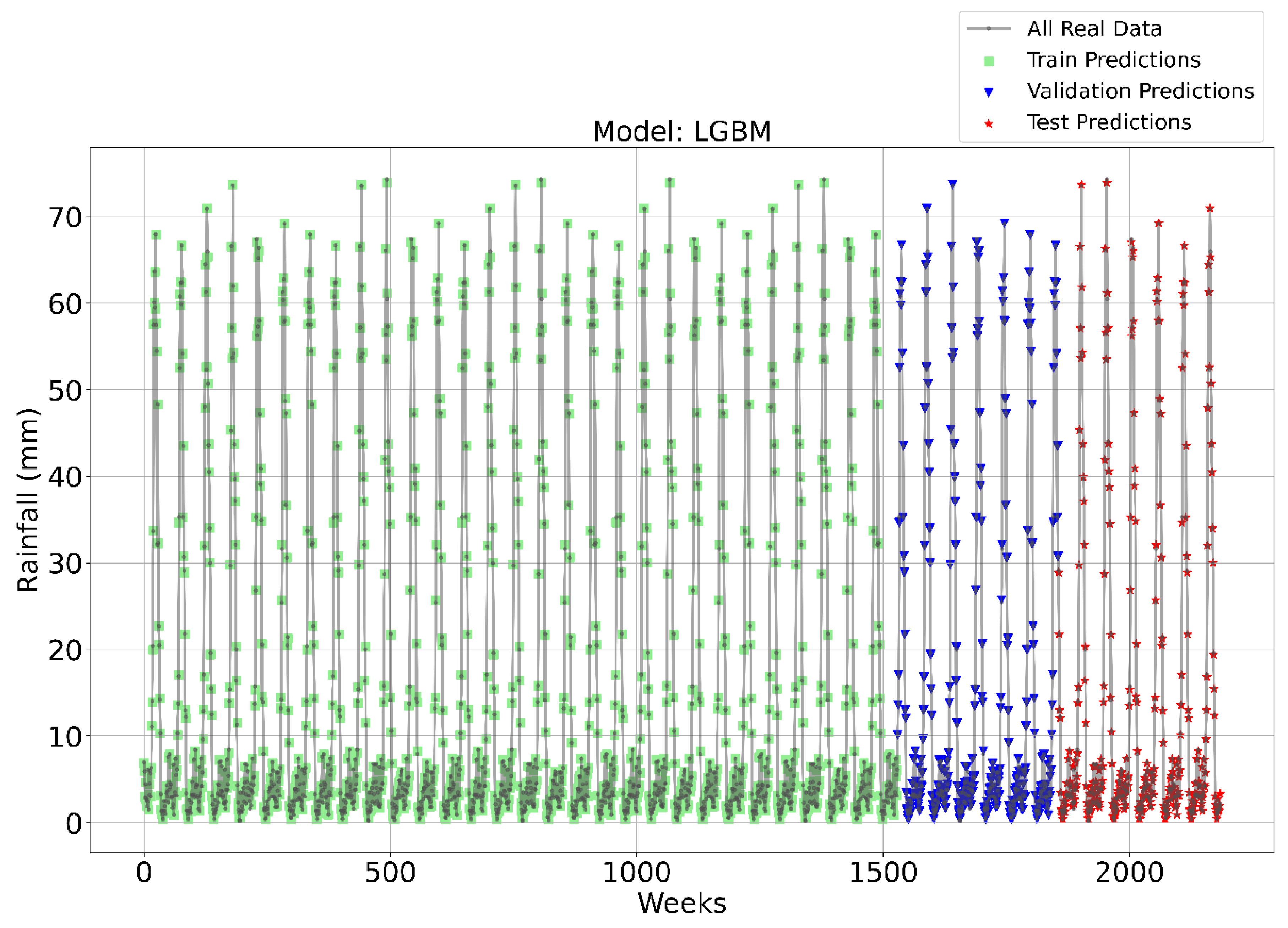
Figure 12.
Time Series forecasting for the LGBM Model-2.
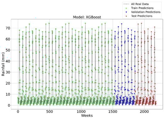
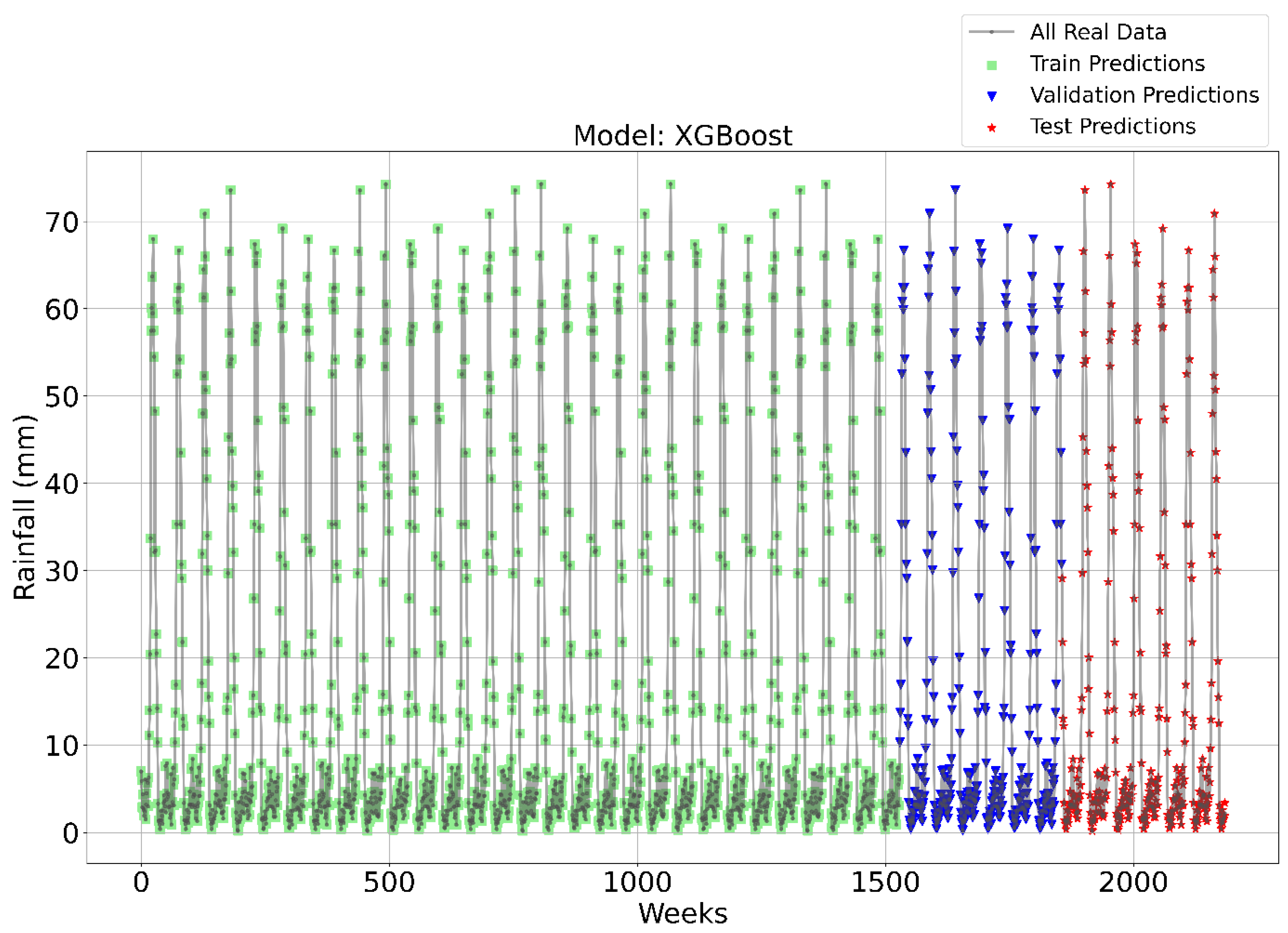
Figure 13.
Time Series forecasting for the XGBoost Model-2.
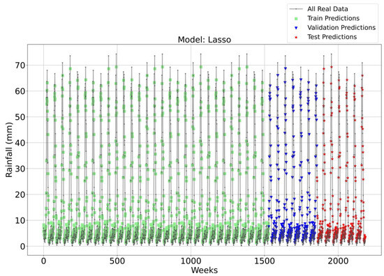
Figure 14.
Time Series forecasting for the Lasso Model-2.
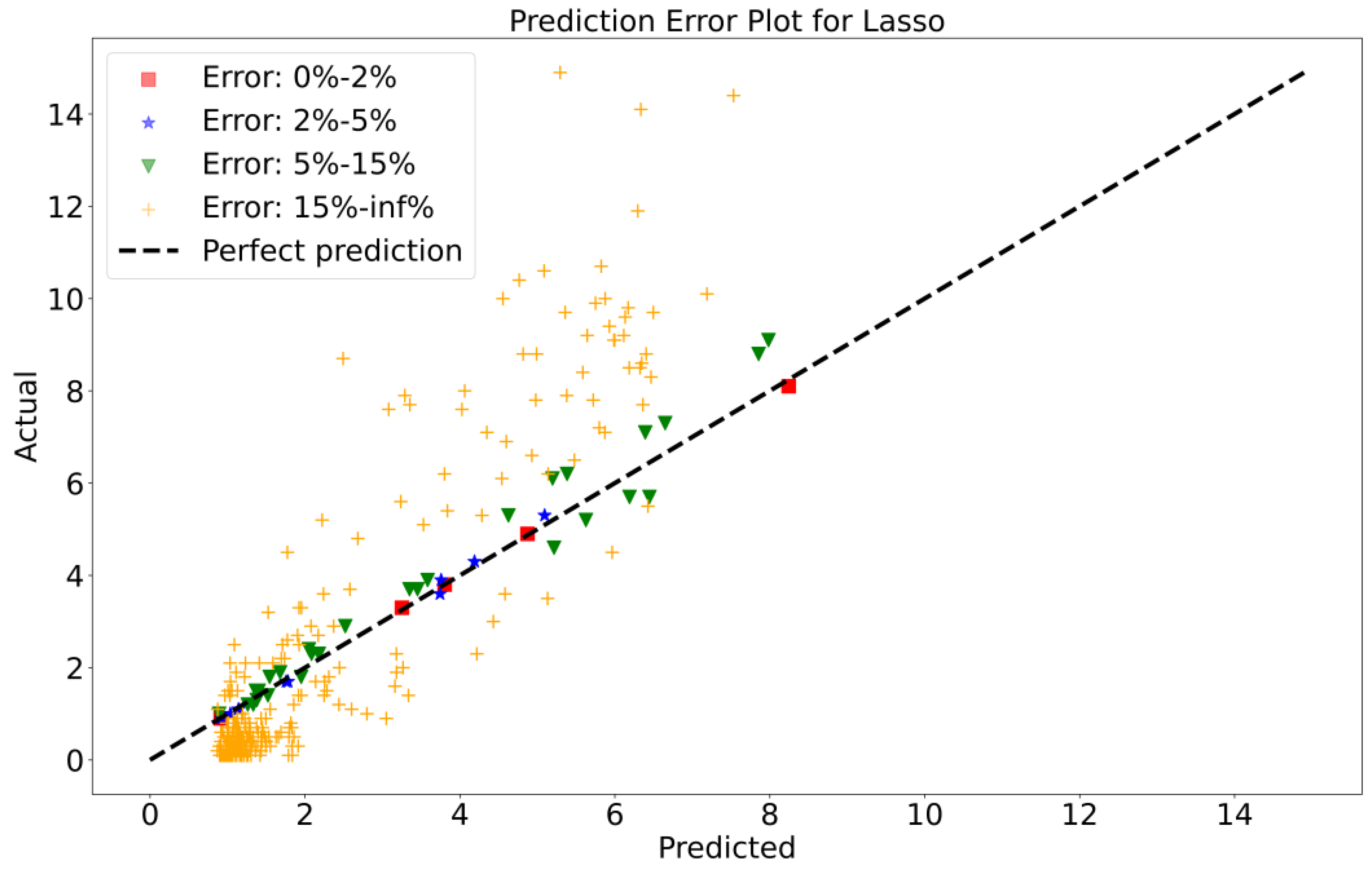
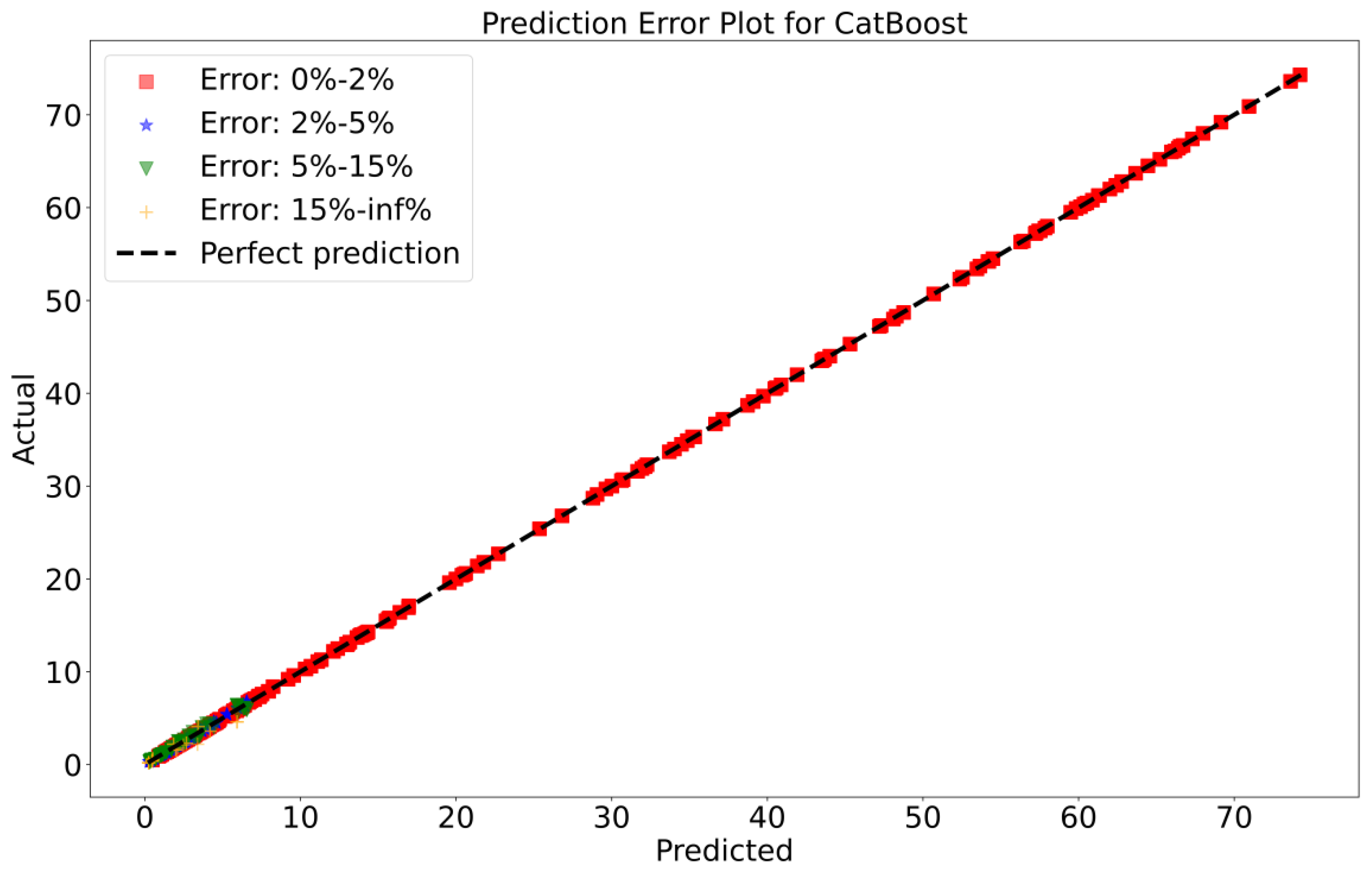
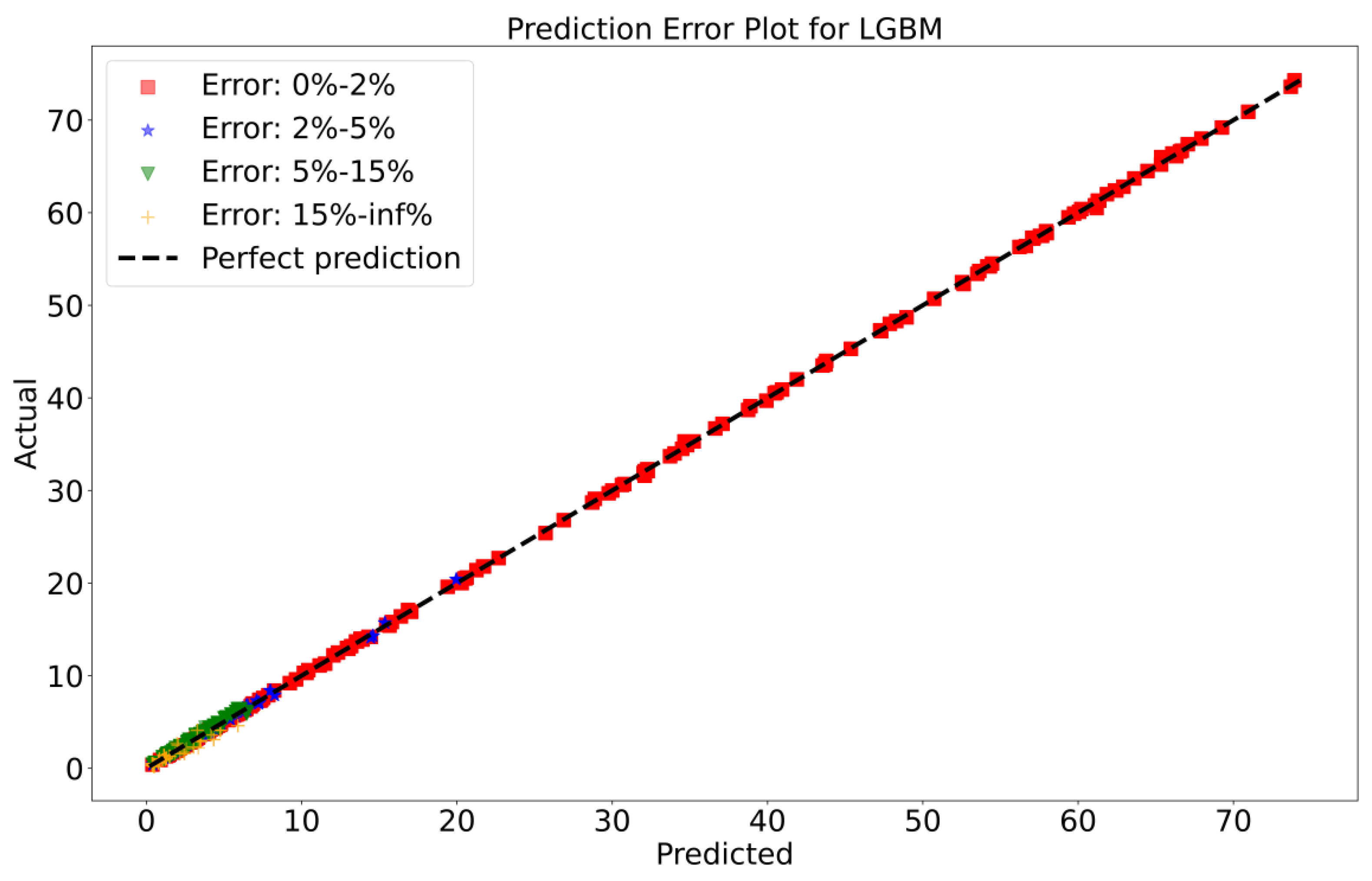
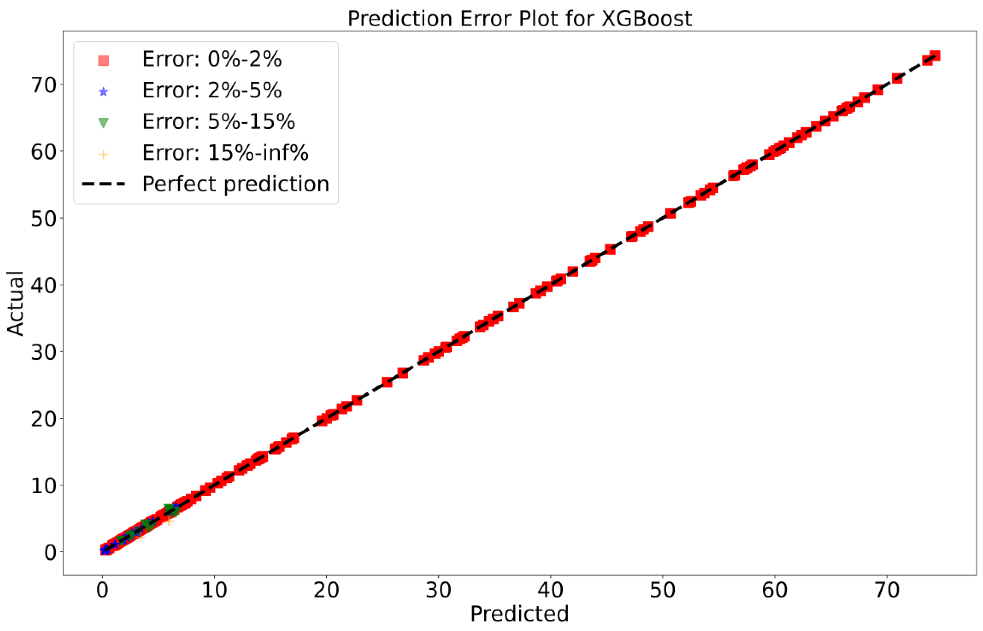
To attain a better understanding of CatBoost, LGBM, XGBoost, and Lasso, error scatter plots (shown in Figure 15, Figure 16, Figure 17 and Figure 18) were developed to highlight the link between predicted and actual rainfall for CatBoost, LGBM, XGBoost, and Lasso. An investigation of these figures suggests that a data point error of less than 0 to 2% has been recorded. In comparison with XGBoost, LGBM has a higher rate of data point errors, ranging from 2% to 15% for the rainfall dataset. Similarly, with CatBoost, data point errors range from 5 to 10% for the rainfall dataset; however, very little error was noticed for the XGBoost between these points. Lasso shows the highest percentage of data point errors, with values greater than 15% for rainfall data. Taking all these aspects into account, it is fair to say that the XGBoost model outperformed both CatBoost and LGBM in terms of robustness and dependability for weekly rainfall predictions.
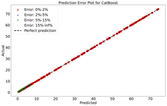
Figure 15.
Scatter plots of rainfall forecasting for the CatBoost Model-2.
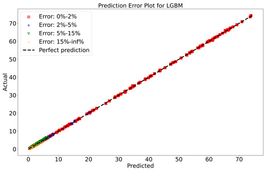
Figure 16.
Scatter plots of rainfall forecasting for the LGBM Model-2.
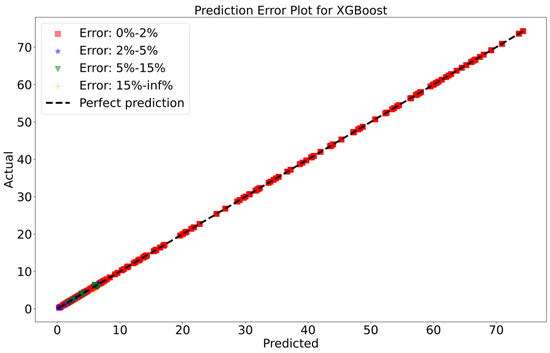
Figure 17.
Scatter plots of rainfall forecasting for the XGBoost Model-2.
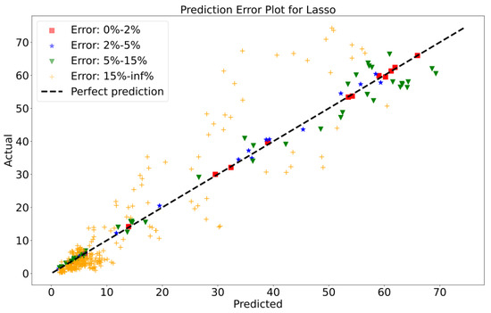
Figure 18.
Scatter plots of rainfall forecasting for the Lasso Model-2.
CatBoost demonstrated effective handling of categorical characteristics while also being resistant to overfitting. XGBoost provided versatility in handling diverse data formats and provided useful feature significance scores. LightGBM stood out for its efficiency in training speed and memory utilization, making it suited for larger datasets. In contrast, linear regression-based models such as Lasso and Ridge provided interpretability and simplicity. However, these linear models may struggle to capture complicated non-linear patterns in these data and are vulnerable to outliers.
6. Conclusions
CatBoost consistently emerged as the best-performing model in all evaluation stages, including training, validation, and testing, for Model-1. Its accuracy, as seen by low MAE, MSE, RMSE, RMSPE, and high R2 scores, demonstrated its ability to capture this dataset’s unique temporal patterns. Furthermore, XGBoost and LGBM performed admirably; however, they fell slightly short of CatBoost. In Model-2, XGBoost outperformed other methods with remarkable accuracy and continuously low error rates. The ability of this model to effectively capture weekly rainfall patterns demonstrated its appropriateness for predicting longer time intervals. The ensemble-based algorithms, particularly CatBoost and XGBoost, outperformed standard linear regression-based methods (Lasso, Ridge, and Linear Regression) and LGBM in both models. The scatter plots demonstrated CatBoost and XGBoost’s superiority in maintaining a low percentage of prediction errors across the dataset. The findings of this work highlight the importance of ensemble approaches, particularly CatBoost and XGBoost, in reliable rainfall prediction for major cities. To advance predictive efficacy, future avenues of research could entail the incorporation of supplementary variables, finer temporal segmentation for enhanced granularity, and the exploration of advanced feature engineering techniques.
Author Contributions
Conceptualization, V.K. and K.V.S.; methodology, V.K. and N.K.; Investigation, K.M.K. and A.E.A.; resources, K.M.K. and A.E.A.; writing—original draft preparation, V.K. and K.V.S.; writing—review and editing, K.M.K. and A.E.A.; supervision, V.K.; project administration, N.K. All authors have read and agreed to the published version of the manuscript.
Funding
This research work was supported by the Deanship of Scientific Research at King Khalid University under grant number RGP. 2/422/44.
Institutional Review Board Statement
Not applicable.
Informed Consent Statement
Not applicable.
Data Availability Statement
For direct interaction with our best trained CatBoost rainfall prediction model, please visit the dedicated web application at https://rainfallpredictiondelhi.streamlit.app/.
Acknowledgments
The Authors extend their appreciation to the Deanship Scientific Research at King Khalid University for funding this work through a large group. Project group number RGP. 2/422/44.
Conflicts of Interest
The authors declare no conflict of interest.
References
- Rayner, S.; Lach, D.; Ingram, H. Weather Forecasts are for Wimps: Why Water Resource Managers Do Not Use Climate Forecasts. Clim. Chang. 2005, 69, 197–227. [Google Scholar] [CrossRef]
- Toth, E.; Brath, A.; Montanari, A. Comparison of short-term rainfall prediction models for real-time flood forecasting. J. Hydrol. 2000, 239, 132–147. [Google Scholar] [CrossRef]
- Park, J.; Seager, T.P.; Rao, P.S.C.; Convertino, M.; Linkov, I. Integrating Risk and Resilience Approaches to Catastrophe Management in Engineering Systems. Risk Anal. 2013, 33, 356–367. [Google Scholar] [CrossRef] [PubMed]
- Funk, C.C.; Brown, M.E. Declining global per capita agricultural production and warming oceans threaten food security. Food Secur. 2009, 1, 271–289. [Google Scholar] [CrossRef]
- Lagouvardos, K.; Kotroni, V.; Bezes, A.; Koletsis, I.; Kopania, T.; Lykoudis, S.; Mazarakis, N.; Papagiannaki, K.; Vougioukas, S. The automatic weather stations NOANN network of the National Observatory of Athens: Operation and database. Geosci. Data J. 2017, 4, 4–16. [Google Scholar] [CrossRef]
- Yuan, Q.; Shen, H.; Li, T.; Li, Z.; Li, S.; Jiang, Y.; Xu, H.; Tan, W.; Yang, Q.; Wang, J.; et al. Deep learning in environmental remote sensing: Achievements and challenges. Remote Sens. Environ. 2020, 241, 111716. [Google Scholar] [CrossRef]
- Kumar, V.; Yadav, S.M. Real-Time Flood Analysis Using Artificial Neural Network. In Recent Trends in Civil Engineering; Pathak, K.K., Bandara, J.M.S.J., Agrawal, R., Eds.; Lecture Notes in Civil Engineering; Springer: Singapore, 2021; Volume 77, pp. 973–986. [Google Scholar] [CrossRef]
- Kumar, V.; Yadav, S.M. A state-of-the-Art review of heuristic and metaheuristic optimization techniques for the management of water resources. Water Supply 2022, 22, 3702–3728. [Google Scholar] [CrossRef]
- McNeill, I.M.; Dunlop, P.D.; Heath, J.B.; Skinner, T.C.; Morrison, D.L. Expecting the Unexpected: Predicting Physiological and Psychological Wildfire Preparedness from Perceived Risk, Responsibility, and Obstacles. Risk Anal. 2013, 33, 1829–1843. [Google Scholar] [CrossRef]
- Fletcher, T.D.; Andrieu, H.; Hamel, P. Understanding, management and modelling of urban hydrology and its consequences for receiving waters: A state of the art. Adv. Water Resour. 2013, 51, 261–279. [Google Scholar] [CrossRef]
- Ming, X.; Liang, Q.; Xia, X.; Li, D.; Fowler, H.J. Real-Time Flood Forecasting Based on a High-Performance 2-D Hydrodynamic Model and Numerical Weather Predictions. Water Resour. Res. 2020, 56, e2019WR025583. [Google Scholar] [CrossRef]
- Debortoli, N.S.; Camarinha, P.I.M.; Marengo, J.A.; Rodrigues, R.R. An index of Brazil’s vulnerability to expected increases in natural flash flooding and landslide disasters in the context of climate change. Nat. Hazards 2017, 86, 557–582. [Google Scholar] [CrossRef]
- Glade, T. Applying Probability Determination to Refine Landslide-triggering Rainfall Thresholds Using an Empirical. Pure Appl. Geophys. 2000, 157, 1059–1079. [Google Scholar] [CrossRef]
- He, X.; Guan, H.; Zhang, X.; Simmons, C.T. A wavelet-based multiple linear regression model for forecasting monthly rainfall. Int. J. Climatol. 2014, 34, 1898–1912. [Google Scholar] [CrossRef]
- Swain, S.; Patel, P.; Nandi, S. A multiple linear regression model for precipitation forecasting over Cuttack district, Odisha, India. In Proceedings of the 2017 2nd International Conference for Convergence in Technology (I2CT), Pune, India, 8–9 April 2017; pp. 355–357. [Google Scholar]
- Choubin, B.; Khalighi-Sigaroodi, S.; Malekian, A.; Kişi, Ö. Multiple linear regression, multi-layer perceptron network and adaptive neuro-fuzzy inference system for forecasting precipitation based on large-scale climate signals. Hydrol. Sci. J. 2016, 61, 1001–1009. [Google Scholar] [CrossRef]
- Bostan, P.A.; Heuvelink, G.B.M.; Akyurek, S.Z. Comparison of regression and kriging techniques for mapping the average annual precipitation of Turkey. Int. J. Appl. Earth Obs. Geoinf. 2012, 19, 115–126. [Google Scholar] [CrossRef]
- He, C.; Wei, J.; Song, Y.; Luo, J.-J. Seasonal Prediction of Summer Precipitation in the Middle and Lower Reaches of the Yangtze River Valley: Comparison of Machine Learning and Climate Model Predictions. Water 2021, 13, 3294. [Google Scholar] [CrossRef]
- Cappelli, F.; Conigliani, C.; Consoli, D.; Costantini, V.; Paglialunga, E. Climate change and armed conflicts in Africa: Temporal persistence, non-linear climate impact and geographical spillovers. Econ. Polit. 2023, 40, 517–560. [Google Scholar] [CrossRef]
- Pour, S.H.; Wahab, A.K.A.; Shahid, S. Physical-empirical models for prediction of seasonal rainfall extremes of Peninsular Malaysia. Atmos. Res. 2020, 233, 104720. [Google Scholar] [CrossRef]
- Diop, L.; Samadianfard, S.; Bodian, A.; Yaseen, Z.M.; Ghorbani, M.A.; Salimi, H. Annual Rainfall Forecasting Using Hybrid Artificial Intelligence Model: Integration of Multilayer Perceptron with Whale Optimization Algorithm. Water Resour. Manag. 2020, 34, 733–746. [Google Scholar] [CrossRef]
- Luk, K.C.; Ball, J.E.; Sharma, A. An application of artificial neural networks for rainfall forecasting. Math. Comput. Model. 2001, 33, 683–693. [Google Scholar] [CrossRef]
- Abbot, J.; Marohasy, J. Input selection and optimisation for monthly rainfall forecasting in Queensland, Australia, using artificial neural networks. Atmos. Res. 2014, 138, 166–178. [Google Scholar] [CrossRef]
- Hong, W.-C. Rainfall forecasting by technological machine learning models. Appl. Math. Comput. 2008, 200, 41–57. [Google Scholar] [CrossRef]
- Karamouz, M.; Razavi, S.; Araghinejad, S. Long-lead seasonal rainfall forecasting using time-delay recurrent neural networks: A case study. Hydrol. Process. 2008, 22, 229–241. [Google Scholar] [CrossRef]
- Bojang, P.O.; Yang, T.-C.; Pham, Q.B.; Yu, P.-S. Linking Singular Spectrum Analysis and Machine Learning for Monthly Rainfall Forecasting. Appl. Sci. 2020, 10, 3224. [Google Scholar] [CrossRef]
- Das, P.; Sachindra, D.A.; Chanda, K. Machine Learning-Based Rainfall Forecasting with Multiple Non-Linear Feature Selection Algorithms. Water Resour. Manag. 2022, 36, 6043–6071. [Google Scholar] [CrossRef]
- Monego, V.S.; Anochi, J.A.; de Campos Velho, H.F. South America Seasonal Precipitation Prediction by Gradient-Boosting Machine-Learning Approach. Atmosphere 2022, 13, 243. [Google Scholar] [CrossRef]
- Appiah-Badu, N.K.A.; Missah, Y.M.; Amekudzi, L.K.; Ussiph, N.; Frimpong, T.; Ahene, E. Rainfall Prediction Using Machine Learning Algorithms for the Various Ecological Zones of Ghana. IEEE Access 2022, 10, 5069–5082. [Google Scholar] [CrossRef]
- Jamei, M.; Ali, M.; Malik, A.; Karbasi, M.; Rai, P.; Yaseen, Z.M. Development of a TVF-EMD-based multi-decomposition technique integrated with Encoder-Decoder-Bidirectional-LSTM for monthly rainfall forecasting. J. Hydrol. 2023, 617, 129105. [Google Scholar] [CrossRef]
- Ali, M.; Prasad, R.; Xiang, Y.; Yaseen, Z.M. Complete ensemble empirical mode decomposition hybridized with random forest and kernel ridge regression model for monthly rainfall forecasts. J. Hydrol. 2020, 584, 124647. [Google Scholar] [CrossRef]
- Gigović, L.; Pourghasemi, H.R.; Drobnjak, S.; Bai, S. Testing a New Ensemble Model Based on SVM and Random Forest in Forest Fire Susceptibility Assessment and Its Mapping in Serbia’s Tara National Park. Forests 2019, 10, 408. [Google Scholar] [CrossRef]
- Yu, P.-S.; Yang, T.-C.; Chen, S.-Y.; Kuo, C.-M.; Tseng, H.-W. Comparison of random forests and support vector machine for real-time radar-derived rainfall forecasting. J. Hydrol. 2017, 552, 92–104. [Google Scholar] [CrossRef]
- Singh, K.; Singh, B.; Sihag, P.; Kumar, V.; Sharma, K.V. Development and application of modeling techniques to estimate the unsaturated hydraulic conductivity. Model. Earth Syst. Environ. 2023, in press. [Google Scholar] [CrossRef]
- Ghorbani, M.A.; Khatibi, R.; Karimi, V.; Yaseen, Z.M.; Zounemat-Kermani, M. Learning from Multiple Models Using Artificial Intelligence to Improve Model Prediction Accuracies: Application to River Flows. Water Resour. Manag. 2018, 32, 4201–4215. [Google Scholar] [CrossRef]
- Kisi, O.; Choubin, B.; Deo, R.C.; Yaseen, Z.M. Incorporating synoptic-scale climate signals for streamflow modelling over the Mediterranean region using machine learning models. Hydrol. Sci. J. 2019, 64, 1240–1252. [Google Scholar] [CrossRef]
- Kumar, V.; Azamathulla, H.M.; Sharma, K.V.; Mehta, D.J.; Maharaj, K.T. The State of the Art in Deep Learning Applications, Challenges, and Future Prospects: A Comprehensive Review of Flood Forecasting and Management. Sustainability 2023, 15, 10543. [Google Scholar] [CrossRef]
- Liang, Z.; Li, Y.; Hu, Y.; Li, B.; Wang, J. A data-driven SVR model for long-term runoff prediction and uncertainty analysis based on the Bayesian framework. Theor. Appl. Climatol. 2018, 133, 137–149. [Google Scholar] [CrossRef]
- Kamir, E.; Waldner, F.; Hochman, Z. Estimating wheat yields in Australia using climate records, satellite image time series and machine learning methods. ISPRS J. Photogramm. Remote Sens. 2020, 160, 124–135. [Google Scholar] [CrossRef]
- Kumar, V.; Sharma, K.V.; Caloiero, T.; Mehta, D.J.; Singh, K. Comprehensive Overview of Flood Modeling Approaches: A Review of Recent Advances. Hydrology 2023, 10, 141. [Google Scholar] [CrossRef]
- Chen, C.; Zhang, Q.; Kashani, M.H.; Jun, C.; Bateni, S.M.; Band, S.S.; Dash, S.S.; Chau, K.-W. Forecast of rainfall distribution based on fixed sliding window long short-term memory. Eng. Appl. Comput. Fluid Mech. 2022, 16, 248–261. [Google Scholar] [CrossRef]
- Haq, D.Z.; Rini Novitasari, D.C.; Hamid, A.; Ulinnuha, N.; Arnita; Farida, Y.; Nugraheni, R.D.; Nariswari, R.; Ilham; Rohayani, H.; et al. Long Short-Term Memory Algorithm for Rainfall Prediction Based on El-Nino and IOD Data. Procedia Comput. Sci. 2021, 179, 829–837. [Google Scholar] [CrossRef]
- Elsayed, S.; Gupta, M.; Chaudhary, G.; Taneja, S.; Gaur, H.; Gad, M.; Hamdy Eid, M.; Kovács, A.; Péter, S.; Gaagai, A.; et al. Interpretation the Influence of Hydrometeorological Variables on Soil Temperature Prediction Using the Potential of Deep Learning Model. Knowl. Based Eng. Sci. 2023, 4, 55–77. [Google Scholar] [CrossRef]
- Zhao, J.; Gao, Y.; Qu, Y.; Yin, H.; Liu, Y.; Sun, H. Travel Time Prediction: Based on Gated Recurrent Unit Method and Data Fusion. IEEE Access 2018, 6, 70463–70472. [Google Scholar] [CrossRef]
- Haidar, A.; Verma, B. Monthly Rainfall Forecasting Using One-Dimensional Deep Convolutional Neural Network. IEEE Access 2018, 6, 69053–69063. [Google Scholar] [CrossRef]
- Chong, K.L.; Lai, S.H.; Yao, Y.; Ahmed, A.N.; Jaafar, W.Z.W.; El-Shafie, A. Performance Enhancement Model for Rainfall Forecasting Utilizing Integrated Wavelet-Convolutional Neural Network. Water Resour. Manag. 2020, 34, 2371–2387. [Google Scholar] [CrossRef]
- Li, W.; Pan, B.; Xia, J.; Duan, Q. Convolutional neural network-based statistical post-processing of ensemble precipitation forecasts. J. Hydrol. 2022, 605, 127301. [Google Scholar] [CrossRef]
- Sahin, E.K. Assessing the predictive capability of ensemble tree methods for landslide susceptibility mapping using XGBoost, gradient boosting machine, and random forest. SN Appl. Sci. 2020, 2, 1308. [Google Scholar] [CrossRef]
- Malik, A.; Saggi, M.K.; Rehman, S.; Sajjad, H.; Inyurt, S.; Bhatia, A.S.; Farooque, A.A.; Oudah, A.Y.; Yaseen, Z.M. Deep learning versus gradient boosting machine for pan evaporation prediction. Eng. Appl. Comput. Fluid Mech. 2022, 16, 570–587. [Google Scholar] [CrossRef]
- Alves Basilio, S.; Goliatt, L. Gradient Boosting Hybridized with Exponential Natural Evolution Strategies for Estimating the Strength of Geopolymer Self-Compacting Concrete. Knowl. Based Eng. Sci. 2022, 3, 1–16. [Google Scholar] [CrossRef]
- Xenochristou, M.; Hutton, C.; Hofman, J.; Kapelan, Z. Water Demand Forecasting Accuracy and Influencing Factors at Different Spatial Scales Using a Gradient Boosting Machine. Water Resour. Res. 2020, 56, e2019WR026304. [Google Scholar] [CrossRef]
- Naganna, S.R.; Beyaztas, B.H.; Bokde, N.; Armanuos, A.M. On the evaluation of the gradient tree boosting model for groundwater level forecasting. Knowl. Based Eng. Sci. 2020, 1, 48–57. [Google Scholar] [CrossRef]
- Dong, J.; Zeng, W.; Wu, L.; Huang, J.; Gaiser, T.; Srivastava, A.K. Enhancing short-term forecasting of daily precipitation using numerical weather prediction bias correcting with XGBoost in different regions of China. Eng. Appl. Artif. Intell. 2023, 117, 105579. [Google Scholar] [CrossRef]
- Sanders, W.; Li, D.; Li, W.; Fang, Z.N. Data-Driven Flood Alert System (FAS) Using Extreme Gradient Boosting (XGBoost) to Forecast Flood Stages. Water 2022, 14, 747. [Google Scholar] [CrossRef]
- Ghanim, A.A.J.; Shaf, A.; Ali, T.; Zafar, M.; Al-Areeq, A.M.; Alyami, S.H.; Irfan, M.; Rahman, S. An Improved Flood Susceptibility Assessment in Jeddah, Saudi Arabia, Using Advanced Machine Learning Techniques. Water 2023, 15, 2511. [Google Scholar] [CrossRef]
- Seireg, H.R.; Omar, Y.M.K.; El-Samie, F.E.A.; El-Fishawy, A.S.; Elmahalawy, A. Ensemble Machine Learning Techniques Using Computer Simulation Data for Wild Blueberry Yield Prediction. IEEE Access 2022, 10, 64671–64687. [Google Scholar] [CrossRef]
- Diao, L.; Niu, D.; Zang, Z.; Chen, C. Short-term Weather Forecast Based on Wavelet Denoising and Catboost. In Proceedings of the 2019 Chinese Control Conference (CCC), Guangzhou, China, 27–30 July 2019; IEEE: New York, NY, USA; pp. 3760–3764. [Google Scholar]
- Karbasi, M.; Jamei, M.; Ali, M.; Abdulla, S.; Chu, X.; Yaseen, Z.M. Developing a novel hybrid Auto Encoder Decoder Bidirectional Gated Recurrent Unit model enhanced with empirical wavelet transform and Boruta-Catboost to forecast significant wave height. J. Clean. Prod. 2022, 379, 134820. [Google Scholar] [CrossRef]
- Shahriar, S.A.; Kayes, I.; Hasan, K.; Hasan, M.; Islam, R.; Awang, N.R.; Hamzah, Z.; Rak, A.E.; Salam, M.A. Potential of ARIMA-ANN, ARIMA-SVM, DT and CatBoost for Atmospheric PM2.5 Forecasting in Bangladesh. Atmosphere 2021, 12, 100. [Google Scholar] [CrossRef]
- Budhiraja, B.; Gawuc, L.; Agrawal, G. Seasonality of Surface Urban Heat Island in Delhi City Region Measured by Local Climate Zones and Conventional Indicators. IEEE J. Sel. Top. Appl. Earth Obs. Remote Sens. 2019, 12, 5223–5232. [Google Scholar] [CrossRef]
- Dutta, D.; Rahman, A.; Paul, S.K.; Kundu, A. Impervious surface growth and its inter-relationship with vegetation cover and land surface temperature in peri-urban areas of Delhi. Urban Clim. 2021, 37, 100799. [Google Scholar] [CrossRef]
- Gurjar, B.R.; Jain, A.; Sharma, A.; Agarwal, A.; Gupta, P.; Nagpure, A.S.; Lelieveld, J. Human health risks in megacities due to air pollution. Atmos. Environ. 2010, 44, 4606–4613. [Google Scholar] [CrossRef]
- Bickici Arikan, B.; Jiechen, L.; Sabbah, I.I.D.; Ewees, A.; Homsi, R.; Sulaiman, S.O. Dew Point Time Series Forecasting at the North Dakota. Knowl. Based Eng. Sci. 2021, 2, 24–34. [Google Scholar] [CrossRef]
- Kumar, V.; Kedam, N.; Sharma, K.V.; Mehta, D.J.; Caloiero, T. Advanced Machine Learning Techniques to Improve Hydrological Prediction: A Comparative Analysis of Streamflow Prediction Models. Water 2023, 15, 2572. [Google Scholar] [CrossRef]
- Fan, J.; Ma, X.; Wu, L.; Zhang, F.; Yu, X.; Zeng, W. Light Gradient Boosting Machine: An efficient soft computing model for estimating daily reference evapotranspiration with local and external meteorological data. Agric. Water Manag. 2019, 225, 105758. [Google Scholar] [CrossRef]
- Sheridan, R.P.; Wang, W.M.; Liaw, A.; Ma, J.; Gifford, E.M. Extreme Gradient Boosting as a Method for Quantitative Structure–Activity Relationships. J. Chem. Inf. Model. 2016, 56, 2353–2360. [Google Scholar] [CrossRef]
- Prokhorenkova, L.; Gusev, G.; Vorobev, A.; Dorogush, A.V.; Gulin, A. Catboost: Unbiased boosting with categorical features. In Advances in Neural Information Processing Systems; Bengio, S., Wallach, H., Larochelle, H., Grauman, K., Cesa-Bianchi, N., Garnett, R., Eds.; Curran Associates, Inc.: New York, NY, USA, 2018; Volume 31, pp. 6638–6648. [Google Scholar]
- Luo, X.; Chang, X.; Ban, X. Regression and classification using extreme learning machine based on L1-norm and L2-norm. Neurocomputing 2016, 174, 179–186. [Google Scholar] [CrossRef]
- McDonald, G.C. Ridge regression. Wiley Interdiscip. Rev. Comput. Stat. 2009, 1, 93–100. [Google Scholar] [CrossRef]
- Su, X.; Yan, X.; Tsai, C.-L. Linear regression. Wiley Interdiscip. Rev. Comput. Stat. 2012, 4, 275–294. [Google Scholar] [CrossRef]


Disclaimer/Publisher’s Note: The statements, opinions and data contained in all publications are solely those of the individual author(s) and contributor(s) and not of MDPI and/or the editor(s). MDPI and/or the editor(s) disclaim responsibility for any injury to people or property resulting from any ideas, methods, instructions or products referred to in the content. |
© 2023 by the authors. Licensee MDPI, Basel, Switzerland. This article is an open access article distributed under the terms and conditions of the Creative Commons Attribution (CC BY) license (https://creativecommons.org/licenses/by/4.0/).