Machine Learning Assessment of Damage Grade for Post-Earthquake Buildings: A Three-Stage Approach Directly Handling Categorical Features

Abstract

The rapid assessment of post-earthquake building damage for rescue and reconstruction is a crucial strategy to reduce the enormous number of human casualties and economic losses caused by earthquakes. Conventional machine learning (ML) approaches for this problem usually employ one-hot encoding to cope with categorical features, and their overall procedure is neither sufficient nor comprehensive. Therefore, this study proposed a three-stage approach, which can directly handle categorical features and enhance the entire methodology of ML applications. In stage I, an integrated data preprocessing framework involving subjective–objective feature selection was proposed and performed on a dataset of buildings after the 2015 Gorkha earthquake. In stage II, four machine learning models, KNN, XGBoost, CatBoost, and LightGBM, were trained and tested on the dataset. The best model was judged by comprehensive metrics, including the proposed risk coefficient. In stage III, the feature importance, the relationships between the features and the model’s output, and the feature interaction effects were investigated by Shapley additive explanations. The results indicate that the LightGBM model has the best overall performance with the highest accuracy of 0.897, the lowest risk coefficient of 0.042, and the shortest training time of 12.68 s due to its relevant algorithms for directly tackling categorical features. As for its interpretability, the most important features are determined, and information on these features’ impacts and interactions is obtained to improve the reliability of and promote practical engineering applications for the ML models. The proposed three-stage approach can provide a reference for the overall ML implementation process on raw datasets for similar problems.

1. Introduction

In recent years, earthquake disasters have resulted in an enormous number of casualties and economic losses [1,2,3]. In 2010, Haiti was severely impacted by an earthquake with a moment magnitude (M_w) of 7 which left 316,000 people dead or missing, millions of people homeless, and more than half of the buildings around the epicenter damaged [4]. In 2015, an earthquake with an M_w of 7.8 struck Gorkha, Nepal, resulting in over 30,000 people dead or injured, eight million people displaced, 500,000 houses destroyed, and another 250,000 houses damaged [5]. In 2023, a 7.8 M_w earthquake happened in Turkey and Syria, where there were around 55,000 fatalities, 130,000 injuries, and 50,000 destroyed or badly damaged structures as a result of the tragedy, which affected approximately 18 million people [6,7]. Given the above shocking and alarming facts, it would be useful to be able to rapidly identify buildings with severe and light damage after an earthquake to implement proper rescue and reconstruction, facilitating the sustainable development of cities.

Some conventional assessment techniques have been developed based on empirical principles. Ningthoujam and Nanda proposed a robust and straightforward approach to evaluating the safety of concrete buildings against earthquakes in India, considering features such as whether the buildings are soft story, their age, whether they have substantial overhang, and so on [8]. Khan et al. employed a rapid visual screening approach of FEMA P-154 to assess the seismic vulnerability of existing buildings in Malakand, a region with an elevated risk [9]. Diana et al. predicted displacement demand and building damage grades (DGs) more accurately by typological capacity curves and the modified N2 method for Nordic countries [10]. Ozer et al. developed a comprehensive framework to assess seismic damage efficiently and accurately in multi-story buildings. This framework operates in near real time and encompasses three distinct levels of analysis: an empirical formulation, the effective stiffness concept, and the finite element model [11]. Martínez-Cuevas et al. performed statistical modeling and found discrimination metrics based on various national criteria and a ranking of features to assess the habitability of houses after earthquakes [12].

Machine learning (ML) is another favorable approach to address the subjectivity underlying empirical formulas and consider the potential impact of a broader range of features. Chaurasia et al. performed predictions using a neural network and the random forest model, and the best-performing model’s F1 score was 0.743. [13]. Chen and Zhang used a cloud model and Bayesian networks to predict the DG in three levels with an accuracy of 0.888 based on a dataset of 9920 buildings [14]. A year later, they performed a three-grade damage prediction by ensemble learning with an accuracy of 0.783 based on a dataset of 12,045 buildings [15]. K.C. et al. trained and tested four ML models to predict building damage in five grades for 549,251 buildings and found that XGBoost had the highest accuracy of 0.577 [16].

It is acknowledged that ML can achieve high-accuracy damage grade assessments; however, it is typically realized by complex models, many of which are black boxes that are challenging even for experts to interpret [17]. Moreover, erroneous decisions that arise from the models may have severe repercussions, necessitating interpretability methods to guarantee the reliability of the decisions. Feature importance offers a simplified and global interpretation by ranking the importance of the features [18]. Partial dependence plots and accumulated local effects plots can present the average impact of features on predictions, and the latter has a broader range of applications as it is free from the limitation of the feature independence assumption [19,20]. Shapely additive explanations stem from game theory and elucidate the importance of features by comparing the mean change in model output through the presence or absence of features after constructing combinations of different features [21,22].

In the above studies, conventional empirical assessment techniques incorporate empirical formulations that are constrained by the researchers’ experience and that have limited regional applicability. In addition, the limited considered features make it challenging to capture the potential feature influence and gain deeper insight into the mechanism in complex scenarios. Consequently, ML assessment approaches are preferred. However, when the ML models were implemented in the above studies, there was inadequate attention given to data preprocessing, affecting the accuracy and efficiency of the ML models. Additionally, none of them directly dealt with categorical features but employed one-hot encoding, increasing the feature dimensions and computational cost. Moreover, there was not enough consideration of the reliability the models when applied to practical engineering projects.

To bridge this gap, this paper proposed a three-stage approach, which can directly handle categorical features and achieve high-accuracy damage grade assessments of post-earthquake buildings. Meanwhile, the proposed approach enhanced the entire problem-solving methodology, i.e., before, during, and after the implementation of the ML models, to improve the models’ accuracy and reliability. The remaining sections of the paper are organized as follows. In Section 2, the fundamental concepts and principles underlying the utilized ML models, evaluation metrics, and interpretability method are reviewed. In Section 3, the implementation of the three-stage approach is described in detail, including data preprocessing, the development of the ML models, and the development of the interpretability method for the best-performing model. In Section 4, the primary findings and limitations of the study are provided, and potential avenues for further research are presented.

2. Overview of Machine Learning and Interpretability Methods

2.1. Machine Learning Methods

2.1.1. K-Nearest Neighbors (KNNs)

The KNN algorithm is a non-parametric and supervised model, classifying samples relying on their closest neighbor’s majority vote [23]. KNNs are influenced by the predominant number of samples among the closest K points, which, in turn, determines the quantity of neighbors K in the final result [24,25]. The distance metrics can be determined by various functions, among which the Heterogeneous Euclidean-Overlap Metric (HEOM) is suggested, as presented in Equation (1) [26]:

$$d\left(X,Y\right)=\sqrt{{\displaystyle \sum _{n=1}^m{d}_n\left(x_n-y_n\right)}}$$

(1)

where $d_n\left(x_n-y_n\right)$ denotes the distance between two observed samples in the nth feature.

A KNN is easy to implement and adapts easily, but it does not scale well and is prone to overfitting. The KNN algorithm works on the following principles [27]:

(1)

Determine the distance between each training and test set of data;

(2)

Sort by the increasing distance;

(3)

Choose the K points with the shortest distance;

(4)

Determine the frequency of occurrence of the category in which the first K points belong;

(5)

Provide the data class that appears the most frequently in the first K points as the classification result of the test data.

2.1.2. Extreme Gradient Boosting (XGBoost)

In ML techniques, extreme gradient boosting is an algorithm for ensemble learning, commonly called XGBoost [28]. It integrates statistical boosting approaches and contains classification and regression trees (CARTs) that are pretty straightforward. Boosting is a technique that improves a model’s accuracy by building several trees rather than a single tree and then combining those trees into a single prediction framework. This helps refine the estimation precision by increasing the model’s accuracy [29]. XGBoost constructs the tree by iteratively utilizing the residuals from the previous trees as contributions to the resulting tree. Consequently, the resulting tree evolves by capturing the accumulated errors of the previous trees, ultimately refining the overall prediction. The growth of the new tree ceases either upon reaching the predetermined maximum limit of trees or when the training error fails to improve over a specified quantity of successive trees. Including random sampling in gradient boosting significantly improves the accuracy of estimations and the speed of execution. This integrated technique, probabilistic boosting, enhances the algorithm’s overall performance [30]. The objective function of XGBoost consists of a loss function and a penalty term, as presented in Equation (2) [31,32]:

$$Ob{j}^{\left(t\right)}={\displaystyle \sum _{i}l\left(y_i,{\widehat{y}}_i^{\left(t\right)}\right)}+{\displaystyle \sum _k\Omega \left(f_k\right)}$$

(2)

where t represents the tth iteration of training; l quantifies the difference between the actual value and the predicted value; and $\Omega \left(f_k\right)=\gamma T+\frac{1}{2}\lambda {\Vert \omega \Vert }^2$ is the penalty term governing the complexity of the kth tree [33]. In the penalty term, $\gamma$ and $\lambda$ represent the complexity of the leaves and the penalty parameter. T and ${\Vert \omega \Vert }^2$ denote the leaf count and the output of each leaf node [34]. Further details of the XGBoost model can be found in the studies [35,36,37].

2.1.3. Categorical Boosting (CatBoost)

CatBoost, an unbiased gradient boosting algorithm, handles categorical features directly [38]. Its notable characteristics include the capability to deal with categorical features and the novel order-boosting method without predicting shifts. It offers distinct solutions for various categorical features. CatBoost optimizes its tree splitting process instead of preprocessing. The features contain a limited number of classes, so the classifier incorporates one-hot encoding to transform the categorical features into numeric representations based on their frequency. As for combined features, the classes are substituted with the mean target value. This feature transformation will signify the loss of information regarding the interplay between categorical features. Therefore, CatBoost considers the prior amalgamation of the characteristics of the present state alongside the remaining categorical features. CatBoost can decrease model overfitting using the feature conversion value, as presented in Equation (3) [39,40]:

$${\widehat{x}}_i^k=\frac{{\displaystyle \sum _{j=1}^n\phi \left(x_j^k=x_i^k\right)Y_j}+\alpha p}{{\displaystyle \sum _{j=1}^n\phi \left(x_j^k=x_i^k\right)+\alpha }}$$

(3)

where $x_i^k$ and $x_j^k$ are the kth feature vectors in the ith and jth sample groups, respectively, and i and j fall within the range of 1 to n (the number of the sample groups); $\phi , Y_j, \alpha , \mathrm{and} p$ are the indicator function, ith target value, prior weight, and prior value, respectively.

The Minimal Variance Sampling (MVS) training mechanism is also a highlight of CatBoost. MVS is a weighted sampling variant of the regularization sampling technology. CatBoost incorporates all the settings needed to build separate decision trees and set up the random forest. The literature [41,42,43] can be referenced for further information about CatBoost.

2.1.4. Light Gradient Boosting Machine (LightGBM)

LightGBM is an exceptionally efficient implementation of the gradient boosting decision tree (GBDT) algorithm [44]. Unlike the traditional approach of level-wise tree growth, LightGBM adopts a leaf-wise growth approach for its decision trees, which are displayed in Figure 1a,b, respectively. The level-wise growth approach splits leaves on the identical layer simultaneously, assisting in model complexity controlling and multi-threading optimization. It processes all leaves in the same layer without distinction, increasing superfluous calculations and inefficiency. The leaf-wise growth approach, however, only selects and splits the leaf with the highest information gain each time. The information gain is calculated as follows [45,46]:

$$IG\left(A,W\right)=En\left(A\right)-{\displaystyle \sum _{w\in Values\left(W\right)}\frac{\left|A_w\right|}{A}En\left(A_w\right)}$$

(4)

$$En\left(A\right)={\displaystyle \sum _{d=1}^D-p_d{\log }_2{p}_d}$$

(5)

where En (A) and En (A_w) are the information entropy of the collection A and its subset A_w whose feature value is w, respectively; w, D, and p_d are the value of feature W, the number of categories, and the ratio of A to category d, respectively. Though the leaf-wise approach can assist in reducing errors and achieving greater accuracy, it may lead to overfitting due to the growth of a pretty deep decision tree, necessitating a maximum depth constraint.

Figure 1c displays how the characteristics are binned, and the histogram approach is employed. Additionally, Gradient-based One-Side Sampling (GOSS) reduces training samples, while Exclusive Feature Bundling (EFB) merges features. The GOSS method assumes that samples with greater gradients affect information gain more than those with lower gradients. GOSS first sorts samples by their gradient absolute value in decreasing order. Next, a part of the top samples is chosen. GOSS also picks a fraction of the remaining data for sampling. EFB views characteristics as vertices and clashes as weighted edges, grouping them as graph colors. GOSS and EFB reduce computational complexity without affecting accuracy. LightGBM has a high accuracy, fast training speed, efficient handling of big data, and GPU-accelerated learning. Details of the LightGBM are provided in the literature [47,48,49].

2.2. Machine Learning Evaluation Metrics

Accuracy, precision, and recall are three common fundamental metrics. These metrics are formally defined by true positive (TP), false negative (FN), false positive (FP), and true negative (TN), as illustrated in Figure 2.

Accuracy, an overall metric that evaluates the performance of all categories, is defined by the proportion of correctly predicted samples, i.e., TP and TN, to the total number, as presented in Equation (6). The classification performance of a specific category can be evaluated by precision and recall. Precision is the truly predicted proportion of the predicted positive, and recall is the proportion that is successfully predicted as positive in the actual positive, which are defined in Equations (7) and (8).

$$\mathrm{Accuracy}=\frac{\mathrm{TP}+\mathrm{TN}}{\mathrm{TP}+\mathrm{TN}+\mathrm{FP}+\mathrm{FN}}$$

(6)

$$\mathrm{Precicsion}=\frac{\mathrm{TP}}{\mathrm{TP}+\mathrm{FP}}$$

(7)

$$\mathrm{Recall}=\frac{\mathrm{TP}}{\mathrm{TP}+\mathrm{FN}}$$

(8)

The confusion matrix is a visualized approach to assessing the performance of ML classification models. The classification of the three DGs in this study is represented by a confusion matrix consisting of three rows and three columns, as demonstrated in Figure 3.

From Figure 3, the element on the pth row and qth column is N_{p, q}, representing the number of samples that are predicted as the pth category and actually belong to the qth category. The elements on the main diagonal are true positives, and the depth of blue indicates their sizes. Other elements are misclassified samples, including true negatives, false positives, and false negatives, and the depth of orange indicates their sizes. The confusion matrix provides a clear view of how the categories are predicted and confused in the classification. Meanwhile, it can also be used to calculate accuracy, precision, and recall.

Reliability is essential for models that may be applied to practical engineering projects. In this problem, misclassifying a high DG as a low DG leads to considerable risk. To quantitatively assess this risk, it is supposed that damage resulting from the misclassification of DG as 3 to 2 and 2 to 1 is set to 1, and the damage caused by the misclassification of DG as 3 to 1 is set to 2. Then, a novel metric risk coefficient is proposed, which can be defined as follows:

$$\mathrm{Risk} \mathrm{coefficient}=\frac{N_{3,2}+N_{2,1}+2N_{3,1}}{{\displaystyle \sum _{p=1}^3{\displaystyle \sum _{q=1}^3{N}_{p,q}}}}$$

(9)

The smaller the risk coefficient, the less potential damage the model may cause due to misclassification.

Moreover, the training time should also be taken into consideration. In practical applications, the number of samples involved in training can be numerous, while the time available for training is limited since the relevant people need to race against time to save victims and reinforce buildings after an earthquake. At this time, the shorter the training time, the better the model is. It can be implemented with the time library, which is a Python native library and does not require an additional download.

2.3. Interpretability Method: Shapely Additive Explanations

The Shapely Additive Explanations (SHAP) framework was introduced by Lundberg and Lee, drawing inspiration from game theory and local explanations. This methodology offers a promising approach to interpreting ML models [21,22]. As defined by SHAP, the explanation for a model with m input features is represented by a linear function g consisting of m binary features as follows:

$$g\left(z\right)={\phi }_0+{\displaystyle \sum _{i=1}^m{\phi }_i{z_i}^{\prime }}$$

(10)

where ${z_i}^{\prime }$ is 1 when a feature is observed; otherwise, it is 0. ${\phi }_0$ represents the base value of the prediction, and ${\phi }_i$ denotes the contribution of the ith feature.

The calculation of the contribution of the ith feature, referred to as the SHAP value, is performed using the conditional output of subsets derived from game theory:

$${\phi }_i={\displaystyle \sum _{S\in M\left\{i\right\}}\frac{\left|S\right|!\left(M-S-1\right)!}{M!}\left[f_x\left(S\cup \left\{i\right\}\right)-f_x\left(S\right)\right]}$$

(11)

where M is the set of m features; S denotes all feature subsets that exclude the ith feature; the output of a tree when considering a specific feature subset S is $f_x\left(S\right)=\left[E\left(f\left(x\right)|x_s\right)\right]$; and $f_x\left(S\cup \left\{i\right\}\right)$ and $f_x\left(i\right)$ are the expected output of models that include and exclude the ith feature, respectively. A comprehensive explanation of SHAP can be referred to in the literature [50].

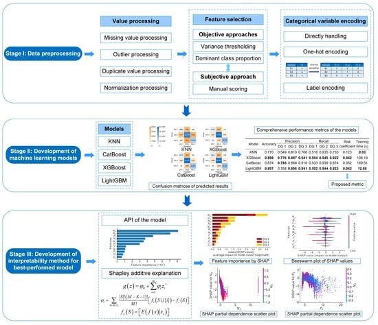
3. Modeling of Damage Grade Assessment for Buildings

On 25 April 2015 at 11:56 AM NPT (UTC+5:45), an earthquake occurred in Gorkha, Nepal, as presented in Figure 4 [51]. The magnitude was 7.8. The location of the epicenter was 28.15° N and 84.71° E, and the depth was 15.0 km. Furthermore, there were three significant aftershocks with magnitudes of about 7. The first two occurred on the 25th and 26th of April, while the other happened on the 12th of May. More than 600,000 structures in Kathmandu and its surrounding areas experienced varying degrees of damage or destruction. Additionally, a considerable loss of human life occurred, with a reported death toll of approximately 9000 individuals. This seismic event was experienced throughout Nepal’s central and eastern regions, a significant portion of the Ganges River valley in India’s northern part, the northwestern area of Bangladesh, the southern plateau of Tibet, and the western region of Bhutan [51].

In 2016, Kathmandu Living Labs and the Central Bureau of Statistics conducted a comprehensive household survey utilizing mobile technology. The effects of the earthquake, the state of households, and demographic and economic data were all covered in this survey. The dataset utilized in this study was acquired from a comprehensive dataset and subsequently streamlined to align with the research goals of this paper, as documented by Driven Data [52]. The dataset consists of 214,839 rows and 39 columns. In this context, it can be observed that each row within the given dataset corresponds to a distinct building, while each column represents a specific feature associated with these buildings. Three distinct grades of damage exist, namely one, two, and three, which correspond to minimal damage, moderate damage, and near-total devastation, respectively.

3.1. Stage I: Data Preprocessing

First, an integrated data preprocessing framework was proposed, including missing value processing, outlier processing, duplicate value processing, normalization processing, feature selection, and variable encoding [53]. The whole process is shown in Figure 5.

3.1.1. Missing Value Processing

Missing values can occur for several reasons, such as the unsuccessful acquisition of data, an accident while storing or transferring data, etc. First, for a building, if more than half of its 39 features have missing values, then this row of data should be discarded directly. If not, training after filling in the missing values may affect the model’s accuracy. Then, owing to the categorical features in the dataset, linear interpolation and cubic spline interpolation filling methods are not appropriate. The missing value is filled with the nearest non-missing value in that column of data. If the two non-missing values closest to the missing value are equal in distance to it, then one is randomly chosen to fill the missing value.

3.1.2. Outlier Processing

Outliers can also occur in the dataset, perhaps due to the wrong information being obtained while acquiring, storing, or transferring data. It is noted that there are three types of data in the dataset: int, categorical, and binary, and the possible values are specified. Thus, if a value in the column is outside the specified range, it is considered an outlier. Here, the range is determined by the median absolute deviation algorithm [53]. Similarly, if more than half of a building’s feature data are outliers, the building’s data should be discarded. The replacement of outliers was performed using a method similar to the missing value filling method, i.e., replacing an outlier with the nearest non-outlier in that column.

3.1.3. Duplicate Value Processing

Duplicate values appearing in the variable building_id need to be handled. Because the values of the building_id variable represent the unique identification of a building, two buildings cannot have the same value. The building_id variable is first tabulated and sorted in descending order. For building_id variables with occurrences greater than 1, the row with fewer missing values and outliers is kept; otherwise, the front row is kept.

3.1.4. Normalization Processing

Since the dimensions and specific ranges of features are different, normalization is required to speed up the training of ML models and may improve accuracy. The normalization method is min–max normalization realized by the MinMaxScaler function of the sklearn library [54]. It should be noted that only int-type variables are processed here, binary variables are not processed, and categorical variables are processed in subsequent steps.

3.1.5. Feature Selection

There are 39 features in the dataset, which is quite a lot. Thus, the features need to be selected to accelerate the training and prediction of the model. Before that, it is noted that the variables associated with has_superstructure and has_secondary_use are all binary variables, which can be turned into categorical variables to reduce the number of features and compact the information expression. Afterwards, 19 features are able to express the information expressed by the original 39 features. Furthermore, the building_id feature is removed because it only serves to distinguish each building and does not substantially contribute to the judgment of DG. Information on the remaining 18 features is shown in

Table 1. The building features after preprocessing for ML modeling.

Feature	Identifier	Type	Description	Possible Values
geo_level_1_id	Ng1	int	from broadest (level 1) to narrowest (level 3) in terms of the building’s geographical location	0–30
geo_level_2_id	Ng2			0–1427
geo_level_3_id	Ng3			0–12,567
count_floors_pre_eq	Nfl		post-earthquake number of floors of the building	no exact value range
age	Na		number of years the building has been in existence	no exact value range
count_families	Nfa		number of family members residing in the building	0–9
area_percentage	Pa		normalized area of the building footprint	no exact value range
height_percentage	Ph		normalized height of the building footprint	no exact value range
land_surface_condition	Cls	categorical	the surface condition of the land for the location of the building	n, o, t.
foundation_type	Tf		foundation type of the building	h, i, r, u, w.
roof_type	Tr		roof type of the building	n, q, x.
ground_floor_type	Tg		ground floor type of the building	f, m, v, x, z.
other_floor_type	To		type of constructions utilized for stories above ground level (other than the roof)	j, q, s, x.
position	Pb		position of the building	j, o, s, t.
plan_configuration	Cp		building plan configuration	a, c, d, f, m, n, o, q, s, u.
has_superstructure	Css		the material of the superstructure	am, b, cmb, cms, mmb, mms, o, rce, rcne, sf, t
legal_ownership_status	Clos		legal ownership status of the land for the location of the building	a, r, v, w.
has_secondary_use	Csu		whether the building is being used secondarily and what its specific purpose is	a, go, h, hp, ind, ins, no, o, r, s, up

.

In Table 1, the specific meanings of the classes for C_ss are am (adobe/mud), b (bamboo), cmb (cement mortar–brick), cms (cement mortar–stone), mmb (mud mortar–brick), mms (mud mortar–stone), o (other materials), rce (engineered reinforced concrete), rcne (non-engineered reinforced concrete), sf (stone), and t (timber). Additionally, the specific meanings of the classes for C_su are a (agricultural purposes), go (government office), h (hotel), hp (health post), ind (industrial purposes), ins (institution), no (no secondary use), o (other purposes), r (rental purposes), s (school), and up (police station). Further details about the features and classes are provided in the literature [55].

During the feature selection, a combination of objective and subjective methods was employed. The variance thresholding method was used for the objective feature selection method, which is effective only for int-type features. The variance along with the min, max, and standard deviation of the features for reference are presented in

Table 2. The statistical description of int-type features.

Feature	Ng1	Ng2	Ng3	Nfl	Na	Pa	Ph	Nfa
Min	0	0	0	1	0	1	2	0
Max	30	1427	12,567	9	995	100	32	9
Standard deviation	8.07	413.05	3661.10	0.73	75.65	4.52	1.95	0.42
Variance	65.08	170,606.27	13,403,651.08	0.54	5723.67	20.47	3.82	0.18

The bolded ones are the variance values less than 1, and the corresponding features are considered for elimination.

.

For categorical features, since the variance cannot be calculated, according to a similar idea of variance thresholding, the dominant class proportion, i.e., the proportion of the class with the largest number to the total number (214,839) in the features, was used as the criterion. The calculation results are shown in

Table 3. The proportion of the class with the largest number to the total number in the features.

Feature	Cls	Tf	Tr	Tg	To	Pb	Cp	Css	Clos	Csu
Proportion	0.83	0.83	0.69	0.80	0.63	0.77	0.96	0.72	0.96	0.89

Similarly, the values greater than 0.8 are bolded, and their corresponding features are given consideration for elimination.

.

For the subjective feature selection method, manual scoring was conducted here, primarily considering their potential contribution to the DG in terms of the physical significance of the features. The scoring range is from 0 to 1, and the results are displayed in

Table 4. Manual scoring considering the contribution of features based on physical significance.

Feature	Ng1	Ng2	Ng3	Nfl	Na	Pa	Ph	Nfa	Cls
Score	1	1	1	0.8	0.8	0.7	0.7	0.3	0.8
Feature	Tf	Tr	Tg	To	Pb	Cp	Css	Clos	Csu
Score	0.7	0.5	0.7	0.4	0.6	0.6	0.7	0.4	0.3

The bolded values are less than 0.5, and the corresponding features are deemed to be eliminated.

.

For a comprehensive evaluation, the information in the above three tables was considered simultaneously. The features with bolded values for their variance (or proportion) and score, i.e., N_fa, T_o, C_los, and C_su, were directly eliminated. For T_f, T_g, and C_p, although their scores are greater than 0.5, they are all less than or equal to 0.7. Furthermore, they provide less information because their proportion is over 0.8, so they were also eliminated. For N_fl and C_ls with bolded values for their variance (or proportion), their scores are both 0.8, revealing that they are essential and should be retained.

Therefore, the retained features are N_g1, N_g2, N_g3, N_fl, N_a, P_a, P_h, C_ls, T_r, P_b, and C_ss.

3.1.6. Categorical Variable Encoding

Among the selected models, KNN and XGBoost do not support categorical features, while CatBoost and LightGBM do. For the data to be trained in KNN and XGBoost, one-hot encoding is required, which can be implemented by the get_dummies function of the pandas library [56]. The process of one-hot encoding is illustrated in Figure 6. A categorical feature with N_c specific categories can be transformed into N_c binary variables with 0 and 1 representing whether it belongs to a category or not. For a sample, only one of these binary variables is 1, and the rest are 0. The binary variables are guaranteed to be equidistant for each category, unlike directly mapping specific categories to integers 0, 1, …, N_c−1, which are non-equidistant. However, this method results in a rise in dimensions, which can be particularly significant when N_c is large, thus greatly increasing the training and prediction time of the model.

Similarly, apart from features in the KNN and XGBoost, the training labels also need to be encoded, but one-hot encoding cannot be employed here. Instead, they are directly mapped to integers from 0 to N_L−1, where N_L−1 is the number of categories of the label, which is named label encoding.

3.2. Stage II: Development of the Machine Learning Models

First, the data were visualized to exhibit the distribution of DG on the relationship plot between the features. Since there are categorical features, the pairplot function of the seaborn library is not appropriate. Hence, the function scatterplot was utilized [57]. The plots were completed in the following order: N_g1, N_g2, N_g3, N_fl, N_a, P_a, P_h, C_ls, T_r, P_b, and C_ss. For a certain feature, its relationships with the next-to-last features were plotted to ensure orderliness and non-repetition. For the visualization of DG, the damage severity increases from 1 to 3 and is represented in orange, red, and dark red with different shapes, respectively, indicating the increasing severity. Due to the excessive amount of data, 500 samples were randomly selected for plotting, and the relationships between the features with DGs are displayed in Figure 7.

From Figure 7, abundant information can be obtained. For instance, from the third-to-last subfigure in Figure 7, it is found that for (Tr, Pb), the DG tends to be one when it is (x, o), (x, t), or (x, s). When it is (n, o), (n, s), (q, j), (q, t), or (x, j), the DG is generally two. When it is (n, j), (n, t), or (q, s), the DG is more prone to be three. Preliminarily understanding the influence of the relationship between the features on the DG can help establish a general and comprehensive view of the data.

Subsequently, four ML models, KNN, XGBoost, CatBoost, and LightGBM, were selected and developed. The KNN was selected because of its straightforward concept and few hyperparameters. Then, three ensemble learning algorithms, XGBoost, CatBoost, and LightGBM, were chosen due to their typically superior performance. These four algorithms can be divided into two groups for a subsequent comparison and discussion: the KNN and XGBoost cannot directly handle categorical features, whereas CatBoost and LightGBM can. The environment is Anaconda 3 and python 3.10.4. The primarily utilized libraries are sklearn 1.1.2, lightgbm 3.3.2, xgboost 1.6.2, catboost 1.2, shap 0.41.0, numpy 1.23.1, and pandas 1.4.3. For splitting the dataset, seventy percent was allocated as the training dataset, while the remaining thirty percent was designated as the test dataset. Preliminary training was performed using the default hyperparameters of the model as a baseline, and then hyperparameters tuning was performed using GridSearchCV, setting a five-fold cross-validation [54]. The model’s accuracy with the default and optimal hyperparameters are provided in

Table 5. Model accuracy with default and optimal hyperparameters.

Model	Accuracy				Detailed Optimal Hyperparameters
	Default Hyperparameters		Optimal Hyperparameters
	Training Set	Test Set	Training Set	Test Set
KNN	0.841	0.770	0.876	0.770	n_neighbors = 3
XGBoost	0.877	0.861	0.969	0.898	learning_rate = 0.1, n_estimators = 1200, min_child_weight = 1, gamma = 0, max_depth = 8
CatBoost	0.858	0.849	0.908	0.874	depth = 8, learning_rate = 0.15, iterations = 1200
LightGBM	0.840	0.835	0.975	0.897	learning_rate = 0.1, n_estimators = 1200, num_leaves = 100, max_depth = 8, colsample_bytree = 0.8, subsample = 0.8

.

From Table 5, with the assistance of GridSearchCV, the optimal hyperparameters of the model were found, and the accuracy of the training and test datasets of all the models except the KNN was improved considerably.

After obtaining the optimal hyperparameters, the models were trained and tested, and their performance could be intuitively grasped and analyzed through the confusion matrices. The elements on the main diagonal or other positions are true positives or misclassified samples, whose sizes are indicated by the depth of blue or orange, respectively. The confusion matrices of the predicted DGs for the models of the training dataset are displayed in Figure 8.

Based on the findings presented in Figure 8, it can be discerned that the KNN model exhibited the least favorable performance for the training set, whereas the LightGBM model demonstrated the most optimal performance. The XGBoost model exhibits a marginally inferior performance compared to the LightGBM model, yet it remains highly advantageous. The performance of the CatBoost model is moderate, particularly when evaluating the 6384 samples with a DG of 1 as 2. This misjudgment stands out as the most significant among the four models.

Figure 9 presents the confusion matrices depicting the predicted DGs of the models for the test dataset.

From Figure 9, it is indicated that for the test set, the KNN model still performed the worst, while the LightGBM and XGBoost models performed comparably, both being the best. For the CatBoost model, the number of samples misclassifying the DG as 1 instead of 2 is roughly the same as that of the KNN model, revealing that the misclassification has improved, though the overall performance remains moderate.

Next, the models with optimal hyperparameters were evaluated by comprehensive metrics, including accuracy, precision, recall, the proposed risk coefficient, and the training time, as presented in

Table 6. Performance metrics of the models with optimal hyperparameters on the test dataset (except training time on the training dataset).

Model	Accuracy	Precision			Recall			Risk Coefficient	Training Time (s)
		DG 1	DG 2	DG 3	DG 1	DG 2	DG 3
KNN	0.770	0.549	0.810	0.766	0.516	0.835	0.733	0.123	0.03
XGBoost	0.898	0.776	0.897	0.941	0.594	0.945	0.922	0.042	108.19
CatBoost	0.874	0.785	0.868	0.916	0.533	0.939	0.874	0.052	169.51
LightGBM	0.897	0.768	0.896	0.941	0.592	0.944	0.923	0.042	12.68

The top two values of each metric are bolded to emphasize the two best performances [58].

and Figure 10.

As displayed in Table 6, the training time of the KNN model is the shortest, only 0.03 s, but none of its other metrics are in the top two. Thus, this model may be applied to a specific scenario with limited training time. For the CatBoost model, the precision of DG 1 reaches a high level. However, its general performance in other aspects makes it less appropriate for DG assessments. The XGBoost and LightGBM models performed fairly well, with eight out of nine metrics in the top two. To further compare the discrepancy between their parameters, the training time of the LightGBM model is 12.68 s, which is considerably smaller than the 108.19 s of the XGBoost model. Moreover, the precision of DG 1 of the LightGBM model is 0.768, slightly smaller than that of the XGBoost model (0.776).

Therefore, from Table 6 and Figure 10, the LightGBM model is regarded as the best-performing model for DG assessments in this paper after a comprehensive evaluation. The accuracy is 0.897, which is satisfactory compared to the studies of Chen and Zhang [14,15], with reported accuracies of 0.888 and 0.783.

3.3. Stage III: Development of the Interpretability Method for the Best-Performing Model

To enhance the comprehension of the model operation mechanism and ensure the safety of the application for practical engineering, the best-performing model, i.e., the LightGBM model, was interpreted by its application programming interface (API), as displayed in Figure 11.

From Figure 11, the five most important features are N_g3, N_g2, P_a, N_a, and N_g1, indicating that the DG is closely connected with the buildings’ locations, ages, and normalized footprint areas.

Then, the model was interpreted by SHAP. A global comprehension of the feature importance for different DGs can be implemented by visualizing the mean absolute SHAP value of the features, which is illustrated in Figure 12.

From Figure 12, the features N_g1, N_g2, and N_g3, which are related to the geographical locations, are essential, occupying three of the five most essential features. C_ss indicates the materials of the superstructures. The strength and stiffness of construction materials vary greatly, resulting in different levels of resistance to earthquakes, so C_ss is also crucial. N_a, the age of the buildings in years, is also vital. The aging of the buildings over time leads to a decrease in the load-bearing capacity of their components, thus increasing seismic damage. For DG 1, the three most prominent features are N_g1, N_a, and C_ss. For DG 2, they are N_g1, N_g2, and N_g3. For DG 3, they are N_g1, C_ss, and N_g2. They are generally similar but locally different.

Compared with Figure 11, both emphasize the importance of location and age. Summarizing the perspectives of the model API and SHAP, the six most important metrics are N_g2, N_g1, N_g3, N_a, P_a, and C_ss. Other features also have undeniable contributions to the model, but not as much as these previous features.

To investigate how the features impact the output of the LightGBM model, Figure 13 provides an information-dense summary. From Figure 13a, the SHAP values increase as N_a, N_fl, and P_h decrease, revealing a positive impact on DG 1 judgments. The effect becomes compounded for N_g1, N_g2, N_g3, and P_a, and their increase may have a positive or negative impact on DG 1’s judgments. It is comprehensible since the features N_g1, N_g2, and N_g3, which are associated with geographic locations, are artificially defined, and their magnitudes do not have a high physical significance. As C_ss, T_r, C_ls, and P_b are categorical variables, no size difference exists between specific categories. Hence, they are presented in gray and are not discussed here.

From Figure 13b, with the increase in P_a and N_fl, the SHAP value rises, thus positively impacting DG 2 judgments. Similarly, the effects of N_g1, N_g2, and N_g3 on DG 2 judgments are also compounded. Interestingly, for P_h and N_a, their reduction brings the SHAP value to nearly 0, revealing slight effects. In contrast, an elevation in P_h and N_a levels would lead to an SHAP value that is either positive or negative, indicating a potentially heightened positive or negative influence. By conducting a comparable analysis, as shown in Figure 13c, one can also deduce the influence of the variation in features on the judgment of DG 3.

Combining the information from the three figures yields the integrated impact of the features on the three DG judgments. Taking N_a as an example, Figure 13a,c illustrate that as N_a rises, the trends for the SHAP value are exactly the opposite. In Figure 13b, when the values of N_a are low, the SHAP values are close to 0. Furthermore, the increase in N_a gives rise to both positive and negative SHAP values. Therefore, it can be concluded that a newly constructed building tends to be judged as DG 1. When a building is older, it may be more likely to be judged as DG 2 or 3.

Furthermore, apart from illustrating the impact of the variation in a singular feature on the model output in Figure 13, SHAP can also demonstrate the interaction effects of the features, as depicted in Figure 14. Taking Figure 14a as an example, the SHAP values for the same value of N_g1 are distinct, revealing nonlinear interaction effects between the two features of N_g1 and N_fl. Otherwise, there will be no vertical dispersion in the figure, and the scatter points will ideally obey the line determined by the dependence_plot function. Figure 14c shows that the interaction effects between N_a and N_fl are particularly prominent. When the values of N_a are close to 0, the scatter points are predominantly blue, suggesting that the current values of N_fl are low, and the corresponding SHAP values are more than 0, indicating a positive impact on the model’s output. However, most scatter points become red as N_a rises from 0 to 3. At this time, the values of N_fl are larger, and the corresponding SHAP values are nearly less than 0, reflecting a negative impact. Figure 14i shows that when T_r is n or x, with the increase in N_fl, the SHAP value gradually changes from negative to 0 and then to positive, signifying that the impact on the model’s output progressively varies from negative to positive. When T_r equals q, the values of N_fl are typically greater, and the SHAP value may be positive or negative, implying a weak interaction.

The results and discussion in this stage provide a more informative and compact interpretation of the best-performing model compared to previous similar studies [15,16,59]. By directly coping with categorical features rather than employing one-hot encoding, information fragmentation attributed to transforming a categorical feature into several binary features is prevented. The proposed approach can comprehend the impact of features on the model’s output and reflect the interaction effects between features involving categorical features, thereby enhancing the model’s reliability. Simultaneously, a greater understanding of these models can also guide data acquisition to determine the features to be considered.

4. Conclusions

This paper employed a three-stage framework including four ML models, a series of evaluation metrics, and an interpretability method. In stage I, data preprocessing and feature selection were conducted on a dataset of the buildings after the 2015 Gorkha earthquake. In stage II, four ML models were trained and tested on the selected dataset to determine the best-performing model. In stage III, the best-performing model was interpreted to exhibit the feature importance and the relationships between the input and output variables. The conclusions can be summarized as follows.

(1)

An integrated data preprocessing framework combined with subjective–objective feature selection was proposed to accelerate the model training and prediction without losing an excessive amount of accuracy, providing a reference for similar problems.

(2)

The LightGBM and CatBoost models directly handle categorical features with training times of 12.68 s and 169.51 s, while the XGBoost model tackles features by one-hot encoding with a training time of 108.19 s. Given the guarantee of accuracy, the algorithms in LightGBM for handling categorical features can significantly accelerate training, while those in CatBoost instead increase the training time for this problem.

(3)

The LightGBM and XGBoost models have the highest accuracies of 0.897 and 0.898, followed by the CatBoost model with 0.874. The KNN model may be less appropriate for this problem, with an accuracy of only 0.770.

(4)

The risk coefficient was proposed to evaluate the safety of the model classification quantitatively, and the risk coefficients of the KNN, XGBoost, CatBoost, and LightGBM models were 0.123, 0.042, 0.052, and 0.042. The safety of the XGBoost and LightGBM models was the highest.

(5)

Comparing the accuracy, precision, recall, risk coefficient, and training time of the four models, the LightGBM model has the best overall performance.

(6)

To visualize the mechanism of the LightGBM model by its API and SHAP, the six most essential features are N_g2, N_g1, N_g3, N_a, P_a, and C_ss. The impact of N_g1, N_g2, and N_g3 variations on the model output are all compound, while that of other features is related to the specific damage grade, presenting a monotonic or compound influence.

Nevertheless, this research is subject to some limitations. It only focused on features regarding buildings and their environments. Meanwhile, current interpretability approaches are inadequate for categorical features. For instance, beeswarm plots of SHAP values of features are incompatible with categorical features.

Therefore, future work can consider the features of seismic waves or other aspects to improve the accuracy and expand the range of potential applications. Moreover, more advanced interpretability techniques for categorical features should be developed and utilized to ensure the reliability and robustness of the models for practical engineering applications.

References

1. Cariolet, J.-M.; Vuillet, M.; Diab, Y. Mapping Urban Resilience to Disasters—A Review. Sustain. Cities Soc. 2019, 51, 101746. [Google Scholar] [CrossRef]
2. Han, L.; Ma, Q.; Zhang, F.; Zhang, Y.; Zhang, J.; Bao, Y.; Zhao, J. Risk Assessment of An Earthquake-Collapse-Landslide Disaster Chain by Bayesian Network and Newmark Models. Int. J. Environ. Res. Public. Health 2019, 16, 3330. [Google Scholar] [CrossRef] [PubMed]
3. Qiang, Y.; Huang, Q.; Xu, J. Observing Community Resilience from Space: Using Nighttime Lights to Model Economic Disturbance and Recovery Pattern in Natural Disaster. Sustain. Cities Soc. 2020, 57, 102115. [Google Scholar] [CrossRef]
4. DesRoches, R.; Comerio, M.; Eberhard, M.; Mooney, W.; Rix, G.J. Overview of the 2010 Haiti Earthquake. Earthq. Spectra 2011, 27, 1–21. [Google Scholar] [CrossRef]
5. Chaulagain, H.; Gautam, D.; Rodrigues, H. Chapter 1—Revisiting Major Historical Earthquakes in Nepal: Overview of 1833, 1934, 1980, 1988, 2011, and 2015 Seismic Events. In Impacts and Insights of the Gorkha Earthquake; Gautam, D., Rodrigues, H., Eds.; Elsevier: Amsterdam, The Netherlands, 2018; pp. 1–17. ISBN 978-0-12-812808-4. [Google Scholar]
6. Chen, W.; Rao, G.; Kang, D.; Wan, Z.; Wang, D. Early Report of the Source Characteristics, Ground Motions, and Casualty Estimates of the 2023 Mw 7.8 and 7.5 Turkey Earthquakes. J. Earth Sci. 2023, 34, 297–303. [Google Scholar] [CrossRef]
7. Omer, S. 2023 Turkey and Syria Earthquake: Facts, FAQs, and How to Help. Available online: https://www.worldvision.org/disaster-relief-news-stories/2023-turkey-and-syria-earthquake-faqs (accessed on 6 June 2023).
8. Ningthoujam, M.C.; Nanda, R.P. A GIS System Integrated with Earthquake Vulnerability Assessment of RC Building. Structures 2018, 15, 329–340. [Google Scholar] [CrossRef]
9. Khan, S.U.; Qureshi, M.I.; Rana, I.A.; Maqsoom, A. Seismic Vulnerability Assessment of Building Stock of Malakand (Pakistan) Using FEMA P-154 Method. SN Appl. Sci. 2019, 1, 1625. [Google Scholar] [CrossRef]
10. Diana, L.; Lestuzzi, P.; Podestà, S.; Luchini, C. Improved Urban Seismic Vulnerability Assessment Using Typological Curves and Accurate Displacement Demand Prediction. J. Earthq. Eng. 2021, 25, 1709–1731. [Google Scholar] [CrossRef]
11. Ozer, E.; Özcebe, A.G.; Negulescu, C.; Kharazian, A.; Borzi, B.; Bozzoni, F.; Molina, S.; Peloso, S.; Tubaldi, E. Vibration-Based and Near Real-Time Seismic Damage Assessment Adaptive to Building Knowledge Level. Buildings 2022, 12, 416. [Google Scholar] [CrossRef]
12. Martínez-Cuevas, S.; Morillo Balsera, M.C.; Benito, B.; Torres, Y.; Gaspar-Escribano, J.; Staller, A.; García-Aranda, C. Assessing Building Habitability after an Earthquake Using Building Typology and Damage Grade. Application in Lorca, Spain. J. Earthq. Eng. 2022, 26, 3417–3439. [Google Scholar] [CrossRef]
13. Chaurasia, K.; Kanse, S.; Yewale, A.; Singh, V.K.; Sharma, B.; Dattu, B.R. Predicting Damage to Buildings Caused by Earthquakes Using Machine Learning Techniques. In Proceedings of the 2019 IEEE 9th International Conference on Advanced Computing (IACC 2019), Tiruchirappalli, India, 13–14 December 2019; IEEE: New York, NY, USA, 2019; pp. 81–86. [Google Scholar]
14. Chen, W.; Zhang, L. Predicting Building Damages in Mega-Disasters under Uncertainty: An Improved Bayesian Network Learning Approach. Sustain. Cities Soc. 2021, 66, 102689. [Google Scholar] [CrossRef]
15. Chen, W.; Zhang, L. Building Vulnerability Assessment in Seismic Areas Using Ensemble Learning: A Nepal Case Study. J. Clean. Prod. 2022, 350, 131418. [Google Scholar] [CrossRef]
16. Sajan, K.C.; Bhusal, A.; Gautam, D.; Rupakhety, R. Earthquake Damage and Rehabilitation Intervention Prediction Using Machine Learning. Eng. Fail. Anal. 2023, 144, 106949. [Google Scholar] [CrossRef]
17. Zio, E. Prognostics and Health Management (PHM): Where Are We and Where Do We (Need to) Go in Theory and Practice. Reliab. Eng. Syst. Saf. 2022, 218, 108119. [Google Scholar] [CrossRef]
18. Wei, P.; Lu, Z.; Song, J. Variable Importance Analysis: A Comprehensive Review. Reliab. Eng. Syst. Saf. 2015, 142, 399–432. [Google Scholar] [CrossRef]
19. Friedman, J.H. Greedy Function Approximation: A Gradient Boosting Machine. Ann. Stat. 2001, 29, 1189–1232. [Google Scholar] [CrossRef]
20. Apley, D.W.; Zhu, J. Visualizing the Effects of Predictor Variables in Black Box Supervised Learning Models. arXiv 2019, arXiv:1612.08468. [Google Scholar] [CrossRef]
21. Lundberg, S.M.; Lee, S.-I. A Unified Approach to Interpreting Model Predictions. In Proceedings of the Advances in Neural Information Processing Systems, Long Beach, CA, USA, 4–9 December 2017; Curran Associates, Inc.: New York, NY, USA, 2017; Volume 30. [Google Scholar]
22. Lundberg, S.M.; Erion, G.G.; Lee, S.-I. Consistent Individualized Feature Attribution for Tree Ensembles. arXiv 2019, arXiv:1802.03888. [Google Scholar]
23. Bangyal, W.H.; Qasim, R.; Rehman, N.U.; Ahmad, Z.; Dar, H.; Rukhsar, L.; Aman, Z.; Ahmad, J. Detection of Fake News Text Classification on COVID-19 Using Deep Learning Approaches. Comput. Math. Methods Med. 2021, 2021, 5514220. [Google Scholar] [CrossRef]
24. Zhang, S.; Li, X.; Zong, M.; Zhu, X.; Cheng, D. Learning k for KNN Classification. ACM Trans. Intell. Syst. Technol. 2017, 8, 1–19. [Google Scholar] [CrossRef]
25. Zhang, S.; Li, X.; Zong, M.; Zhu, X.; Wang, R. Efficient KNN Classification With Different Numbers of Nearest Neighbors. IEEE Trans. Neural Netw. Learn. Syst. 2018, 29, 1774–1785. [Google Scholar] [CrossRef] [PubMed]
26. Salvador–Meneses, J.; Ruiz–Chavez, Z.; Garcia–Rodriguez, J. Compressed KNN: K-Nearest Neighbors with Data Compression. Entropy 2019, 21, 234. [Google Scholar] [CrossRef] [PubMed]
27. Guo, G.; Wang, H.; Bell, D.; Bi, Y.; Greer, K. KNN Model-Based Approach in Classification. In Proceedings of the On The Move to Meaningful Internet Systems 2003: CoopIS, DOA, and ODBASE, Sicily, Italy, 3–7 November 2003; Meersman, R., Tari, Z., Schmidt, D.C., Eds.; Springer: Berlin/Heidelberg, Germany, 2003; pp. 986–996. [Google Scholar]
28. Chen, T.; Guestrin, C. XGBoost: A Scalable Tree Boosting System. In Proceedings of the 22nd ACM SIGKDD International Conference on Knowledge Discovery and Data Mining, San Francisco, CA, USA, 13 August 2016; Association for Computing Machinery: New York, NY, USA, 2016; pp. 785–794. [Google Scholar]
29. Elith, J.; Leathwick, J.R.; Hastie, T. A Working Guide to Boosted Regression Trees. J. Anim. Ecol. 2008, 77, 802–813. [Google Scholar] [CrossRef] [PubMed]
30. Friedman, J.H. Stochastic Gradient Boosting. Comput. Stat. Data Anal. 2002, 38, 367–378. [Google Scholar] [CrossRef]
31. Fatahi, R.; Nasiri, H.; Homafar, A.; Khosravi, R.; Siavoshi, H.; Chelgani, S. Modeling Operational Cement Rotary Kiln Variables with Explainable Artificial Intelligence Methods—A “Conscious Lab” Development. Part. Sci. Technol. 2022, 41, 715–724. [Google Scholar] [CrossRef]
32. Le, T.-T.-H.; Oktian, Y.; Kim, H. XGBoost for Imbalanced Multiclass Classification-Based Industrial Internet of Things Intrusion Detection Systems. Sustainability 2022, 14, 8707. [Google Scholar] [CrossRef]
33. Nasiri, H.; Alavi, S.A. A Novel Framework Based on Deep Learning and ANOVA Feature Selection Method for Diagnosis of COVID-19 Cases from Chest X-Ray Images. Comput. Intell. Neurosci. 2022, 2022, e4694567. [Google Scholar] [CrossRef]
34. Fatahi, R.; Nasiri, H.; Dadfar, E.; Chelgani, S. Modeling of Energy Consumption Factors for an Industrial Cement Vertical Roller Mill by SHAP-XGBoost: A “Conscious Lab” Approach. Sci. Rep. 2022, 12, 7543. [Google Scholar] [CrossRef]
35. Alajmi, M.S.; Almeshal, A.M. Predicting the Tool Wear of a Drilling Process Using Novel Machine Learning XGBoost-SDA. Materials 2020, 13, 4952. [Google Scholar] [CrossRef]
36. Wan, Z.; Xu, Y.; Šavija, B. On the Use of Machine Learning Models for Prediction of Compressive Strength of Concrete: Influence of Dimensionality Reduction on the Model Performance. Materials 2021, 14, 713. [Google Scholar] [CrossRef]
37. Xu, B.; Tan, Y.; Sun, W.; Ma, T.; Liu, H.; Wang, D. Study on the Prediction of the Uniaxial Compressive Strength of Rock Based on the SSA-XGBoost Model. Sustainability 2023, 15, 5201. [Google Scholar] [CrossRef]
38. Prokhorenkova, L.; Gusev, G.; Vorobev, A.; Dorogush, A.V.; Gulin, A. CatBoost: Unbiased Boosting with Categorical Features. In Proceedings of the Advances in Neural Information Processing Systems, Montréal, QC, Canada, 3–8 December 2018; Curran Associates, Inc.: New York, NY, USA, 2018; Volume 31. [Google Scholar]
39. Zhang, M.; Chen, W.; Yin, J.; Feng, T. Health Factor Extraction of Lithium-Ion Batteries Based on Discrete Wavelet Transform and SOH Prediction Based on CatBoost. Energies 2022, 15, 5331. [Google Scholar] [CrossRef]
40. Nasiri, H.; Tohry, A.; Heidari, H. Modeling Industrial Hydrocyclone Operational Variables by SHAP-CatBoost—A “Conscious Lab” Approach. Powder Technol. 2023, 420, 118416. [Google Scholar] [CrossRef]
41. Kim, B.; Lee, D.-E.; Hu, G.; Natarajan, Y.; Preethaa, S.; Rathinakumar, A.P. Ensemble Machine Learning-Based Approach for Predicting of FRP–Concrete Interfacial Bonding. Mathematics 2022, 10, 231. [Google Scholar] [CrossRef]
42. Yin, J.; Zhao, J.; Song, F.; Xu, X.; Lan, Y. Processing Optimization of Shear Thickening Fluid Assisted Micro-Ultrasonic Machining Method for Hemispherical Mold Based on Integrated CatBoost-GA Model. Materials 2023, 16, 2683. [Google Scholar] [CrossRef] [PubMed]
43. Asad, R.; Altaf, S.; Ahmad, S.; Shah Noor Mohamed, A.; Huda, S.; Iqbal, S. Achieving Personalized Precision Education Using the Catboost Model during the COVID-19 Lockdown Period in Pakistan. Sustainability 2023, 15, 2714. [Google Scholar] [CrossRef]
44. Ke, G.; Meng, Q.; Finley, T.; Wang, T.; Chen, W.; Ma, W.; Ye, Q.; Liu, T.-Y. LightGBM: A Highly Efficient Gradient Boosting Decision Tree. In Proceedings of the Advances in Neural Information Processing Systems, Long Beach, CA, USA, 4–9 December 2017; Curran Associates, Inc.: New York, NY, USA, 2017; Volume 30. [Google Scholar]
45. Liang, W.; Luo, S.; Zhao, G.; Wu, H. Predicting Hard Rock Pillar Stability Using GBDT, XGBoost, and LightGBM Algorithms. Mathematics 2020, 8, 765. [Google Scholar] [CrossRef]
46. Liu, Y.; Zhao, H.; Sun, J.; Tang, Y. Digital Inclusive Finance and Family Wealth: Evidence from LightGBM Approach. Sustainability 2022, 14, 15363. [Google Scholar] [CrossRef]
47. Chen, C.; Zhang, Q.; Ma, Q.; Yu, B. LightGBM-PPI: Predicting Protein-Protein Interactions through LightGBM with Multi-Information Fusion. Chemom. Intell. Lab. Syst. 2019, 191, 54–64. [Google Scholar] [CrossRef]
48. Daoud, E.A. Comparison between XGBoost, LightGBM and CatBoost Using a Home Credit Dataset. Int. J. Comput. Inf. Eng. 2019, 13, 6–10. [Google Scholar]
49. Hu, Y.; Sun, Z.; Han, Y.; Li, W.; Pei, L. Evaluate Pavement Skid Resistance Performance Based on Bayesian-LightGBM Using 3D Surface Macrotexture Data. Materials 2022, 15, 5275. [Google Scholar] [CrossRef] [PubMed]
50. Mangalathu, S.; Hwang, S.-H.; Jeon, J.-S. Failure Mode and Effects Analysis of RC Members Based on Machine-Learning-Based SHapley Additive ExPlanations (SHAP) Approach. Eng. Struct. 2020, 219, 110927. [Google Scholar] [CrossRef]
51. Rafferty, J.P. Nepal Earthquake of 2015. Available online: https://www.britannica.com/topic/Nepal-earthquake-of-2015 (accessed on 12 July 2023).
52. Bull, P.; Slavitt, I.; Lipstein, G. Harnessing the Power of the Crowd to Increase Capacity for Data Science in the Social Sector. arXiv 2016, arXiv:1606.07781. [Google Scholar]
53. Li, Y.; Qin, Y.; Wang, H.; Xu, S.; Li, S. Study of Texture Indicators Applied to Pavement Wear Analysis Based on 3D Image Technology. Sensors 2022, 22, 4955. [Google Scholar] [CrossRef] [PubMed]
54. Pedregosa, F.; Varoquaux, G.; Gramfort, A.; Michel, V.; Thirion, B.; Grisel, O.; Blondel, M.; Prettenhofer, P.; Weiss, R.; Dubourg, V.; et al. Scikit-Learn: Machine Learning in Python. J. Mach. Learn. Res. 2011, 12, 2825–2830. [Google Scholar]
55. DrivenData Richter’s Predictor: Modeling Earthquake Damage. Available online: https://www.drivendata.org/competitions/57/nepal-earthquake/page/136/ (accessed on 11 July 2023).
56. McKinney, W. Data Structures for Statistical Computing in Python. In Proceedings of the 9th Python in Science Conference, Austin, TX, USA, 28 June–3 July 2010; van der Walt, S., Millman, J., Eds.; 2010; pp. 56–61. [Google Scholar]
57. Waskom, M.L. Seaborn: Statistical Data Visualization. J. Open Source Softw. 2021, 6, 3021. [Google Scholar] [CrossRef]
58. Nguyen, H.D.; LaFave, J.M.; Lee, Y.-J.; Shin, M. Rapid Seismic Damage-State Assessment of Steel Moment Frames Using Machine Learning. Eng. Struct. 2022, 252, 113737. [Google Scholar] [CrossRef]
59. Ghimire, S.; Gueguen, P.; Giffard-Roisin, S.; Schorlemmer, D. Testing Machine Learning Models for Seismic Damage Prediction at a Regional Scale Using Building-Damage Dataset Compiled after the 2015 Gorkha Nepal Earthquake. Earthq. Spectra 2022, 38, 2970–2993. [Google Scholar] [CrossRef]
Figure 1. Schematic diagrams of some approaches related to LightGBM: (a) Conventional level-wise tree growth; (b) LightGBM leaf-wise tree growth 2; and (c) Histogram algorithm.
Sustainability 15 13847 g001
Figure 2. Schematic diagram of TP, FN, FP, and TN.
Sustainability 15 13847 g002
Figure 3. Confusion matrix for the classification of the three DGs.
Sustainability 15 13847 g003
Figure 4. Location of the epicenter and major aftershocks of the 2015 Gorkha earthquake, as well as the capital and major cities.
Sustainability 15 13847 g004
Figure 5. The flowchart of data preprocessing.
Sustainability 15 13847 g005
Figure 6. The process of one-hot encoding (taking feature Tr as an example).
Sustainability 15 13847 g006
Figure 7. Visualization of relationships between features with DGs (500 samples).
Sustainability 15 13847 g007aSustainability 15 13847 g007b
Figure 8. Confusion matrices of predicted DGs on the training dataset by different models: (a) KNN; (b) XGBoost; (c) CatBoost; and (d) LightGBM.
Sustainability 15 13847 g008
Figure 9. Confusion matrices of predicted DGs for the test dataset by different models: (a) KNN; (b) XGBoost; (c) CatBoost; (d) and LightGBM.
Sustainability 15 13847 g009
Figure 10. Performance metrics of the models with optimal hyperparameters on the test dataset (except training time on the training dataset): (a) Accuracy; (b) Precision; (c) Recall; (d) Risk coefficient; and (e) Training time.
Sustainability 15 13847 g010
Figure 11. Feature importance of the LightGBM model by its API.
Sustainability 15 13847 g011
Figure 12. Feature importance of the LightGBM model by SHAP.
Sustainability 15 13847 g012
Figure 13. Beeswarm plots of SHAP values of features for the predicted results (the LightGBM model): (a) DG 1; (b) DG 2; and (c) DG 3.
Sustainability 15 13847 g013
Figure 14. SHAP partial dependence scatter plots for the LightGBM model to present interaction effects of the features (selected features in DG 1): (a) Ng1 and Nfl; (b) Ng2 and Ng1; (c) Ng3 and Ng1; (d) Nfl and Ng2; (e) Na and Nfl; (f) Pa and Na; (g) Ph and Na; (h) Cls and Ng1; and (i) Tr and Nfl.
Sustainability 15 13847 g014