1. Introduction
Over the past few years, bike sharing systems have become widespread in cities around the world [
1,
2]. They are seen as a sustainable mode of transport in densely populated areas [
3]. It is not just the factor of reducing pollution [
4], but also the reduced requirement for space that makes shared bicycles an obvious choice to increase liveability for residents in cities [
5]. Bike sharing systems are an attractive transport option from a consumer’s viewpoint due to their flexibility [
6], cheaper travel costs [
7], and relative ease with which to connect to other modes of transport (i.e., public transport) [
8].
Steep hills are considered a major barrier to conventional cycling, and yet ebikes are regarded as a possible option to fix that kind of issue [
9]. With the introduction of electric bicycles, bike sharing systems have increased their competitiveness alongside other popular modes of transport and now cater for a wider customer base [
10].
In the initial stages, the proliferation of bike sharing systems was partially funded by government schemes. In the last decade, private companies joined the market, expanding fleets across many countries of the world [
10]. To maximise profitability, bike sharing operators needed to optimise the number of bicycles on offer. Due to the higher upfront and operational costs, this is especially true for electric bicycles.
The contribution of this paper is to support bike sharing schemes by enabling operators to identify customers who would have liked to rent an ebike but could not as none were available. To maximise customer satisfaction, the information gathered can then be used to appropriately increase the number of electric bicycles provided in a bike sharing system.
The remainder of the paper is structured as follows: First, the relevant literature is reviewed. Second, the methodology is described, including an overview of the datasets, algorithms, and machine learning techniques used. Third, the results are illustrated and finally, conclusions are drawn.
2. Literature and Contribution
2.1. Data-Driven Methods for Demand Prediction
Data-driven approaches have been used frequently to forecast the demand for bike sharing systems and other mobility solutions [
6]. A few studies are emerging that use data from one system to predict the likely future demand of another. These were using machine learning techniques to acquire an understanding of the demand for an existing transport system and to use this gained knowledge to predict the potential future demand of another system, in a city with similar characteristics. For most of the following systems, random forest classifiers perform best. Most of the variables used to train the machine learning algorithms were demographic data (e.g., population and workplaces) or built environment (e.g., proximity of railway stations and public transport service quality, as well as amenities such as restaurants and shops).
Guidon et al. [
10] investigated the possibility of using data from one bike sharing system in one city to predict the demand of another, which does not yet have a bike sharing system. They trained a linear-and-spatial regression model and a random forest on data from Zurich to predict the potential demand in Bern. This model overpredicted the demand in Bern by 60%.
Zwick et al. [
11] investigated the possibility of predicting the future ride pooling demand in one city based on that data from another city. They used the MOIA service in Hamburg to predict the demand in Hannover. Various models, for example, the ordinary least squares (SLX) model, the spatial lag of X model, and the random forest, were fitted. The best model (i.e., SLX) only overpredicted the demand by 18.9%.
Imhof et al. [
12] conducted a similar study for a demand-responsive transportation (DRT) system called Mybuxi. They used data from two rural parts of the canton of Bern in Switzerland and employed a random forest as the machine learning algorithm.
2.2. Data-Driven Methods for Mode Share Prediction
Machine learning has become a common method used to predict which mode of transport a customer may wish to choose. Most of the previous studies used survey data to train their machine learning algorithms. A detailed review of these studies using machine learning techniques to predict the mode choice can be found in Tamim Kashifi et al.’s [
13] work. In most of these studies, random forests proved to be the most suitable machine learning technique.
Zhou et al. [
14] investigated the spatiotemporal relationship between taxi and bike sharing trips in Chicago. In contrast to most other studies, this paper uses trip data to train various machine learning algorithms, which predict whether a customer has chosen a shared bicycle or a taxi. The random forest classifier has the best prediction accuracy (i.e., 81.7%) and demonstrated that the travel distance and the number of communal parks and green spaces seems to be the most important factor when predicting the mode choice.
Mohd Ali et al. [
15] used data from a survey to predict the mode choice of residents in Kuantan City, Pahang, Malaysia, during weekdays. The survey had 386 respondents who used either private vehicles or public transport. They trained various machine learning algorithms, of which a random forest classifier showed the best performance with an accuracy of 70.1%. The most significant features include travel time, waiting time, and walking distance to and from the nearest public transport stop.
Cheng et al. [
16] used a travel diary with 7276 trips made by 2991 individuals from Nanjing, China, to predict the chosen mode of transport (i.e., walk, bicycle, e-motorcycle, public transport, and automobile). The features they incorporated include household attributes (e.g., size and income), individual characteristics (e.g., gender and age), built environment (e.g., road network density and distance to the nearest metro station), and travel information (e.g., travel time and trip purpose). The random forest classifier had the highest accuracy with 85%. Travel time was the most important feature in the mode choice prediction and built environment features appear to have a higher importance compared with household characteristics and other individual variables.
Saiyad et al. [
17] predicted the mode choice to travel to and from metro stations in Deli, India, using an artificial neural network. They used a questionnaire-based interview survey with 499 responses. These included various parameters such as age, income, metro travel time, and the cost of traveling to and from a metro station. They predicted six different modes of transport, and the accuracy was 84.37%. The most important feature was the “out [-side of] vehicle travel time of access mode [to the metro stop]” followed by the travel time and the cost of the metro trip.
Ermagun et al. [
18] predicted the mode choice (i.e., private cars, school buses, escorted public transportation, escorted walking, unescorted public transportation, and unescorted walking) for school trips in Tehran, Iran. The accuracy of the random forest classifier was 62.3%.
Hagenauer et al. [
19] used a Dutch travel diary (69,918 individuals, 230,608 trips) and data on the natural and built environment, as well as weather. The accuracy of the random forest was 91.4%, while the artificial neural network had an accuracy of 60.6%. The most important variable was the trip distance. Temperature was an important variable for cycling trips and public transport.
Liu et al. [
20] predicted the mode of transport people chose at different times during the pandemic. They used eight modes of transport, namely, auto-drive, auto-passenger, public transit, exclusive ride-sourcing, shared ride-sourcing, taxi, bicycle, and walking. The accuracy of their deep neural networks ranged from 61.2% to 70.6%.
Zhao et al. [
21] used a ‘stated-preference’ survey completed by members of the University of Michigan Ann Arbor campus to predict their mode choice. Like most studies, the random forest classifier (accuracy: 85.6%) performed best compared to the other machine learning models. The neural network here had an accuracy of 64.6%. The travel times of walking, biking, driving, and public transport were the most important features in the random forest classifier.
It is a known problem with machine learning algorithms that imbalanced data can negatively affect the performance of the model, as the more dominant classes are usually favoured to minimize losses [
20]. Despite some of these datasets used in the studies above being relatively imbalanced (some more than others), most do not mention any method they use to deal with the imbalance of their dataset. For example, the share of each mode of transport ranges from 0.8% to 39% in Ermagun et al. [
18]. The accuracy for the modes with a share of 22% and 23% is over 80%, while the prediction accuracy for the modes with a share of less than 5% is less than 2%. Similarly, Zhao et al. [
21] observed that the mode with the lowest share (i.e., car) had the lowest prediction accuracy and postulates that the class imbalance problem may be the cause for this. There are exceptions to this: Hagenauer et al. [
19] used a combination of undersampling and oversampling to balance the dataset. Liu et al. [
20] used random oversampling.
2.3. Contribution
This paper uses historical trip data, like some of the papers mentioned in the literature review, to predict the demand for a system expansion. Instead of expanding the operation into another city, this study is focused on identifying whether there is an existing demand for increasing the number of electric bicycles by the current provider. Deep neural networks (DNNs) and random forests (RFs) are used to gain an understanding of the demand for ebikes when they had the choice between those or normal bicycles. These DNNs or RFs are then used to predict the demand for ebikes from customers that rented a bicycle at a time when no serviceable ebikes were available. While most academics in the previous studies used built environmental factors or demographic data as features in their machine learning model, this study mainly uses trip-specific factors (e.g., travel distance and precipitation). In contrast to some, but not all, of the studies listed in the literature review, this study considers the imbalance of the datasets. This study only uses trips where ebikes and normal bicycles were available to the customers to train the models. It does not include those trips where customers did not have a choice, as these may not be relevant to gain an understanding of their mode choice.
3. Methods
3.1. Datasets, Data Cleaning, and Features
3.1.1. Data Source
Bike sharing trip data from three different systems have been used: Santander Cycles in London, UK (
https://cycling.data.tfl.gov.uk, accessed on 22 July 2023), Indego in Philadelphia, USA (
https://www.rideindego.com/about/data/, accessed on 22 July 2023), Metro in Los Angeles (
https://bikeshare.metro.net/about/data/, accessed on 22 July 2023), and Metro in Austin, Texas (
https://data.austintexas.gov/Transportation-and-Mobility/Austin-MetroBike-Trips/tyfh-5r8s, accessed on 30 July 2023).
Santander Cycles in London, launched 12 years ago [
22], offers more than 12,000 bicycles at around 800 docking stations [
23]. In 2020 alone, more than 11 million bike hires took place [
22]. Electric bicycles were only added into service recently on the 12 September 2022, with only 500 electric bicycles initially [
24]. Indego in Philadelphia is a comparably smaller system with just under 2000 bicycles and 190 stations. Since its launch 8 years ago, it served nearly 6 million rides [
25]. The system experimented with ebikes much earlier by introducing a pilot scheme with 10 ebikes in 2018. The fleet grew to 400 by May 2019 [
26]. Metro in Los Angeles has 218 stations and around 1500 bikes, of which 164 are electric. Almost 300,000 rides took place in 2022 [
27]. Metro in Austin was rebranded in January 2021 from B-Cycle to MetroBike [
28]. Originally launched in December 2013 [
29], the system now offers 79 stations with more than 800 bicycles [
30].
3.1.2. Data Cleaning and Features
The trips by customers have been used for the following time horizons: Santander Cycles (12 September 2022 to 18 June 2023), Indego (January 2019 to June 2023), Metro in Los Angeles (October 2018 to June 2023), and Metro in Austin (November 2018 to June 2023). Trips that were longer than 5 h, shorter than 0.1 km, or longer than 20 km have been removed. The following variables have been used as features:
BikeType: Whether an ebike or normal bicycle was used for the trip.
Time: The time was split into five categories: until 6:00 a.m., 6:00 a.m.to 10:00 a.m., 10:00 a.m.to 3 p.m., 3:00 p.m. until 8:00 p.m., and 8:00 p.m. until midnight [
31].
Day: Weekday (Mon–Fri) or weekend (Sat–Sun).
Month: The four seasons according to the meteorological calendar.
A locally hosted Open-Source Routing Machine (OSRM) [
32], the street network from Open Street Map (OSM) [
33], and the bicycle routing profile were used to estimate the travel distance and the number of intersections. The number of intersections was included as it is possible that some may prefer to use an ebike if the trip requires many accelerations and stopping at intersections.
NrIntersections: The number of intersections during a trip.
Dist_km: The on-road distance by bicycle between the start and end station. This is not necessarily the actual distance travelled.
Steep hills are regarded as a reason for people to buy an ebike and the flexibility to tackle hills is considered as one of the many advantages of ebikes [
9]. The altitudes for the start and end stations were obtained from GPS Visulizer (
https://www.gpsvisualizer.com/convert_input, accessed on 1 July 2023).
Altitude_dif: The difference between the start station and end station altitudes.
Weather data were obtained from the National Centers for Environmental Information (
https://www.ncei.noaa.gov, accessed on 22 July 2023) for cities in the USA and nw3weather for London (
http://nw3weather.co.uk, accessed on 22 July 2023). The location of the weather stations used were airports in the USA (Los Angeles International Airport; Philadelphia International Airport; and Austin–Bergstrom International Airport) and within the city centre in London on the south-eastern edge of Hampstead Heath (51.556, −0.155). The weather was included as it is regarded as another barrier for people to use ebikes and is cited in the literature [
34]. Temperature and wind speed [
35], as well as rainfall [
2,
36,
37], are commonly used as an explanatory variable in bike sharing demand prediction.
AWND: Average daily wind speed
PRCP: Precipitation in mm per day
TAVG: Average temperature
Travel time and similar variables (e.g., waiting time) are found by most academics to be the most important features in predicting mode choice [
15]. However, it was not possible to use the travel time as a feature in this study as it can be assumed that customers travel faster on ebikes. A neural network considering this could simply determine that people who travel slowly prefer to use a normal bicycle and people who travel fast prefer an ebike.
3.2. Trip Categorisation
An algorithm was written to allocate the trips to four different categories. The first one included all trips made by ebikes. The second included those made by a normal bicycle which departed even though at least one serviceable ebike was present. The third category included trips made by normal bicycles that departed when no serviceable ebike was available. The fourth category included trips involving normal bicycles that departed while an ebike was present but may have insufficient charge. In other words, the first category was for trips where the customer elected to use an ebike. The second category was for trips where the customer decided against using an ebike, despite at least one being available. The third category was for trips where the customer did not have the option to choose an ebike due to unavailability. The fourth category describes trips where it was not possible to say with confidence whether a serviceable ebike was present at the station at the correct time. The trips belonging to the fourth category are disregarded in this study. An ebike was assumed to be servable if the parking duration was less than 2 h. If the parking duration was longer than this, it is possible that the ebike returned with an empty battery and was unavailable temporarily pending recharge (category 4). It is assumed that an ebike that has not been moved for 24 h is probably unserviceable (e.g., requires a battery charge).
To avoid any doubt about the serviceability of a parked ebike, the maximum parking time was reduced to 15 min in another scenario. It is unlikely that a company would replace the battery of an ebike within 15 min given that they do not know where or when the customer leaves the ebike. In all cases, only ebikes that were parked and left again on the same day were considered (i.e., not parked at midnight).
3.3. Machine Learning Techniques
3.3.1. Random Forests and Deep Neural Networks
This study uses RFs and DNNs to predict the demand of ebikes in a bike sharing system. RFs belong to the ensemble machine learning techniques [
38,
39] and are now one of the most common algorithms [
40]. One advantage of RFs is that they are less prone to overfitting [
38]. DNNs have demonstrated high performance in pattern recognition [
41]. DNNs have fully connected networks (i.e., each neuron is connected to other neurons in the following layer) [
42]. DNNs have been implemented in TensorFlow [
43]. This open-source ML platform was developed by Google [
43] and evolved into a popular deep learning platform [
43,
44] within academia and industry [
45]. Categorical variables, which are not suitable for neural networks, were converted into a binary vector representation using One-Hot Encoding [
46]. One-Hot Encoding involves removing the column of a variable and replacing it with one column per class label. The DNNs were run with various hyperparameter settings, layers, metrics, and optimisers (i.e., ‘adam’, ‘AdaGrad’, and ‘sgd’). The validation split is 20%, and the test dataset size is 25%. Obviously, the data has been split in a stratified fashion to ensure that the share of instances per class stays the same across all datasets.
3.3.2. The Imbalanced Learning Problem
Imbalanced datasets are a continuous challenge in machine learning techniques [
47]. Well-known examples are cancer diagnosis and fraud detection for credit cards [
48]. Machine learning algorithms generally perform poorly with imbalanced data [
20]. The models, which are trained on imbalanced data, tend to predominantly predict the majority class, which reduces the accuracy of minority class prediction. However, the minority class is, in these cases, often the class of interest [
47]. This phenomenon is known as the Imbalanced Learning Problem [
47].
The dataset includes more trips by ebikes than with normal bicycles that departed when an ebike was available. To counter this bias, a ‘re-sampling’ technique as well as a class weight technique is used. When using class weights [
49,
50], higher weights are assigned to the minority class, while the majority class has lower weights [
47]. By doing so, the importance of the minority class is increased due to the higher misclassification cost. The following formula, commonly applied in scientific literature, has been used to calculate the weights:
where,
→weights for class i;
→number of samples;
→number of classes (here 2);
→number of samples in class I.
Another option is re-sampling; to be specific, undersampling the majority class or oversampling the minority class. Undersampling refers to a random removal of instances from the majority class so that both classes have the same number of instances. Oversampling refers to the addition of instances in the minority class. The latter can be achieved through random oversampling (i.e., duplicating minority class instances, which can lead to overfitting [
47]), or the creation of synthetic instances of the minority class. In any case, the goal is that all classes have the same number of observations:
[
47]. For a detailed explanation of how Synthetic Minority Over-sampling Technique (SMOTE)-based oversampling algorithms create systematic data, the reader is referred to [
47]. Oversampling a training dataset comes with its unique challenges including categorical features as well as data spilling from the training to the validation dataset.
Oversampling makes it problematic to apply k-fold cross validation due to data spillage between the train and validation folds. To circumvent this, depending on the model, ‘Kfold’ from the ‘sklearn’ library [
51] and the library ‘imblearn’ [
52] (for the creation of a pipeline) can be used.
The problem with datasets that are both imbalanced and have nominal variables (i.e., categorical), like this one, is that that the application of a distance metric is questionable even if these variables have been converted into numerical features using One-Hot Encoding [
47]. To circumvent this, the SMOTE-NC (Synthetic Minority Oversampling Technique for Nominal and Continues features) [
53] has been used to oversample the training dataset in this study.
Additional libraries used include ‘seaborn’ [
54] and ‘matplotlib’ [
55] for the visualizations, ‘sklearn’ [
51], ‘numpy’ [
56], ‘pandas’ [
57], and ‘imblearn’ (i.e., BalancedRandomForestClassifier) [
52] for the calculations, and RFs, as well as ‘TensorFlow’ [
58] and ‘Keras’ [
59], for the DNNs.
3.3.3. Model Evaluation—Reducing False Negatives
Any DNN or RF that does not have 100% accuracy will produce false positive and/or false negative classifications. For imbalanced datasets, the majority class (i.e., ebikes) is defined as the negative class, while the minority class (i.e., bicycles) is regarded as the positive class (
Table 1). While this labelling may be unintuitive in this study, it is a key requirement for calculating the performance metrics of these models.
False negatives would, in this case study, suggest that a customer who used a bicycle is assumed by the DNN to have used an ebike. False positives mean that the DNN predicts that a customer would have used a bicycle even though they did not. While false positives often result in unhappy customers, as their demand for an ebike is overlooked, the false negatives are unnecessarily consuming business resources. The goal of the model is to have the highest accuracy possible with a minimal number of false negatives. The goal is not to identify every possible customer that may have wanted to use an ebike. Instead, it is to offer a robust model that will only predict an ebike if it is certain that the customer wished to rent it. This is an important issue for companies, as predicting a market opportunity for ebikes when none is available is ‘bad for business’. The same applies to policymakers who require clear evidence of an un-met ebike demand before speculating whether a bike sharing operator may have focused more on profit maximation than keeping the ebike customers happy.
Therefore, the models have been evaluated based on accuracy, recall, and the share of false negatives. Accuracy is the sum of correctly identified cases divided by the total number of cases. It is defined as follows:
where,
→Accuracy;
→True positives;
→True negatives;
→False positives;
→False negatives.
Recall is a measure of how well the positive class (i.e., normal bicycles) is predicted by the model. It is calculated as follows:
where,
→Recall;
→True positives;
→False negatives.
As recall may be difficult to interpret by non-experts in machine learning, and is easy to mix up with other metrics, the share of false negatives has been calculated as follows:
where,
To minimise the share of false negatives even further, the threshold for converting the prediction of the DNN (0 to 1) into a binary value (0 or 1) is adjusted. To do so, an algorithm was developed to find the threshold for which the false negatives are smaller than 0.5% or 1%. Obviously, doing so reduces the overall accuracy due to an increased number of false positives.
3.4. Feature Importance
Feature importance can be used to predict the relative influence of each feature in the prediction [
15]. The feature importance for the RF classifier has been calculated based on the mean decrease in impurity using the function available in the ‘sklearn’ library in Python [
51]. The problem with impurity-based feature importance is that variables with many unique values (i.e., high cardinality features) have a misleading high importance. An alternative to this is ‘permutation feature importance’, which has also been calculated in this study.
3.5. Limitations
Due to the unavailability of station-level data, the serviceability of ebikes at these stations is estimated based on trip data.
Only trip-based features are considered by the DNN and RF. There are various other factors that could encourage or discourage customers from renting ebikes which are not considered in this study. An obvious factor is that most operators charge a higher fee for ebikes than normal bicycles (e.g.,
https://tfl.gov.uk/modes/cycling/santander-cycles/what-you-pay, accessed on 22 July 2023). However, this is irrelevant as this fee does not change between the reality and the prediction in this study. Other barriers to the adoption of ebikes cited in the literature are ‘range anxiety’ and limited cycling infrastructure [
34]. These were not included in this study due to unavailable data. While the quality of the infrastructure does certainly vary somehow between various parts of the city, the exact route the rider took is not known; hence, it is not known which part of the city the rider cycled through. Therefore, including this variable would add uncertainty to the model as it is not known with certainty. However, future research that has access to GPS traces as well as demographic data should certainly evaluate whether this improves the prediction.
4. Results
4.1. Overview of the Systems
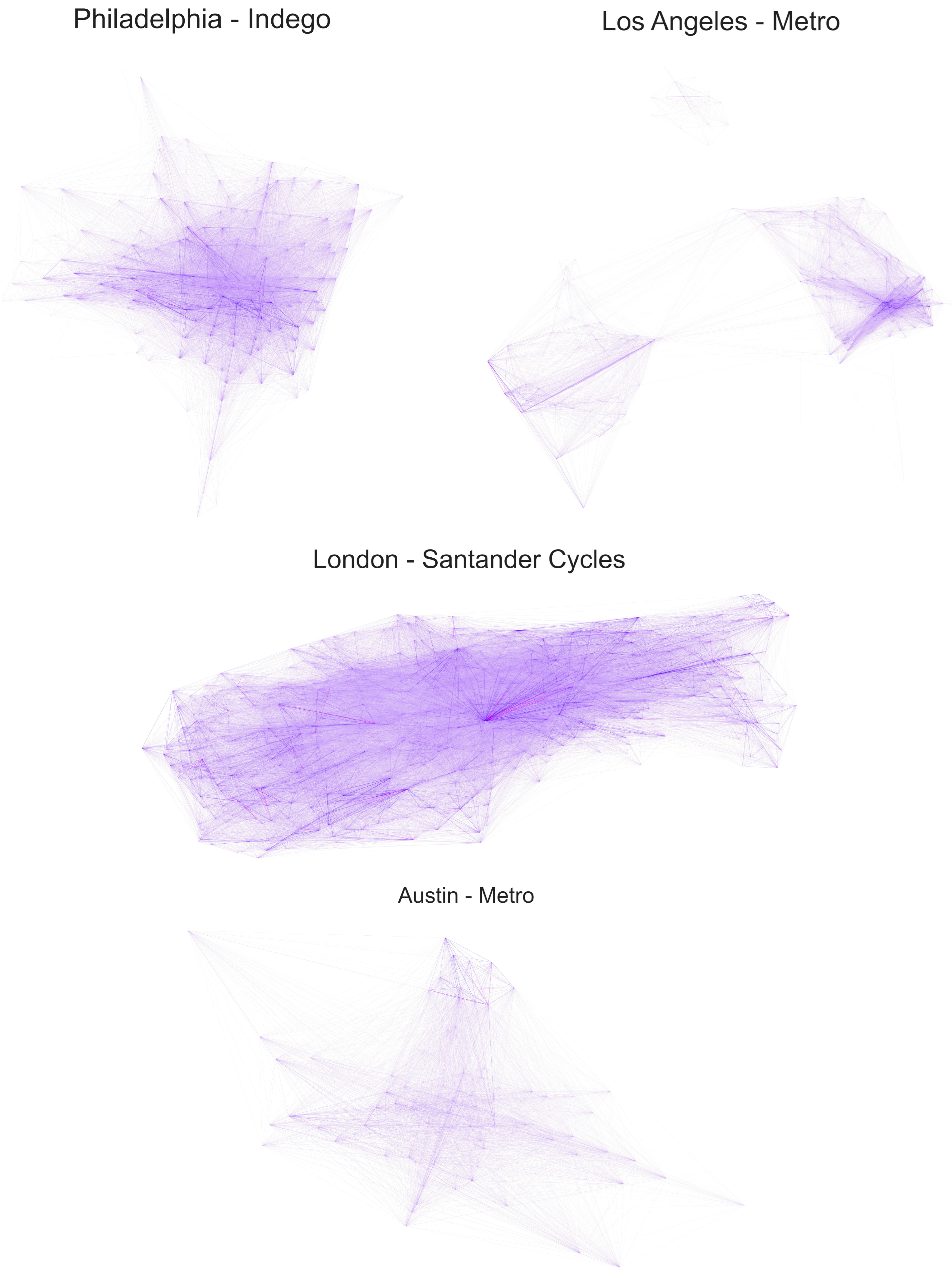
The graphic illustrations below (
Figure 1) give a visual interpretation of the spread and frequency of trips made by shared bicycles around the studied cities. These diagrams explicitly highlight the concentration and level of trips heading to and from the city centres. Note: Metro has bike sharing stations in various separate neighbourhoods across Los Angeles.
4.2. Random Forest (RF)
A RF was used to predict whether a customer chose an ebike when both conventional and electric bicycles were available to the customer. As said before, the evaluation criteria of the model are high accuracy and minimising the share of false negatives. A false negative prediction is, in this study, a customer who used a bicycle in reality when the machine learning algorithm predicted that the customer would use an ebike. This situation should be avoided as it would be a waste of business resources to provide an ebike if it is not required. In the same way, it would be unfair to accuse a bike sharing operator of not providing enough ebikes, despite it only being a false negative prediction by the machine learning algorithm. In short, the machine learning algorithm should only predict an ebike if it is certain that one is requested. The accuracy is shown in
Table 2. The RF for Santander Cycles in London has the best prediction accuracy of 85% followed by Metro in Los Angeles and Austin with 75% and 73% accuracy, respectively. These are within the range of accuracies of RFs used to predict mode choice published in the literature: 62.3% [
18], 70.1% [
15], 81.7% [
14], 85% [
16], 85.6% [
21], and 91.4% [
19]. Zhou et al. [
14] reported a recall value of 79.6% for their RF used to predict whether people prefer a taxi or bike sharing, which is similar to the recall values of the RF classifiers in this study. The RFs were also calculated assuming a 15 min maximum parking duration for ebikes. The results are more or less the same.
Of those trips where no ebikes were available in the Santander Cycles system, 26% of customers are predicted to choose an ebike instead of a conventional bicycle. For Indego and Metro in Los Angeles and Austin, around 59% to 80% are predicted to have chosen an ebike if it were possible.
4.3. Deep Neural Network (DNN)
Table 3 shows the results for the DNN. The best DNN in terms of accuracy and recall is Santander Cycles in London (i.e., ≥84%). The performance for these DNNs are within a similar range of accuracies of neural networks used to predict mode choice in the published literature: 60.6% [
19], 64.6% [
21], 61.2% to 70.6%. [
20], and 84.37% [
17]. The share of false negatives is rather low for all systems apart from Indego in Philadelphia.
The SMOTE-NC generally increases the accuracy slightly compared to adjusting the class weights. However, the recall is, in most but not all cases, better when adjusting class weights.
Figure 2 depicts the predicted share of ebikes for trips where no ebike was available. Santander in London, which has the highest prediction accuracy, has the lowest predicted ebike share of around 21% to 27%. The share for all the other systems is much higher. As the prediction accuracy is not perfect for these, the results should be regarded with caution.
4.4. Removing False Negatives Using the DNN
False negatives mean that a customer who does not want to use an ebike is predicted as wanting one by the DNN. This would lead to an overestimation of the demand for ebikes. The threshold when the output of the DNN is considered to be an ebike is reduced so that only 1% or 0.5% of the output is a false negative. As shown in
Figure 3 and
Figure 4, even if the share of false negatives is only 1% or 0.5%, the proportion of trips where an ebike would have been hired, if available, for Santander Cycles is still 20% to 27%. The share of false negatives is less than 0.5% even within the normal threshold for Santander Cycles when the imbalance is addressed using class weights.
For most bike sharing system, between 18% and 32% of the customers are predicted to use an ebike if one is available, allowing for only a 1% share of false negative predictions. This reduces to 12% to 23% when the share of false negatives is reduced to 0.5%. The only exception is Metro in Austin, were the share for ebikes is predicted to be between 61% and 84%.
4.5. Feature Importance
The feature importance of the random forest for Santander Cycles in London (maximum parking duration 2 h) was calculated using two different methods. The temperature is the most important feature for the impurity-based calculation with a mean decrease in impurity of 0.262. This is followed by distance, average wind speed, and the difference in altitude between the start and end stations. The mean decrease in impurity ranges from 0.116 to 0.169. The number of intersections (0.092) and precipitation (0.072) are of average importance. The time of the day, day of the week, and season have the smallest influence.
The results of the permutation feature importance are relatively similar, with the travel distance, temperature, wind speed, intersections, altitude difference, and time of the day being the most important features.
5. Discussion and Conclusions
This study uses historical trip data to predict the demand for ebikes when none are available. Using only those trips where the customer has the choice between both ebikes and normal bicycles, DNNs and RFs are trained to gain an understanding of the current demand for ebikes. These DNNs or RFs are then used to predict the demand for ebikes from customers that rent a bicycle at a time when no serviceable ebike is available to them. The accuracy of the RF classifier is similar or slightly better than the accuracy of the DNN. In terms of recall, both performances are comparable.
Even if the share of false negatives is reduced to 1%, it is predicted that, for most bike sharing systems, between 18% and 32% of the customers would use an ebike if one is available, depending on the bike sharing system. This shows that, for all four bike sharing systems, there are still customers who would like to use an ebike but cannot do so due to their lack of availability.
The results are as expected given that bike sharing operators are most likely optimising the availability of ebikes to maximise their usage. Therefore, the share of trips where no ebike is available to a customer who wants one is expected to be low.
For the Santander Cycle in London dataset, the temperature, distance, average wind speed, and altitude difference between the start and end stations are the most important features, whilst the day of the week and season have only limited influence.
The proposed method will hopefully inspire bike sharing operators to use data-driven methods to predict the unmatched demand for ebikes in their own systems. In the same way, competitors could apply this method to predict when and where the demand for ebikes cannot be met by the another provider and specifically place their ebikes in these locations—possibly even at a higher price.
Policymakers can also use this method to see whether the bike sharing operator is too focussed on profits and ignores the many unhappy customers who cannot ride an ebike, as providing one would be unprofitable; or the opposite: whether the operator is more focussed on keeping the customers happy even though providing some of the ebikes might be unprofitable. Especially due to the ever pressing need to encourage a mode change towards sustainable modes of transport, the customer satisfaction of ebike sharing is key.
Future work should investigate whether adding additional features improves the accuracy of the prediction. These features could be, for example, the age of the customer and their previous choices, etc. Further research should also investigate whether increasing the number of ebikes further is financially viable. Just because one customer likes to use one, does not make it a good business strategy. Ways to validate the prediction of the machine learning algorithms should be investigated by asking customers whether they would have wanted an ebike when none were available.


