Two-Stage Optimization Scheduling of Virtual Power Plants Considering a User-Virtual Power Plant-Equipment Alliance Game

Abstract

Distributed renewable energy, loads, and power sources can be aggregated into virtual power plants (VPPs) to participate in energy market transactions and generate additional revenue. In order to better coordinate the transaction relationships among various entities within VPPs, this paper proposes a two-stage optimization model for VPPs that considers the user-VPP-equipment alliance. Firstly, starting from the basic structure of VPP, it is proposed to divide the alliances in VPP into two alliances: demand-side user-VPP and supply-side equipment-VPP. And a VPP optimization framework considering the cooperative game of the user-VPP-equipment alliance has been established. Then, a two-stage optimization model for VPPs was established considering the cooperative game of user-VPP-equipment alliance. The day-ahead optimization model takes economic and social benefits as the dual objectives, and the intraday optimization model aims to minimize the cost of deviation penalties. Secondly, taking into account the risk levels and comprehensive marginal benefits of various entities within the VPP, a profit distribution method combining improved Shapley values and independent risk contribution theory is adopted to allocate the total revenue of the VPP. The case results show that the operating cost has been reduced by 5.75%, the environmental cost has been reduced by 4.46%, and the total profit has increased by 29.52%. The model can improve the overall efficiency of VPPs.

1. Introduction

Traditional fossil energy consumption has caused serious pollution in the environment. In order to achieve sustainable development in the economy, environment, and other aspects, it is necessary to adjust the energy structure, vigorously develop clean energy, and reduce the use of fossil fuels [1]. However, both wind and solar energy are limited by natural conditions such as weather, resulting in their randomness and intermittency [2]. In addition, the cost of connecting distributed power sources to the power grid is also relatively high [3]. At present, countries have provided generous subsidies to encourage renewable energy generation, leading to explosive growth of distributed intermittent power generation equipment and affecting the stability of the power grid supply [4]. In order to coordinate the contradiction between the power system and distributed power sources and address the many challenges brought by new energy generation to the power system, scholars have proposed the concept of virtual power plants (VPPs). VPPs are one of the important forms of the future energy internet [5]. VPPs utilize advanced information and communication technology to achieve aggregation and coordinated optimization of distributed energy, energy storage systems, controllable loads, electric vehicles, etc. [6] and will actively participate in the power exchange with the main grid electricity market, resulting in profit streams that also bring certain benefits to power plants [7]. From the perspective of individual rationality, the prerequisite for each entity to participate in a VPP operation is to be able to obtain excess profits [8]. Strengthening the collaborative scheduling of various participating entities within VPPs is the main way to achieve excess profits. In addition, the reasonable distribution of excess profits is also a favorable way to stimulate the initiative of various participating entities. Therefore, how to achieve VPP optimization scheduling and reasonable profit distribution is the key to its effective operation.

Domestic and foreign scholars have conducted in-depth research on the participation of distributed energy sources such as distributed power sources, energy storage systems, and controllable loads in the operation of power grids and have made practical progress. Some scholars have begun to study the optimal scheduling problem of VPPs. Li, Q. et al. [9] propose a two-stage scheduling framework for VPPs to address the uncertainty of wind power plants, photovoltaics, loads, and prices in the power system. The framework includes a day-ahead scheduling stage and day adjustment stage. Liu, J. et al. [10] proposes a two-stage optimization model for VPPs consisting of interconnected micro-grids with different load curves to provide demand-side frequency control auxiliary services. Gulotta, F. et al. [11] proposed a novel rolling horizon-based VPP energy resource uncertainty short-term scheduling model based on stochastic programming. Zhang, T. et al. [12] proposed a two-part price leasing mechanism for shared energy storage that considers market prices and battery degradation based on the flexibility of the energy storage sharing model. Yang, C. et al. [13] proposed a day-ahead optimal bidding strategy model for VPPs that includes energy, reserve, and regulatory markets. This model considers economic penalties beyond reserve capacity and optimizes the allocation of reserve capacity to maximize overall profits. This article studies the optimal scheduling problem of VPPs. In order to maximize the operational profit of VPPs, taking into account the uncertainty of comprehensive demand response, renewable energy output, and load forecasting, NSGA-II is used to solve the model to alleviate the slow convergence and severe local optimization problems caused by excessive decision variables and constraints in the energy system comprehensive scheduling optimization process and effectively solve the problem of absorbing new energy power through these controllable energy sources.

A VPP participates in market operations as a whole and coordinates internal resources. It can sell surplus electricity to the electricity market or purchase electricity from the market to meet load demand and achieve optimal economic efficiency [14]. At present, research on VPP optimization scheduling focuses on maximizing the economic benefits or minimizing the costs of VPPs as the objective function, and there is little literature related to environmental benefits. Wang, Y. et al. [15] studied the interaction mechanism between green certificates and carbon trading and market environmental constraints and proposed a bidding strategy model for maximizing the economic benefits of VPPs. Mei, S. et al. [16] proposed a multi-market model for multi-objective optimization from the perspectives of comfort and economy, which is used to develop the optimal bidding strategy for VPPs. Nokandi, E. et al. [17] proposed a two-stage model for VPP joint energy and reserve scheduling considering local intraday demand response (DR) exchange markets. The upper layer is a VPP with the goal of maximizing its profits, while the lower layer is an internal load aggregator with the goal of maximizing its social welfare. Cao, J. et al. [18], considering the uncertainty of renewable energy and load, proposed a two-stage economic dispatch strategy for VPPs with multi-time scale optimization, including long-term day-ahead dispatch and short-term real-time dispatch. Liu, H. et al. [19] proposed a two-level coordinated scheduling strategy based on Stackelberg game theory to minimize scheduling costs and maximize the income of electric vehicle owners.

In practical applications, in order to improve the revenue of VPPs, it is necessary to minimize the energy storage on the user side as much as possible. After determining the benefits of VPPs, how to achieve reasonable benefits for distributed entities such as distributed generation, energy storage system, and controllable loads is the key to achieving power collaborative management. Zhang, T. et al. [12] proposed an auxiliary VPP profit distribution method based on an improved Shapley value method and minimum deviation algorithm to reflect the true contributions of participants and balance their interests. Fang, F. et al. [20] developed a new profit distribution method for multiple distributed energy sources coexisting in cogeneration VPPs. Wang, X. et al. [21] proposed a profit distribution mechanism that considers the true contribution of each participant to address the problem of multiple participants coexisting in a wind storage joint system. Rahmani-Dabbagh, S. et al. [22] proposed a comprehensive profit distribution framework based on integrated distributed energy virtual internal transactions. Cremers, S. et al. [23] designed a new method for precise Shapley value calculation by clustering consumers into a smaller number of requirement configuration files. Wang, Y. et al. [24] proposed an improved profit distribution method that combines the Shapley value and nucleolus methods.

In summary, there are still shortcomings in existing research on VPP optimization scheduling and benefit allocation. In order to better coordinate the transaction relationships among various entities within VPPs, this paper proposes a two-stage optimization model for VPPs that considers the user-VPP-equipment alliance. Compared with existing similar works, the main innovations of this article are as follows:

(1) A user-VPP-equipment cooperation alliance structure has been proposed. The article establishes the basic structure of a VPP and analyzes the interaction logic between its internal elements. From the perspective of energy supply and consumption, the cooperative alliance in VPPs was innovatively divided into two alliances: demand-side user-VPP and supply-side equipment-VPP, and a user-VPP-equipment cooperative alliance was further established.

(2) We have established an optimization framework for VPP that considers the cooperative game of user-VPP-equipment alliance. Based on the analysis of the two alliances of user-VPP and equipment-VPP, this framework clarifies the game relationships of all parties in VPPs, and further demonstrates the optimization framework of the VPP game model.

(3) A two-stage optimization model for VPPs considering the user-VPP-equipment alliance cooperative game was established. This model includes two time stages: day-ahead and intraday. Among them, the day-ahead optimization model takes economic and social benefits as dual objectives. The intraday optimization model aims to minimize the cost of deviation penalties.

(4) A new profit distribution mechanism has been proposed. Taking into account the risk levels and comprehensive marginal benefits of various entities within the VPP, a profit distribution method combining improved Shapley values and independent risk contribution theory is adopted to allocate the total revenue of the VPP.

The rest of this study is organized as follows: Section 2 provides a detailed description of a cooperative game-based VPP optimization framework. Section 3 provides a detailed explanation of the optimization model and constraints, as well as an introduction to the algorithm and implementation process. The effectiveness of the framework and model was verified through simulation results, and the simulation results were discussed and analyzed. The final part is the main conclusion drawn from this study.

2. VPP Bi-Level Optimization Theory Based on Cooperative Games

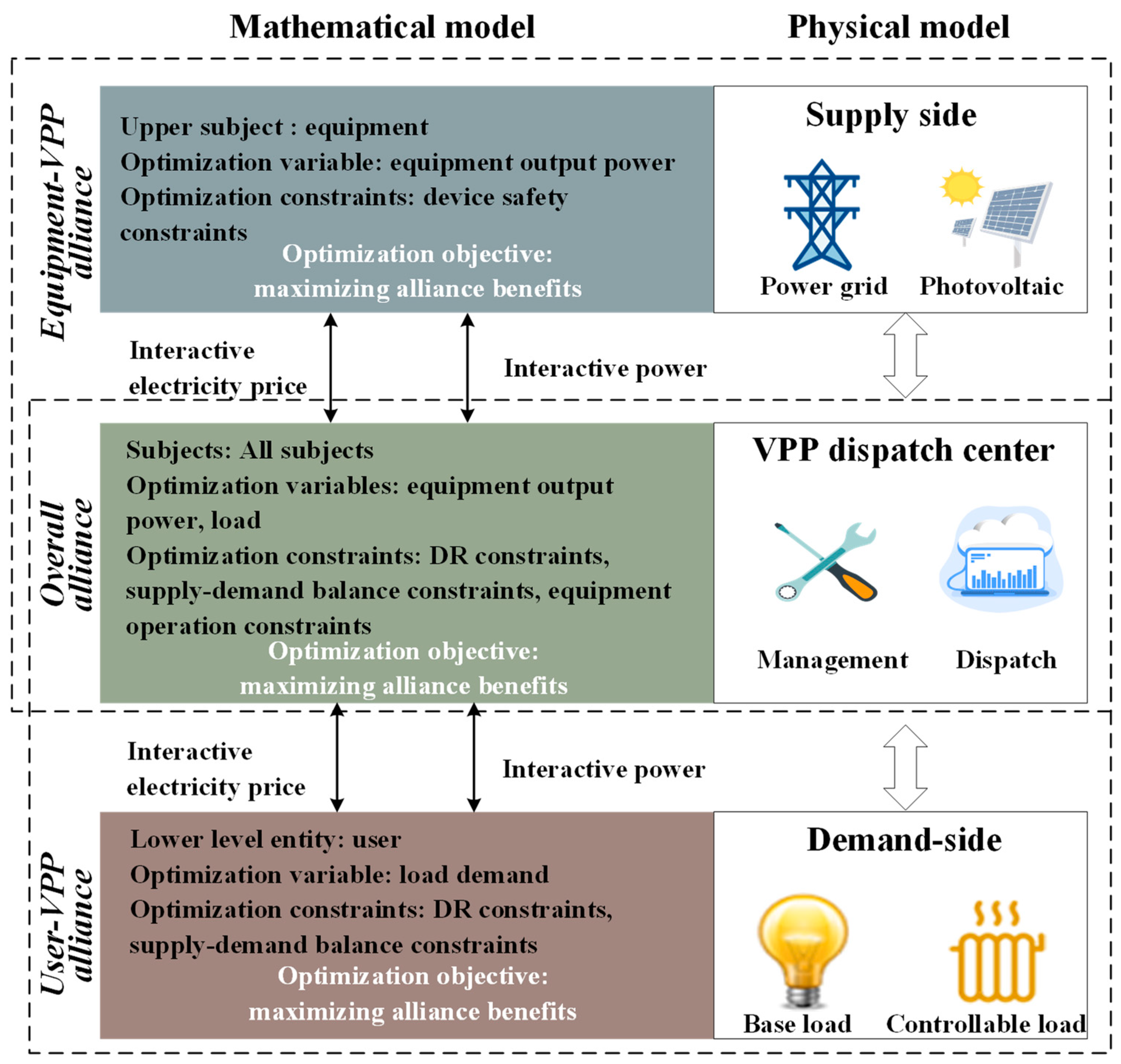
2.1. The Alliance Structure of VPP Cooperative Games

A VPP typically includes distributed power sources, energy storage devices, controllable loads, and other types and capacities of distributed energy [25], as shown in Figure 1. The aggregation of multiple distributed energy sources by a VPP can effectively improve the operational stability of regional power grids, promote the consumption of renewable energy, and obtain residual profits. That is, the coordinated operation profit of VPP is higher than the total profit of individual scheduling of distributed energy sources [26].

Under market conditions, the premise for various distributed resource operators to collaborate to form a VPP is based on the interests and demands of each entity, and these entities are assumed to be [i1, i2, …, i_n]. According to the idea of cooperative games, the interests of the subject can be divided into two parts: individual rationality and collective rationality [27,28].

(1) Individual rationality. For a cooperative game with distributable profits, the distribution vectors [v1, v2, …, v_n] are in line with individual rationality. The cooperative alliance will only be established if and only if each participant in the alliance S obtains a distribution utility that is not less than the utility obtained when they operate independently, namely [7]:

$$v(i)\ge u(i),\forall i\in A_{VPP}$$

(1)

where $v(i)$ is the distribution of entity i in the cooperative alliance, and $A_{VPP}$ is the cooperative alliance. $u(i)$ is the income of independent operation of entity i.

(2) Collective rationality. On the basis of satisfying individual rationality, its distribution vector [v1, v2, …, v_n] also needs to comply with collective rationality, if and only if the distribution utility obtained by the participants of alliance S is equal to the total alliance utility, that is:

$${\displaystyle \sum _{i=1}^{n}v(i)}=u(A_{VPP})$$

(2)

where $u\left(A_{VPP}\right)$ is the total revenue of alliance $A_{VPP}$.

Therefore, in order to meet the rational conditions of individuals and groups, the prerequisite for VPP cooperation is:

(1) To meet individual rational conditions, it is necessary to carry out operational optimization and demand response. The former can reduce operational costs and increase coordinated operational profits. The latter can derive cooperative value-added services through the large-scale operation of the VPP.

(2) To meet the conditions of collective rationality, it is necessary to fully distribute the profits of coordinated operation and ensure fair cooperation. Therefore, based on the research on the income cash flow of the VPP, a revenue allocation method based on the comprehensive contribution of partners is proposed to form a cooperative trading mechanism for the VPP, in order to reasonably allocate the operating income surplus.

Generally, a VPP can be divided into load sets with users as the main body and device sets with distributed power sources, energy storage devices, etc. as the main body. Therefore, in the existing electricity market, the bilateral fixed pricing mechanism of VPPs limits the flexibility and initiative of multiple parties to participate. However, when a strong alliance system is formed on both sides of supply and demand, all members aim for common benefits, which not only improves alliance benefits and individual benefits of members, but also strengthens the connection between supply and demand. Therefore, the forms of alliances in VPPs include the user-VPP alliance on the demand-side and the equipment-VPP alliance on the supply-side.

2.1.1. The User-VPP Alliance on the Demand-Side

(1)

Operation mode under non-cooperative game

Before establishing a cooperative game alliance between users and the VPP, it is first necessary to define separate operational models for both parties. Both user-side revenue and VPP revenue aim to maximize revenue [20].

$$\max F_{\mathrm{demand}}={\displaystyle \sum }_T^{t=1}{P}_{\mathrm{L},t}\Delta {\rho }_{\mathrm{s},t}\Delta t$$

(3)

$$\max F_{\mathrm{vpp}1}={\displaystyle \sum }_T^{t=1}{P}_{\mathrm{L},t}\left({\rho }_{\mathrm{s},t}-{\rho }_{\mathrm{b},t}\right)\Delta t$$

(4)

where $P_{\mathrm{L},t}$ is the traditional electricity demand on the user side at time t, kW; ${\rho }_{\mathrm{s},t}$, ${\rho }_{\mathrm{b},t}$ is the internal electricity selling price and purchasing price of VPP at time t.

In non-cooperative games, the closer to peak electricity consumption, the greater the interaction between the VPP and users in terms of electricity consumption. At this time, the VPP’s profits mainly come from the difference between internal electricity purchases and sale prices. The revenue of demand-side users is mainly determined by the changes in VPP electricity prices and their own electricity demand. There is no cooperative relationship between one VPP and another VPP, and the pricing process of a VPP does not consider the revenue of demand-side users.

(2)

Operation mode under a cooperative game

Users and the VPP form an alliance system with the goal of maximizing mutual benefits.

$$\max F_{\mathrm{vpp}-\mathrm{de}}=F_{\mathrm{vpp}1}+F_{\mathrm{demand}}$$

(5)

2.1.2. The Equipment-VPP Alliance on the Supply-Side

(1)

Operation mode under a non-cooperative game

$$\max F_{eq}=\sum _T^{t=1}\left[F_{\mathrm{gsell},t}-C_{\mathrm{G},t}\right]\Delta t$$

(6)

where $F_{\mathrm{gsell},t}$ is the electricity sales revenue, and $C_{\mathrm{G},t}$ is the cost of generating electricity for the unit.

$$\max F_{\mathrm{vpp}2}=\sum _T^{t=1}\left[F_{\mathrm{sell},t}-C_{\mathrm{buy},t}-C_{\mathrm{pv},t}-C_{\mathrm{bes},t}\right]\Delta t$$

(7)

where $F_{\mathrm{sell},t}$, $C_{\mathrm{buy},t}$, $C_{\mathrm{pv},t}$, and $C_{\mathrm{bes},t}$ are the VPP’s electricity sales revenue, the VPP’s electricity purchase cost, photovoltaic power generation cost, and energy storage system usage cost at time t.

(2)

Operation mode under a cooperative game [22,23]

Under cooperative games, the VPP and the equipment jointly form an alliance system, with the goal of maximizing the profits of the equipment-VPP alliance.

$$\max F_{\mathrm{vpp}-\mathrm{eq}}=F_{\mathrm{vpp}2}+F_{\mathrm{eq}}$$

(8)

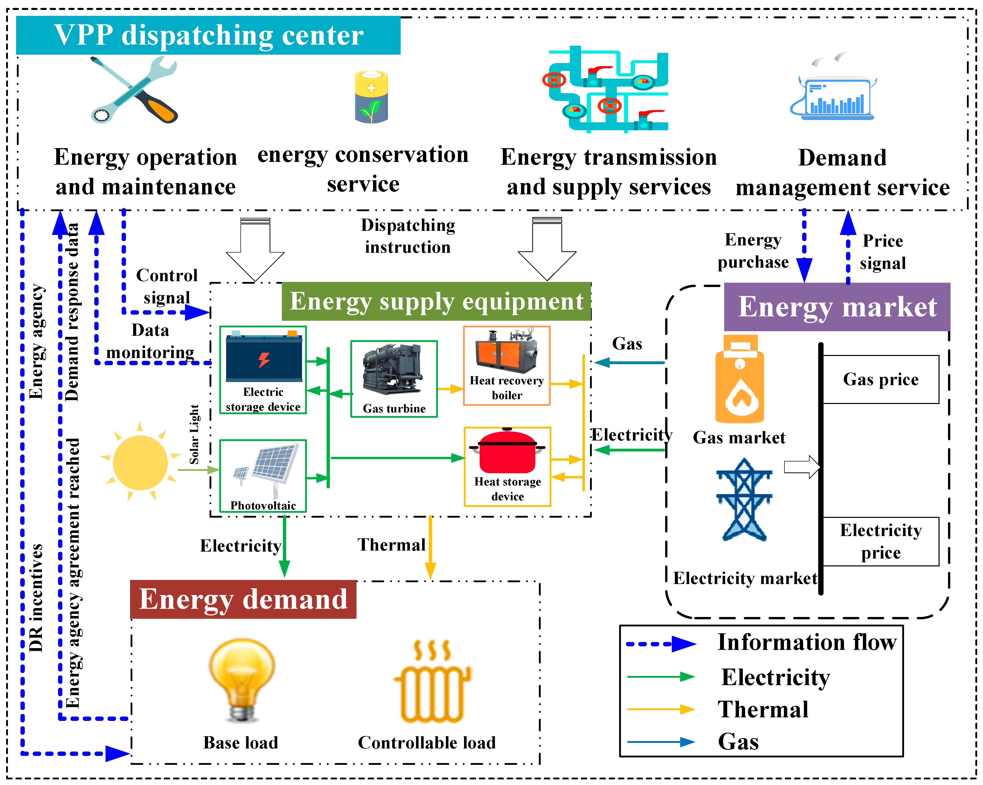
2.2. Optimization Framework for VPP Considering Cooperative Game of the User-VPP-Equipment Alliance

The optimization framework of VPP cooperative games considering the user-VPP-equipment alliance proposed in this article is divided into upper and lower layers from a supply and demand perspective, aiming to maximize the benefits of multiple parties through joint operation between different cooperative game alliances. The overall architecture is shown in Figure 2. The operation process of the entire two-layer cooperative game framework is as follows:

(1) The VPP formulates initial electricity purchase and sale prices as the initial equilibrium solution and notifies demand-side users of the electricity sale price. Demand-side users determine their own electricity demand based on the electricity price level;

(2) Lower-level users and the VPP form a user-VPP alliance and carry out cooperative games with the goal of maximizing common benefits until the game equilibrium is reached. They reasonably allocate the alliance’s benefits and obtain the electricity selling price and user electricity demand after the game;

(3) Based on the electricity demand and selling price of users obtained from the lower-level game, combined with the predicted output of renewable energy sources, the current internal load level of the VPP is determined;

(4) The VPP and the upper-level equipment form an equipment-VPP alliance and carry out cooperative games with the goal of maximizing common benefits until the game equilibrium is reached. And they conduct income distribution to obtain the electricity purchase price and interaction power with the equipment after the game;

(5) The VPP notifies the user side of the electricity purchase price set by the upper-level and replays the game at the lower level. The upper and lower levels continuously update their strategies based on this until they reach the equilibrium point of the double-layer model. The update and change of the electricity sale price at the lower level remain stable within a very small range as the equilibrium standard.

3. A Two-Stage Optimization Model for VPP Considering the User-VPP-Equipment Alliance

Based on the above analysis, not all decision variables need to be determined in advance during the VPP trading process. Some variables can be flexibly adjusted during the actual operation. Therefore, this article adopts a two-stage model to consider the impact of uncertainty in photovoltaic power generation output on bidding strategies. Figure 3 shows a two-stage optimization framework for VPP considering multi-agent cooperative games.

3.1. The First Stage: Day-Ahead Optimal Scheduling Model

3.1.1. Optimization Objective

Before the end of energy market transactions, the VPP system predicts the potential contribution of photovoltaic power generation, makes decisions with the goal of maximizing its own profits, and submits market bidding strategies in advance to develop unit output plans during the period. Therefore, based on cooperative games, this section mainly considers the cooperative alliance and social benefits of VPPs, and constructs the first-stage bidding model of the VPP.

(1)

Objective function 1: The best economic benefit of the VPP

The economic benefit of the VPP is characterized by the difference between the profit of VPP system operation and the cost of VPP system operation [1,3].

$$Max{F}_{VPP}^{EB}=R_{VPP}-C_{VPP}$$

(9)

where $F_{VPP}^{EB}$ is the social benefit of the VPP; $R_{VPP}$ is the benefits of VPP system operation; and $C_{VPP}$ the operation cost of the VPP system.

The benefits of VPP system operation mainly come from the remuneration obtained by participating in energy trading in the power market and the thermal market, as well as the economic compensation obtained by interrupting the load participating in power grid dispatching.

$$R_{VPP}=R_{VPP}^{dispatch-E}+R_{VPP}^{dispatch-T}+R_{I-Load}^{compensate}={\displaystyle \sum _{t=1}^T{p}_{s-E}{P}_{E-grid}(t)}+{\displaystyle \sum _{t=1}^T{p}_{s-T}}{P}_{T-grid}(t)+{\displaystyle \sum _{t=1}^T{C}_{I-Load}^t}{P}_{I-Load}(t)$$

(10)

where $P_{E-grid}(t)$ and $P_{T-grid}(t)$ are the exchange power between the ET-VPP system and the E-grid and T-grid, respectively; $P_{s-E}$ and $P_{s-T}$ are the electricity and thermal prices on the market; $C_{I-Load}^t$ is the benchmark economic compensation of interrupting load; and $P_{I-Load}(t)$ is the interruptible load capacity.

The operation cost of the VPP system mainly comes from the fuel cost (the cost of purchasing natural gas), the operation and maintenance cost of the unit, and the environmental emission cost of the system.

$$C_{VPP}=C_{fuel}+C_{operation}+C_{environmental}={\mathsf{\partial }}_{fuel}{\displaystyle \sum _{t=1}^T\frac{P_{CHP}^{}(t)+P_{GB}^{}(t)}{{\delta }_{GT}\times LH{V}_{NG}}}+{\displaystyle \sum _{t=1}^T{\displaystyle \sum _{i=1}^M{C}_i^{op}{P}_i^{}(t)}}+{\displaystyle \sum _{t=1}^T{P}_{en}^{}(t){\displaystyle \sum _{j=1}^N{\beta }_j^g(C_j^H+C_j^Y)}}$$

(11)

where $C_{fuel}$ is the operation cost of the NG supply module; ${\mathsf{\partial }}_{fuel}$ is the NG price; $LH{V}_{NG}$ is the low calorific value of natural gas; $P_{CHP\_n}(t)$ is the rated power of the CHP system; $P_{GB}^{}(t)$ is the rated power of the GB system; $C_i^{op}$ is the unit operation and maintenance cost of the energy supply unit in the system; $P_i^{}(t)$ is the rated power of the energy supply unit in the system, $P_{en}^{}(t)$ is the output power of the pollutant source in the system; ${\beta }_j^g$ is the amount of the pollutant $j$ produced by the unit output power of the pollutant source; $C_j^H$ is the basic discharge cost of per unit mass pollutant $j$; and $C_j^Y$ is the punishment cost per unit of mass pollutant $j$.

(2)

Objective function 2: The best social benefit of the VPP

In the process of construction, the VPP must not only maximize the economic benefits of the system but also take into account the social benefits related to human factors. VPP social benefits are characterized by DR electrical comfort. The higher the electrical comfort, the higher the VPP social benefits. The DR user’s electrical comfort is inversely related to the number of interruptible load (IL) calls and the total amount of transferable load (TL) translation [10,16].

$$Max{F}_{VPP}^{SB}=1-{\displaystyle \sum _{k=1}^V\left({\mathsf{\partial }}_1{\displaystyle \sum _{t=1}^T\raisebox{1ex}{${\Omega }_{1,k}^{}(t)$}\!\left/ \!\raisebox{-1ex}{${\pi }_{\max ,1,k}$}\right.+{\mathsf{\partial }}_2{\displaystyle \sum _{t=1}^T\raisebox{1ex}{${\Omega }_{2,k}^{}(t)$}\!\left/ \!\raisebox{-1ex}{${\pi }_{\max ,2,k}$}\right.}+{\mathsf{\partial }}_{3}0.5{\displaystyle \sum _{t=1}^T\raisebox{1ex}{$\left|P_{TL,k}^{}(t)\right|$}\!\left/ \!\raisebox{-1ex}{$P_{TL,k}^{\max }$}\right.}}\right)}$$

(12)

where $F_{VPP}^{SB}$ is the social benefit of the VPP. When IL and TL are not called at all during the scheduling period, the power comfort is the highest, $F_{VPP}^{SB}=1$; when the number of calls to IL reaches the upper limit and TL translates when the total amount reaches the upper limit, the electrical comfort is the lowest, $F_{VPP}^{SB}=0$; ${\mathsf{\partial }}_1$, ${\mathsf{\partial }}_2$ and ${\mathsf{\partial }}_3$ are the ratios of the total load of the class I IL, the class II IL, and the TL throughout the day to the total load of the VPP; ${\Omega }_{1,k}^{}(t)$, ${\Omega }_{2,k}^{}(t)$, $P_{TL,k}^{}(t)$ are the call state variables of the class I IL, the class II IL, and the TL; ${\pi }_{\max ,1,k}$, ${\pi }_{\max ,2,k}$ and $P_{TL,k}^{\max }$ are the maximum call numbers of the class I IL, the class II IL, and the TL in a single scheduling cycle.

3.1.2. Constraints

(1)

Energy Power Balance Constraints [11,24]

$$P_{E-load}(t)+P_{EES-char}(t)=P_{E-grid}(t)+P_{WT}(t)+P_{CHP}(t){\eta }_{CHP-E}+P_{EES-dis}(t)$$

(13)

$$P_{T-load}(t)+P_{TES\_char}(t)=P_{T-grid}(t)+P_{CHP}(t){\eta }_{CHP-T}+P_{GB}(t){\eta }_{GB}+P_{TES\_dis}(t)$$

(14)

where $P_{E-load}(t)$ and $P_{T-load}(t)$ are electrical load power and thermal load power, kW; $P_{EES-char}(t)$ and $P_{TES-char}(t)$ are the charging power of the EES and TES, kW; $P_{EES-dis}(t)$ and $P_{TES-dis}(t)$ are the discharging power of the EES and TES, kW; $P_{E-grid}(t)$ and $P_{T-grid}(t)$ are the exchange power between ET-VPP system and E-grid and T-grid respectively, kW; $P_{WT}(t)$ is the power of WT generators, kW; ${\eta }_{CHP-E}$ and ${\eta }_{CHP-T}$ are gas-to-electricity and gas-to-thermal efficiency of the CHP.

(2)

Energy storage operation constraint

The operation constraints of the energy storage system mainly include capacity constraints, charging state constraints and input, and output power constraints that TES and EES need to meet in the operation process [15].

• • Electric energy storage (EES)

$$SO{C}_{\min }\le SOC(t)\le SO{C}_{\max }$$

(15)

$$\{\begin{array}{c}0\le P_{char}(t)\le P_{char\_\max }{\varpi }_{BA\_s}\\ 0\le P_{dis}(t)\le P_{dis\_\max }{\varpi }_{BA\_r}\\ {\varpi }_{BA\_s}+{\varpi }_{BA\_r}\le 1\end{array}$$

(16)

$$\{\begin{array}{c}{P}_{char\_\max }=\min \left\{I_{char}^{\max }{V}_{bat},\frac{\left[SO{C}_{\max }-SOC(t)\right]Q_{\max }}{{\gamma }_{char}\Delta t},P_{inv}\right\}\\ P_{dis\_\max }=\min \left\{I_{dis}^{\max }{V}_{bat},\frac{\left[SO{C}_{\max }-SOC(t)\right]Q_{\max }{\gamma }_{dis}}{\Delta t},P_{inv}\right\}\end{array}$$

(17)

$$SO{C}_{start}(t)=SO{C}_{end}(t)$$

(18)

where $SO{C}_{\min }$, $SO{C}_{\max }$ are the upper and lower limits of the remaining capacity, respectively; ${\varpi }_{BA\_s}$, ${\varpi }_{BA\_r}$ is the efficiency of battery charging and discharging, respectively; $I_{char}^{\max }$, $I_{dis}^{\max }$ are the maximum charge and discharge current allowed by the battery; and $SO{C}_{start}(t)$, $SO{C}_{end}(t)$ are the remaining capacity of the start time and the end time in a scheduling period.

• b.

  Thermal energy storage (TES)

$$Q_{T\_\min }\le Q_T(t)\le Q_{T\_\max }$$

(19)

$$\{\begin{array}{l}0\le P_{TES-dis}(t)\le P_{TES-dis-\max }{\varpi }_{T\_st}\\ 0\le P_{TES-char}(t)\le P_{TES-char-\max }{\varpi }_{T\_re}\\ {\varpi }_{T\_st}+{\varpi }_{T\_re}\le 1\\ Q_T\left(t\right)=Q_T\left(t-1\right)+{\varpi }_{T\_re}{P}_{TES-char}(t)-P_{TES-dis}(t)/{\varpi }_{T\_st}\\ P_{TES-dis}(t)P_{TES-char}(t)=0\end{array}$$

(20)

$$Q_{T\_start}=Q_{T\_end}$$

(21)

where, $Q_{T\_\min },Q_{T\_\max }$ are the upper and lower limits of the remaining TES capacity, respectively; $P_{TES-dis-\max }$ and $P_{TES-char-\max }$ are the maximum limits for TES energy storage and release, respectively; ${\varpi }_{T\_st}$ and ${\varpi }_{T\_re}$ are the efficiency of TES storage and release, respectively; and $Q_{T\_start}$ and $Q_{T\_end}$ represent the remaining capacity of the start time and the end time in a scheduling period.

(3)

Operational constraints of the CHP [29,30]

$$0\le P_{CHP}(t)\le P_{CHP\_n}(t)$$

(22)

$$\Delta P_{CHP}^{\min }(t)\le P_{CHP}(t+1)-P_{CHP}(t)\le \Delta P_{CHP}^{\max }(t)$$

(23)

where $P_{CHP\_n}(t)$ is the rated power of the CHP system; and $\Delta P_{CHP}^{\max }(t)$ and $\Delta P_{CHP}^{\min }(t)$ are the upper and lower limits of the climbing rate of the CHP system, respectively.

(4)

Transmission constraints in the energy grid

$$\{\begin{array}{c}{P}_{E\_\min }\le \left|P_{E-grid}(t)\right|\le P_{E\_\max }\\ V_{i,\min }\le V_{i,t}\le V_{i,\max }\\ Q_{i,\min }^E\le Q_{i,t}^E\le Q_{i,\max }^E\\ \left|{\delta }_i-{\delta }_j\right|<{\left|{\delta }_i-{\delta }_j\right|}_{\max }\end{array}$$

(24)

$$P_{T\_\min }\le \left|P_{T-grid}(t)\right|\le P_{T\_\max }$$

(25)

where $P_{E\_\min }$ is the minimum power exchange between the E-grid and the ET-VPP system, kW; $P_{E\_\max }$ is the maximum power exchange between the E-grid and ET-VPP, kW; $V_{i,t}$ represents the voltage at node $i$; $P_i^E$ represents the active power at node $i$; $Q_i^E$ represents the reactive power at node $i$; $V_{\max }$, $V_{\min }$, respectively, represent the upper and lower limits of voltage at node i; $Q_{\min }^E$ and $Q_{\max }^E$, respectively, represent the minimum and maximum reactive power at node $i$; and ${\delta }_i$, ${\delta }_j$, respectively, represent the voltage phases at node $i$ and node $j$. $P_{T\_\min }$ is the minimum power of the natural T-grid to supply thermal to the system, kW; $P_{T\_\max }$ is the maximum power of the T-grid to supply thermal to the system, kW.

(5)

Load Response Constraints

DR constraints mainly refer to the power and time constraints that IL and TL must meet in response to VPP scheduling [18].

• • Interruptible Load operational constraints

The operation constraints of Class I interruptible load and Class II interruptible load are the same. The following interruptible load operation constraints are applicable to both types of interruptible load [16,17].

$${\Omega }_k^{}(t)\le {\pi }_{\max ,\mathrm{k}}$$

(26)

$${\displaystyle \sum _{l=t}^{t+T_{\max }}{\Omega }_k^{}(t)}\le T_{\max },t\in \left[1,T-T_{\max }\right]$$

(27)

$$\{\begin{array}{c}{\Omega }_k^s\le {\Omega }_k^{}(t)-{\Omega }_k^{}(t-1)+1\\ t\in 2\left[1,T-T_{\max }+1\right],s\in 2\left[t,T+T_{\min }-1\right]\end{array}$$

(28)

$${\Omega }_k^{}(t)=0,t\in {\Omega }_{IL,k}^{}$$

(29)

where ${\Omega }_k^{}(t)$ is the invocation state variable of IL; ${\pi }_{\max ,\mathrm{k}}$ is the upper limit of the invocation times of IL in a scheduling cycle; $T_{\max }$ and $T_{\min }$ are the maximum successive invocation times and the minimum successive non-invocation times of IL, respectively; and ${\Omega }_k^{}$ is the collection of non-callable periods.

• b.

  Transferable Load operational constraints

$${\displaystyle \sum _{t=1}^T{P}_{TL,k}^{}(t)}=0$$

(30)

$$-P_{TL,k}^{in}\le P_{TL,k}^{}(t)\le P_{TL,k}^{out}$$

(31)

$$0.5{\displaystyle \sum _{t=1}^T\left|P_{TL,k}^{}(t)\right|\le P_{TL,k}^{\max }}$$

(32)

$$P_{TL,k}^{}(t)=0,\forall t\in {\Omega }_{TL,k}^{}$$

(33)

where $P_{TL,k}^{out}$, $P_{TL,k}^{in}$ are the maximum of TL load migration and load migration; $P_{TL,k}^{\max }$ is the maximum of TL load migration; and ${\Omega }_{TL,k}^{}$ is the set of non-translational periods.

3.2. The Second Stage: Intraday Optimal Scheduling Model

3.2.1. Optimization Objective

After the uncertain parameters of photovoltaics are realized, based on the decision-making results of stage 1, the internal unit output is adjusted flexibly, so that the actual output of VPP meets the bidding output value of stage 1 as far as possible, and the real-time optimal dispatching strategy for the next day is obtained. Therefore, in the objective function of stage 2, the punishment cost due to the deviation of actual output and the punishment cost of wind abandonment need to be strictly considered, so as to improve the level of clean energy absorption [14,25].

$$Min{F}_{VPP}^{Fine}=C_{fine}^{BP}+C_{fine}^{AW}$$

(34)

$$C_{fine}^{DR}=\{\begin{array}{cc}{\lambda }_t^{BP,fin{e}^{+}}\Delta Q_{}^{BP}(t)& if,\Delta Q_{}^{BP}(t)\ge 0\\ \left\{\begin{array}{cc}{\lambda }_t^{BP,fin{e}^{1-}}\Delta Q_t^{BP}& ,\left|\Delta Q_{}^{BP}(t)\right|\le 0.5Q_{VPP}^{BP}\\ {\lambda }_t^{BP,fin{e}^{1-}}0.5Q_{VPP}^{BP}+{\lambda }_t^{BP,fin{e}^{2-}}(\Delta Q_{}^{BP}(t)-0.5Q_{VPP}^{BP})& ,0.5Q_{VPP}^{BP}\le \left|\Delta Q_{}^{BP}(t)\right|\le Q_{VPP}^{BP}\end{array}\right\}& if,\Delta Q_{}^{BP}(t)\le 0\end{array}$$

(35)

$$C_{fine}^{AW}={\lambda }_t^{AW,fine}{Q}_t^{AW}$$

(36)

where $F_{VPP}^{Fine}$ is the punishment cost of VPP participating in market scheduling; $C_{fine}^{AW}$ is the punishment cost of wind abandonment; $C_{fine}^{BP}$ is due to the deviation of actual output; ${\lambda }_t^{AW,fine}$ is the punishment coefficient of wind abandonment; $Q_t^{AW}$ is the abandoned wind volume; $\Delta Q_{}^{BP}(t)$ is the output deviation; ${\lambda }_t^{BP,fin{e}^{+}}$ is the punishment coefficient of output deviation ($\Delta Q_{}^{BP}(t)\ge 0$); ${\lambda }_t^{BP,fin{e}^{1-}}$ and ${\lambda }_t^{BP,fin{e}^{2-}}$ are the punishment coefficient of output deviation ($\Delta Q_{}^{BP}(t)\le 0$); and $Q_{VPP}^{BP}$ is the bidding power optimized in the first stage.

3.2.2. Constraints of the Second Stage

The other constraints of the second stage optimization are the same as those of the first stage optimization, as shown in Formulas (13)–(36).

3.3. Benefit Allocation Method Considering Risk and Contribution

The uncertainty risk of demand-side resources often affects the total revenue of virtual power plants, so the magnitude of risk should also be considered as one of the bases for profit distribution. And the profit distribution plan of the demand-side resource alliance must also meet the core theory of cooperative games [31]. Therefore, this article adopts an allocation method that combines the improved Shapley value method and the independent risk contribution theory.

3.3.1. Using the Theory of Risk Contribution to Determine the Magnitude of Risk

The independent risk contribution theory, incremental risk contribution theory, and marginal risk contribution theory are widely adopted in the risk contribution theory. In this article, it is assumed that the uncertainties between demand-side resources are independent of each other. Therefore, the independent risk contribution theory is used to decompose the contribution of demand-side resources to the total risk of virtual power plants. The specific expression is:

$$C_{i,\mathrm{SAC}}=\rho \left(L_i\right)$$

(37)

where $C_{i,\mathrm{SAC}}$ is the independent risk contribution of participant i; $L_i$ represents the risks brought by participant i participation in the alliance; and $\rho (·)$ is the risk evaluation function. $F_{c\mathrm{var}}$ is used to represent the risk evaluation function. The proportion factor ${\gamma }_i$ of risk size is:

$${\gamma }_i=C_{i,\mathrm{SAC}}/\sum _{j=1}^m{C}_{j,\mathrm{SAC}}$$

(38)

3.3.2. Using Improved Shapley Value to Determine Comprehensive Marginal Benefits

(1)

Shapley value

The Shapley value method is a game method used to solve income distribution or cost allocation problems in cooperative situations [23]. In the distribution process, income is allocated based on the marginal increase in revenue from the players in the alliance, allowing players who make more contributions to receive more distribution income. The idea of Shapley value is that the distribution income of players (VPP partners) is equal to the average marginal contribution of players to each alliance they participate in. The specific expression is [25]:

$${\phi }_i(V)={\displaystyle \sum _{i\in S}\frac{(S_i-1)!(n-S_i)!}{n!}}·(V(S)-V(S\backslash \{i\}))$$

(39)

where ${\phi }_i(V)$ is the distribution income of the i-th VPP collaborative combination; $S_i$ is the number of participants in alliance i; n is the total number of participants within the VPP; $V(S)$ is the overall operational coordination revenue of the VPP cooperation alliance; and $V(S\backslash \{i\})$ is the operational coordination income of the cooperative alliance after removing i from alliance S.

(2)

Improved Shapley value considering the comprehensive marginal contribution of the VPP

The Shapley value method only considers the economic marginal contribution of participants to the alliance, ignoring other contributions made by participants in the coordinated operation. In terms of the VPP, in addition to optimizing economic costs, the consumption of renewable energy and ensuring the reliability of grid operation are also important considerations. Based on the above ideas, the calculation method for income distribution $V(i)$ based on the comprehensive marginal contribution value is [26,27]:

$${\alpha }_i=V(n)\cdot \frac{{\phi }_i(V_c)}{{\displaystyle \sum _{i=1}^n{\phi }_i(V_c)}}$$

(40)

$${\phi }_i(V_c)={\displaystyle \sum _{i\in S}\frac{(S_i-1)!(n-S_i)!}{n!}}\cdot ({\displaystyle \sum _{j=1}^{m}V(S_{i,j})}-{\displaystyle \sum _{j=1}^{m}V(S_{{}_{i,j}}\backslash \{i\})})$$

(41)

where ${\alpha }_i$ is the actual income obtained by entity i based on the distribution of comprehensive benefit contributions; $V_c$ is the distribution value of comprehensive income; $V(S_c)$ is the comprehensive income obtained from the overall operation and coordination of the VPP cooperative alliance; $V(S_c\backslash \{i\})$ is the comprehensive income of the alliance S excluding i; and $V(S_{i,j})$ and $V(S_{{}_{i,j}}\backslash \{i\})$ are the equivalent economic values of the comprehensive benefits obtained by entity i in the cooperative alliance and the cooperative alliance after removing i, respectively. j is the j-th benefit indicator among comprehensive benefits.

3.3.3. Final Allocation Factor

$$a_i={\mathit{\sigma }}_i{\left[{\alpha }_i,{\gamma }_i\right]}^{\mathrm{T}}$$

(42)

where ${\mathit{\sigma }}_i$ is the weight of the specific gravity factor.

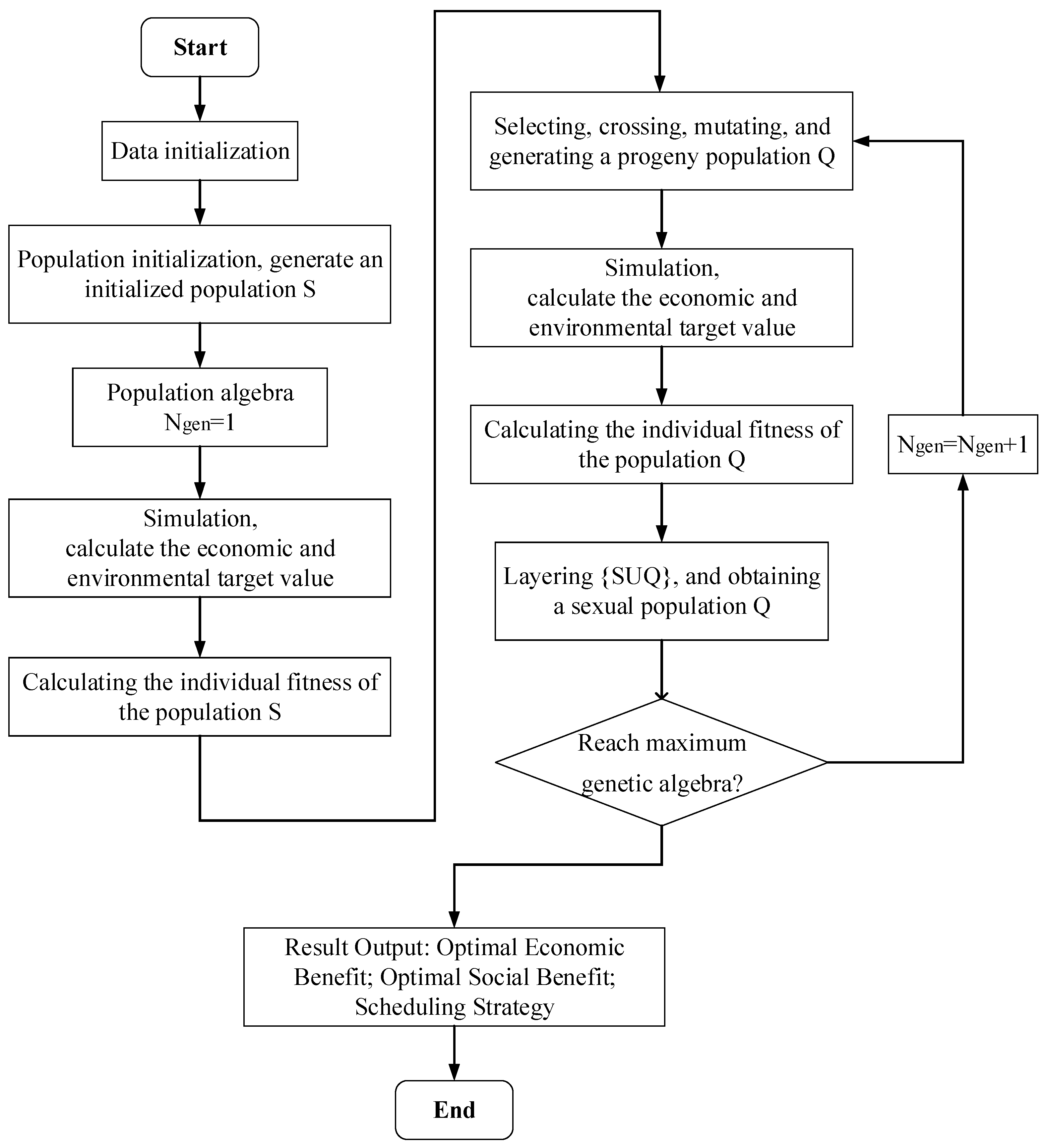
3.4. Model Solving Method

The first-stage day-ahead scheduling optimization model is a typical large-scale non-convex, non-linear, multi-objective optimization problem, which can be solved by NSGA-II algorithm. NSGA-II has strong variable processing ability, maintains the independence between optimization objectives, and better global optimization ability, and can effectively solve multi-objective problems. The NSGA-II algorithm can effectively solve this problem because of its strong variable processing ability, which maintains the independence between optimization objectives to the greatest extent and has better global optimization ability. The flow chart of the NSGA-II based on the day-ahead optimal scheduling model is shown in Figure 4.

After obtaining Pareto optimal frontier through NSGA-II, in order to obtain the practical control strategy quickly, the membership degree of each Pareto solution is calculated by introducing the preference factor to construct the comprehensive benefit index. The optimal scheme with the highest membership degree is the optimal compromise scheme.

$$f=Max\left[\phi \frac{F_{VPP}^{EB}}{F_{VPP}^{E{B}^{+}}}+(1-\phi )\frac{F_{VPP}^{SB}}{F_{VPP}^{S{B}^{+}}}\right]$$

(43)

where $\phi$ is a preference factor, and the range of the value is $0<\phi <1$, which is decided by the decision maker. The closer the value is to 1, it shows that the decision maker pays more attention to the economic benefits. On the contrary, if the decision makers pay more attention to the social benefits, $F_{VPP}^{E{B}^{+}}$ and $F_{VPP}^{S{B}^{+}}$ are the benchmark values, which are the maximum of the economic benefits and environmental benefits, respectively.

The second-stage bidding scheduling optimization model is a typical mixed integer linear programming problem, which can be modeled by YALMIP and solved by calling a solver. YALMIP is a toolbox in MATLAB, in which the model and algorithm are separated, and the appropriate solver can be selected automatically according to the type of solution required by the user. The user does not need to build the corresponding model for each algorithm.

The crossover rate of the NSGA-II algorithm is 0.9, the mutation rate is 0.2, the population size is 200, the maximum number of iterations is 150, the convergence gap value of CPLEX solver is set to 0.01%, and the maximum number of iterations of optimization is 30.

4. Data, Simulation Results, and Analysis

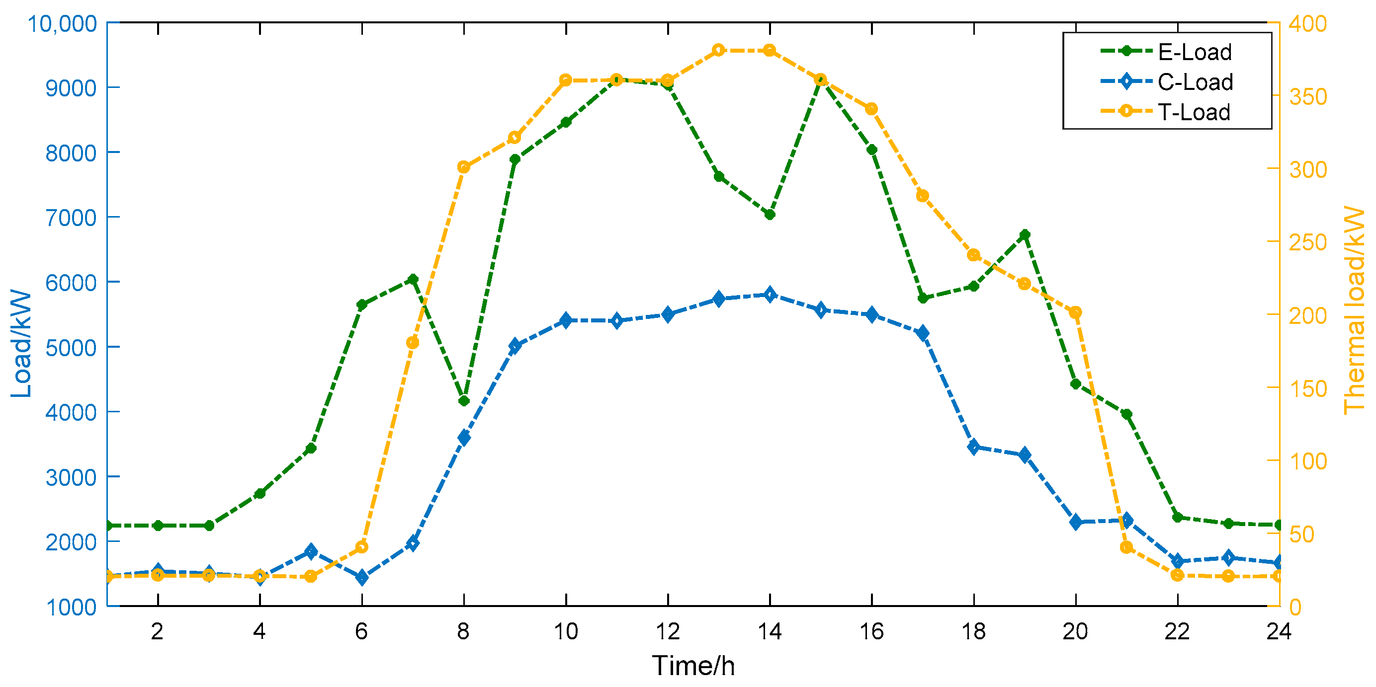
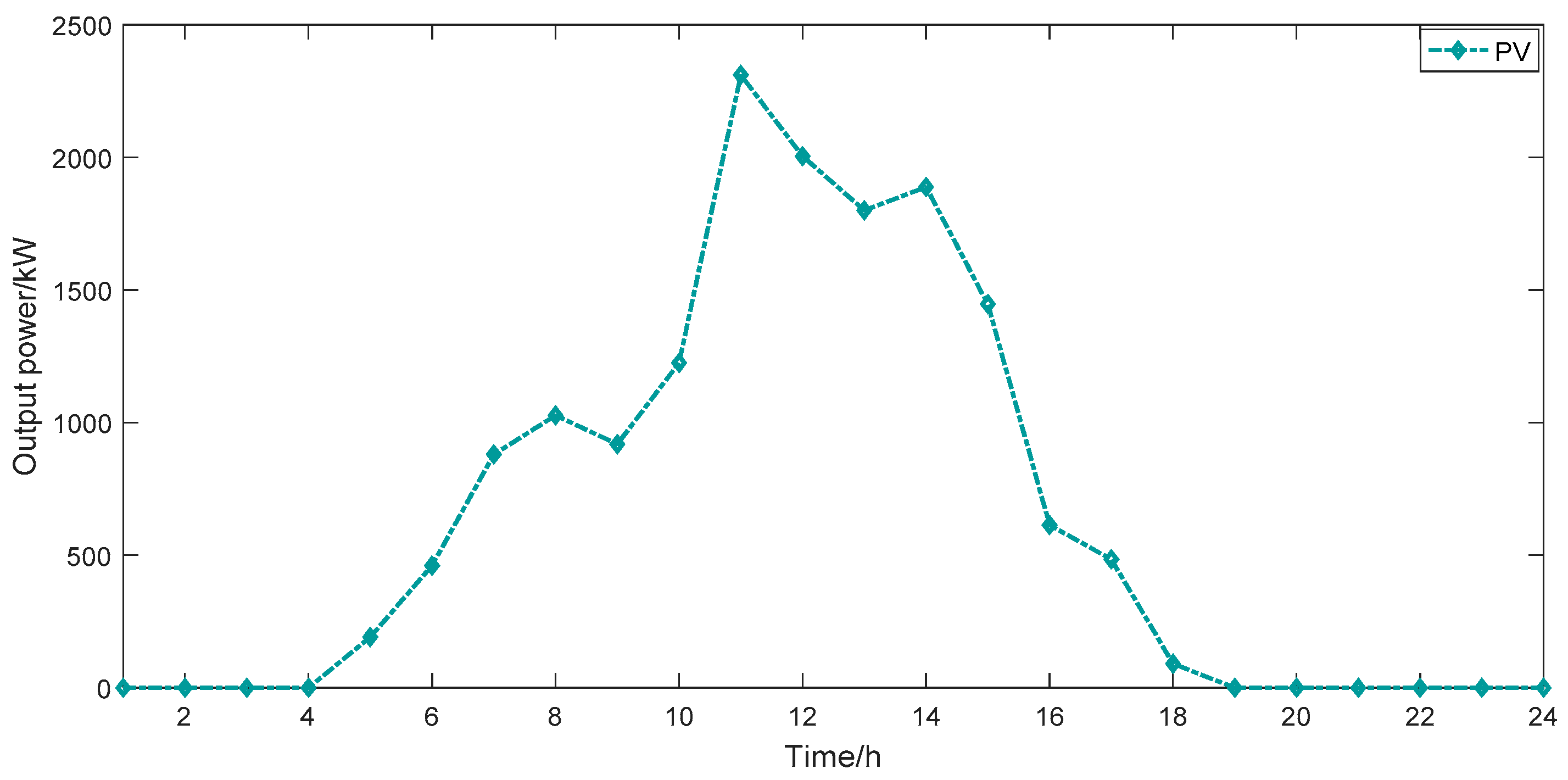
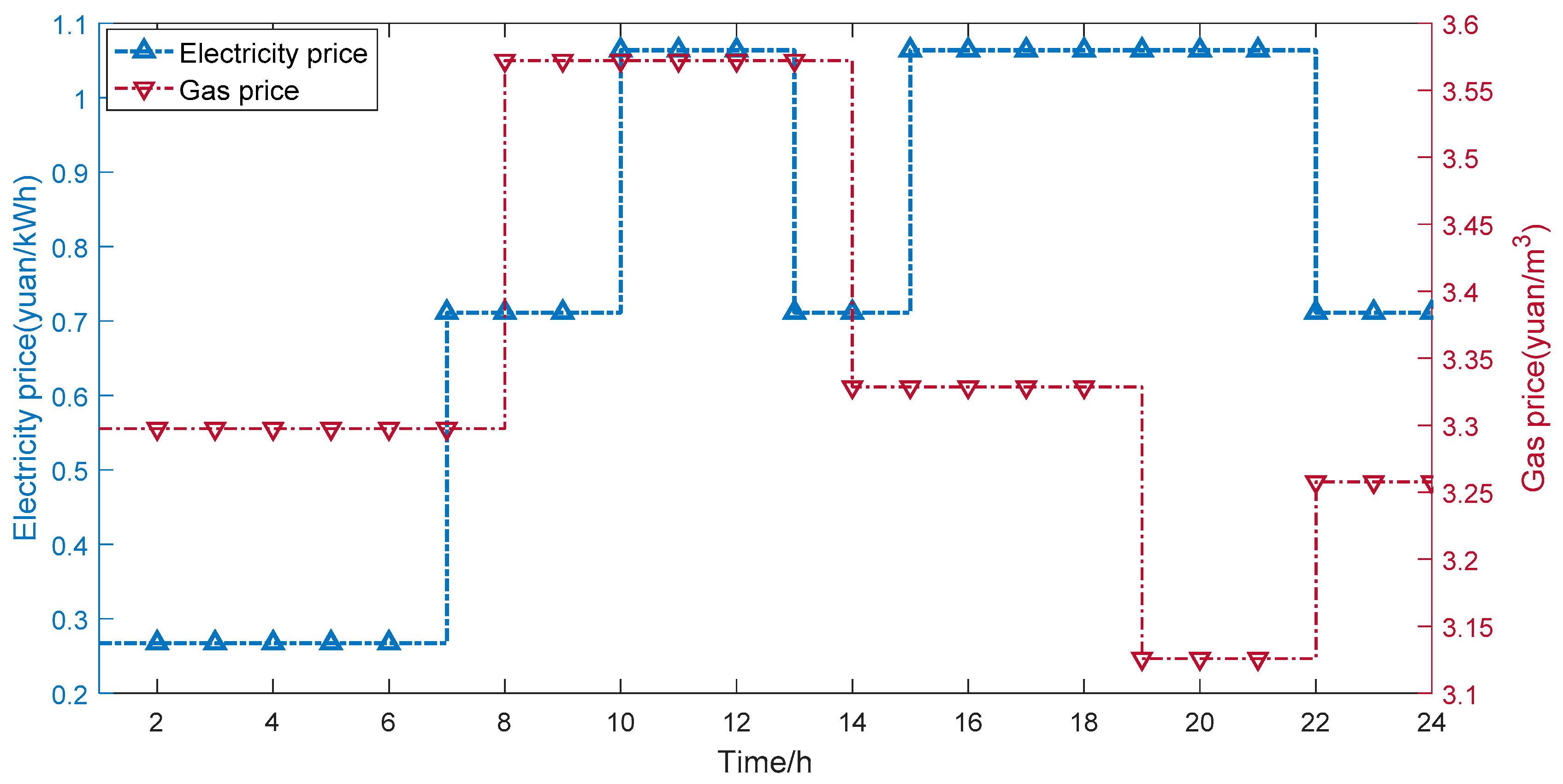
4.1. Data

This article takes a park in southern China as the research object for simulation analysis. The main load types of the park are electricity, heat, and cooling, including industries such as offices, catering, entertainment, and hotels. The energy system of the park includes equipment such as photovoltaic (PV) equipment, electric energy storage (EES) equipment, CCHP, and air conditioning (AC).

The operating cycle in the system is 24 h. The curves of renewable energy output, typical power load, heat load, and cooling load in the park are shown in Figure 5 and Figure 6. In addition, the existing energy supply equipment in the park mainly includes 4 sets of combined cooling, heating, and power supply units, 2.8 MW photovoltaic units, 4 MW air conditioning and refrigeration units, and energy storage systems. The capacity of the energy supply equipment is shown in

Table 1. Capacity of the energy supply equipment.

Symbol	Capacity	Operation Cost
PV	2.8 MW	0.65 yuan/kWh
EES	3 MWh	0.51 yuan/kWh
CCHP	8 MW	-

.

In addition, environmental cost is one of the factors that must be considered in the operation of VPPs, and it is also an important parameter for calculating the comprehensive contribution allocation value. While pursuing high economic benefits, it is necessary to ensure that pollutant emissions do not exceed standards; otherwise, high environmental costs will be incurred. The pollutant emissions and environmental cost factors are shown in

Table 2. Pollutant Emissions and Environmental Cost Factors [29,30].

Pollutants		SO2	NOx	CO2	CO
Emission	Coal (kg/t)	18	8	1731	0.26
	Gas (kg/106 m3)	11.6	0.0062	2.01	0
Environmental value (yuan/kg)		6.1308	26.00	0.0867	1.00
Punishment cost (yuan/kg)		1.00	2.00	0.01	0.16

.

The capacity of the energy supply equipment is shown in Table 2. The key operating parameters of each device are shown in

Table 3. Key operating parameters of each device.

Parameters	CCHP Electrical Efficiency	CCHP Thermal Efficiency	States of Charge of EES	States of Discharge of EES	EES Charge/Discharge Efficiency	Air Conditioning System Efficiency	Electrical ESS Dissipation Rate
Value	0.243	0.632	0.9	0.1	0.9	0.94	0.021

. The value of outsourced energy prices is shown in Figure 7.

4.2. Simulation Results

This section conducts simulation analysis based on the established two-stage operation optimization model and the improved Shapley value. By simulating the following three different energy supply modes, we study the impact of the VPP cooperative trading mode on equipment operation status and develop scheduling solution strategies for different modes.

Mode 1: The scheduling strategy of each energy supply unit is only formed by optimizing the scheduling in advance.

Mode 2: Based on the comprehensive marginal contribution, the cooperative relationship between various energy supply entities is considered, and the operational day-ahead strategy is formulated while meeting the maximization of the interests of the cooperating entities.

Mode 3: Based on the comprehensive marginal contribution, the cooperation relationship of each energy supply entity is considered, and the scheduling strategy of each energy supply unit is formed by the joint action of day-ahead scheduling and day-in scheduling.

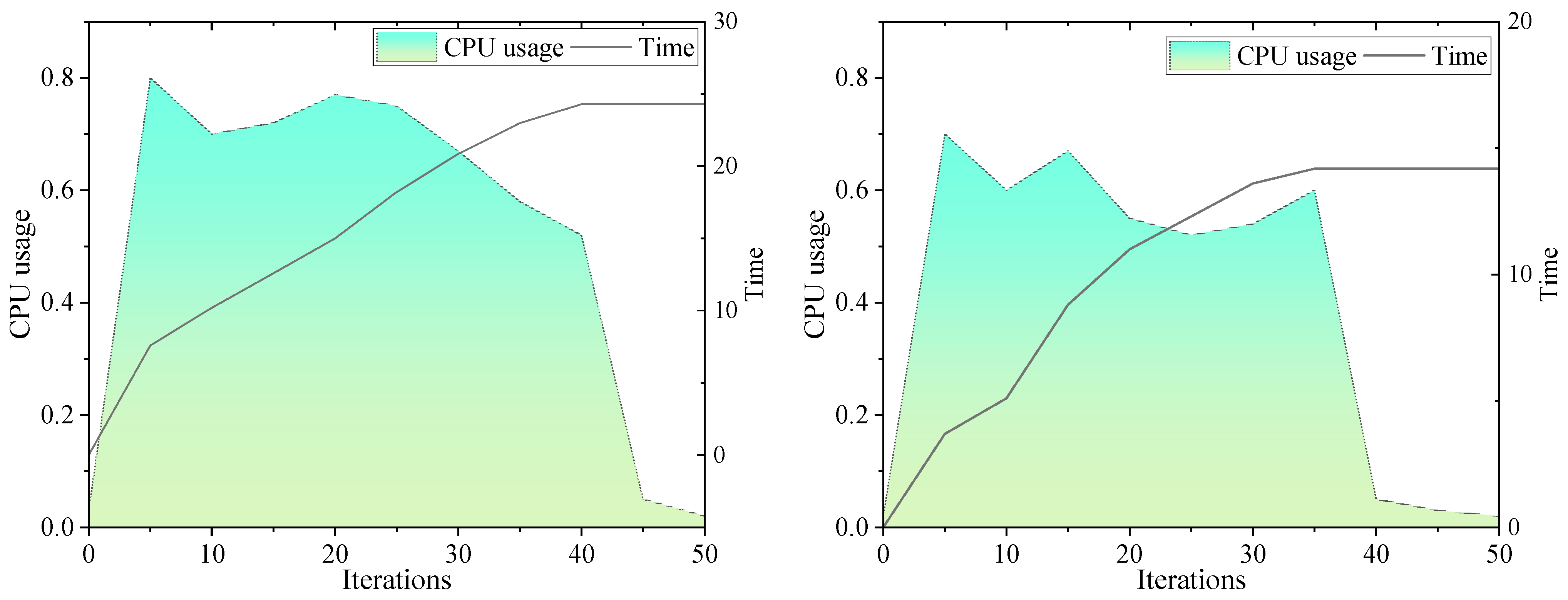
4.2.1. Operation Optimization Process

Based on the above three scenarios, this article applies the NSGA-II algorithm to the multi-objective optimization problem of the VPP. The initial population size is set to 1000 and the number of iterations is 100. The computer operating system version used is Windows 11, the CPU model is AMD Ryzen 7 4800 h with Radeon Graphics 2.90 GHz, and the RAM is 16 GB. The fitness curves for the first stage optimization and the second stage optimization of Mode 3 are shown in Figure 8, respectively. The CPU usage and runtime graph of NSGA-Ⅱ in different stages of Mode 3 are shown in Figure 9, respectively.

Obviously, when the algorithm runs in each stage of Mode 3, the fitness value continuously decreases. The first stage converges after 40 iterations, and the total running time of the program is approximately 24.2931 s. In the second stage, the optimal solution was found around the 35th generation, and the running time was approximately 14.1851 s. The CPU usage in the first stage is significantly higher than that in the second stage, due to the large computational workload in the first stage. Similar trends can be revealed in mode 1 and mode 2.

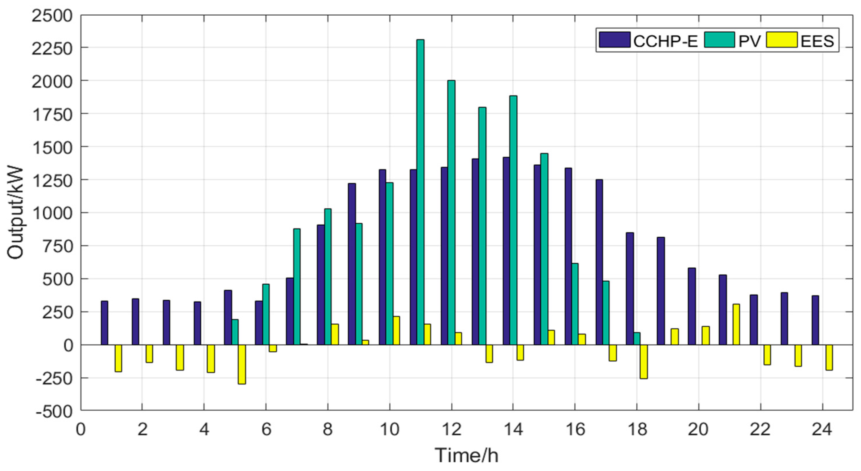
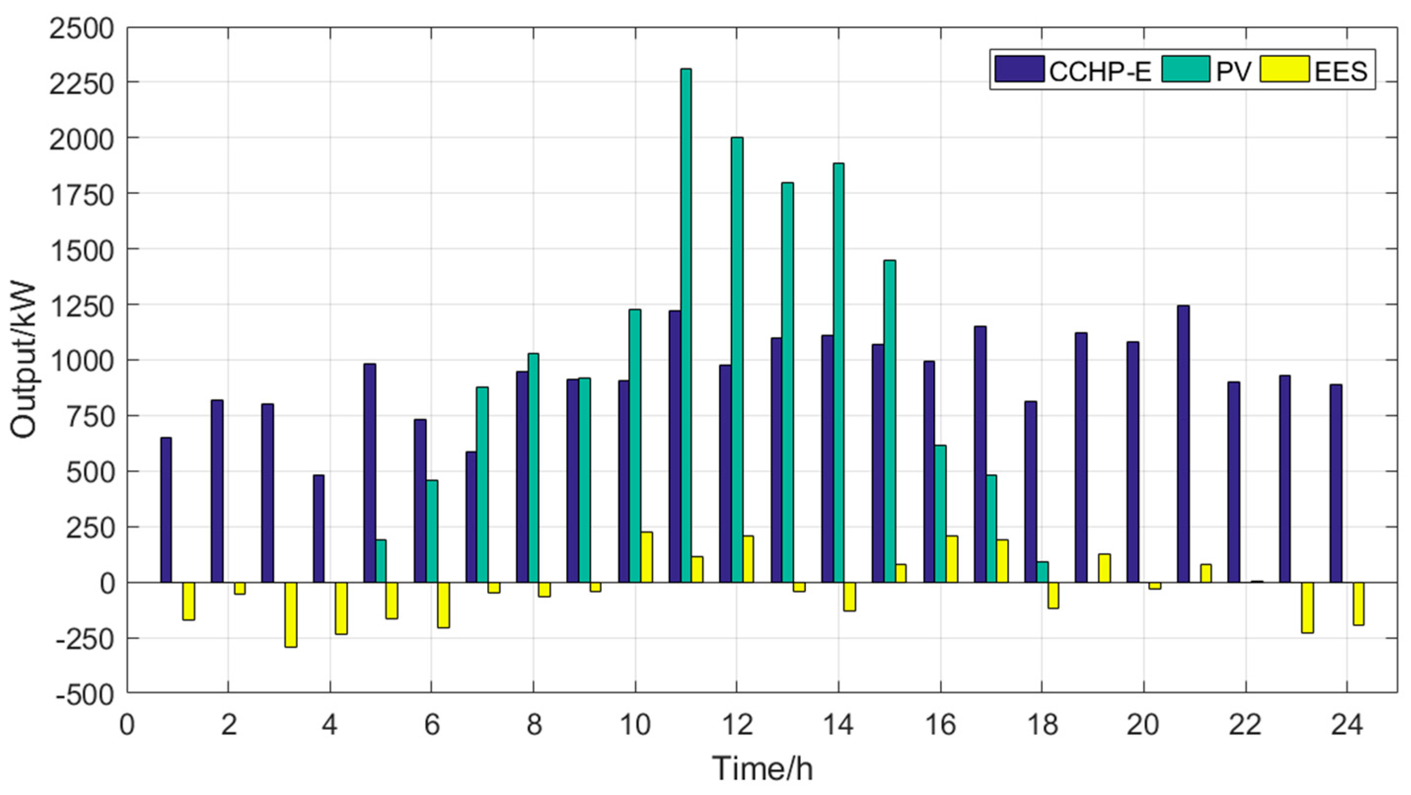
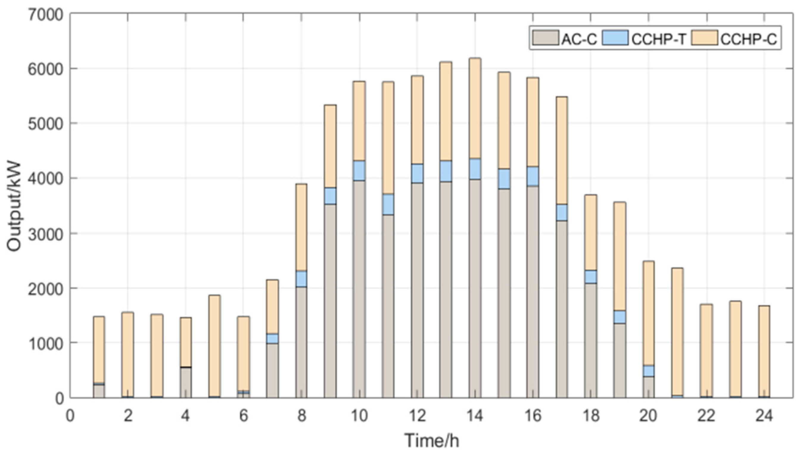
4.2.2. Operation Optimization Result

Figure 10, Figure 11 and Figure 12 show the supply of CCHP, photovoltaic, and energy storage batteries in the power system under three operating modes. A positive EES indicates battery discharge, and a negative EES indicates battery charging. Under the premise of participating in system economic dispatch, EES conducts charging and discharging under the guidance of electricity price, namely, charging and discharging during low and peak periods of electricity price. The current charging and discharging status is determined based on the electricity price and normal period load conditions, thereby effectively reducing the peak valley difference between power load and thermal load.

Mode 1 does not consider the cooperative relationship of each energy supply entity and only takes the optimization goal of the day-ahead scheduling as the solution goal of the model. Therefore, the output strategy of each energy supply entity is the optimal scheduling scheme of the system under the solution goal. From Figure 10, it can be seen that the electrical output of the CCHP system follows the changes in electrical load, and the energy storage system charges and discharges based on electricity prices.

Mode 2 considers the cooperative relationships of various energy supply entities based on comprehensive marginal contributions and formulates operational strategies while maximizing the interests of the cooperating entities. From Figure 11, it can be seen that the electrical output of the CCHP system is affected by the entire energy supply system, and the output is stable. The charging and discharging strategy of the energy storage system is influenced by electricity prices, loads, and the output of other equipment in the system in order to maximize the benefits of the cooperative alliance.

Mode 3 considers the difference between the day-ahead scheduling scheme and the daily output and optimizes and adjusts the actual output of the VPP in time to meet the output of the day-ahead scheduling scheme as much as possible. According to Figure 12, the CCHP system output in Mode 3 shows a similar trend to that in Mode 2. The energy storage system is not only subject to the scheduling of the previous optimization plan but also needs to use the remaining capacity to adjust the load deviation.

Due to the small installed capacity of distributed power generation, all three modes rely heavily on the power grid. The total daily electricity consumption in mode 2 is 145.617 MWh, the total daily electricity consumption in mode 2 is 132.962 MWh, and the total daily electricity consumption in mode 3 is 138.719 MWh. All three modes exhibit varying degrees of load deviation.

Figure 13 and Figure 14 show the outputs of each unit of the cooling and heating modules in the system under mode 1 and mode 3 operation modes, including the combined cooling, heating, and power generation unit and distributed refrigeration unit. In both modes, the heat demand is mainly met by CCHP units, while the cold demand is mainly met by CCHP and electric refrigeration units. Compared with Mode 1, Mode 3 has less dependence on the refrigerator, increasing the output of the CCHP unit and reducing electricity consumption.

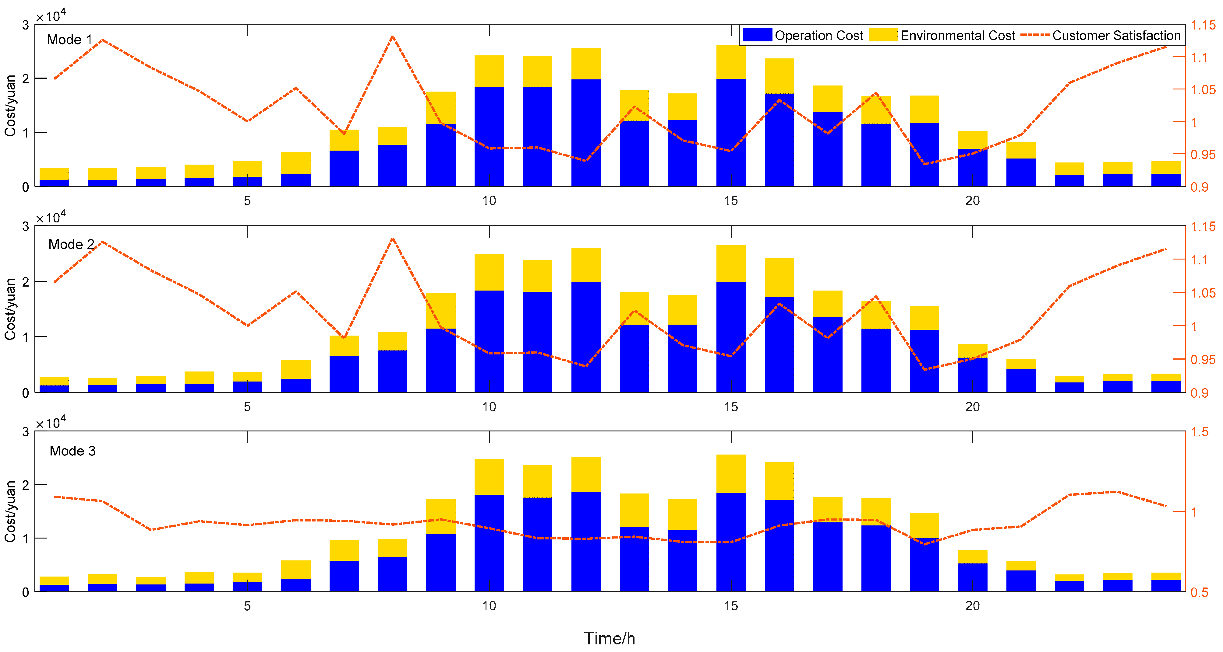
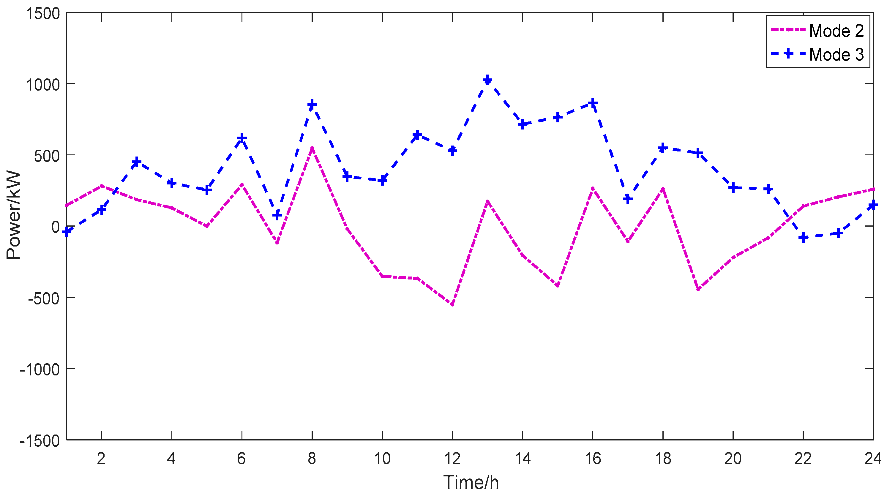
4.3. Discussion and Analysis

Table 4. Daily operating costs.

	Mode 1	Mode 2	Mode 3
Operating cost	209,039.91	206,117.21	197,026.26
Environmental costs	97,503.24	89,355.094	93,157.18

shows the total operating and environmental cost data for a scheduling day. Compared to Mode 1, Mode 2 and Mode 3 have relatively lower operating and environmental costs. Mode 3 reduced operating costs by 5.75% and environmental costs by 4.46%. In the two-stage operation mode, in order to meet the energy supply demand, the power output of equipment with high pollution emissions has been increased. Therefore, the environmental cost of Mode 3 is higher than that of Mode 2.

To measure the impact of DR on user energy consumption, this section introduces the concept of customer satisfaction. Customer satisfaction is the ratio of the load after DR to the load before DR. When customer satisfaction is greater than 1, it indicates that the load after DR is greater than the load before DR. On the contrary, it means that the load after DR is less than the load before DR. Figure 15 shows the operating cost, environmental cost, and customer satisfaction curves for a scheduling day under three modes. The overall operating and environmental costs follow the load curve. Mode 1 is a non-cooperative optimization operation mode, resulting in the highest daily operating and environmental costs. Compared with Mode 1, Mode 2 operates in a collaborative optimization manner, resulting in a relatively lower operating cost and the lowest environmental cost. Mode 3 has the lowest daily operating cost and the best social benefits, but in order to complete the second stage optimization task, the environmental cost has increased compared to Mode 2.

Table 5. Profit and Distribution under Different Modes.

Mode	Mode 1	Mode 2	Mode 3
Total profit	8561.31	10,345.58	11,088.67
PV	1802.45	2345.67	2571.95
CCHP	2120.38	3814.08	3873.96
EES	1875.28	2194.28	2276.12
AC	1763.2	1991.55	2366.64

shows the distribution of profits under different modes. Overall, the profit of the model proposed in this article is the highest. Compared with Mode 1, the profit obtained by PV in Mode 3 increased by 42.69%, and the proportion of profit distribution by PV increased by 2.14%. In addition, the profit distribution proportion of CCHP in Modes 2 and 3 has significantly increased compared to Mode 1. Figure 16 shows the load curve after demand response under mode 2 and mode 3 operating modes. Figure 17 shows the demand response curve under mode 2 and mode 3 operating modes.

From Figure 17, it can be seen that the time of use electricity price adopted in Mode 2 reduces the peak valley difference of household electricity load from 6.88 MW to 6.36 MW, the peak load from 9.12 MW to 8.75 MW, and the minimum load from 2.24 MW to 2.38 MW, effectively shifting the electricity load. Compared with Mode 2, Mode 3 will utilize energy storage devices and user remaining adjustable loads to absorb some electrical energy during certain periods in order to reduce the punishment cost caused by deviant loads.

From Figure 17, it can be seen that Mode 2 adjusts part of the load during peak electricity prices to low electricity price periods, reducing the energy cost of the system. Mode 3 adjusts the load response based on real-time load changes and previous optimizations, reducing the system’s punishment cost and achieving the lowest operating cost within the daily scheduling cycle.

Figure 18 shows the punishment cost changes of deviant loads during the daily scheduling cycles of Mode 2 and Mode 3. Figure 19 shows the variation of deviation load during the daily scheduling cycle of Mode 2 and Mode 3. From 9:00 to 16:00, due to the increase in real-time load compared to the previous forecast data, modes 2 and 3 both experienced varying degrees of power shortages and punishment costs.

From Figure 18 and Figure 19, it can be seen that Mode 2 does not consider real-time load changes, with an average load deviation of 5.22%. Mode 3 utilizes energy storage equipment and remaining adjustable loads to reduce the average deviation load to 2.94%, which to some extent reduces the deviation load and its punishment costs, thereby reducing the daily operating cost of the system.

In order to further analyze the impact of parameter changes on the model proposed in this article, this section conducted sensitivity analysis of deviation punishment changes and DR rewards. This section investigates the impact of different deviation punishment costs and DR rewards on the operation results of the proposed model and the VPP and selects different scenarios in Modes 2 and 3 for calculation and analysis. Figure 20 shows the impact of deviation punishment changes on the operating cost of this VPP, while Figure 21 shows the impact of demand response reward changes on the operating cost of this VPP.

From Figure 20, it can be seen that an increase in deviation penalties will lead to an increase in system operating costs. Mode 2 only optimized the energy supply system in one stage, without considering the impact of real-time load changes on deviation costs. Therefore, the energy supply strategy of Mode 2 is not affected by the variation of deviation punishment, and its punishment cost varies proportionally with the variation of deviation punishment. The change in deviation punishment has an impact on the energy supply strategy of Mode 3, mainly on the optimization of two-stage scheduling. When the punishment for deviation increases by 5%, Mode 3 utilizes energy storage equipment and remaining flexible loads to absorb some of the deviation loads, reducing a portion of the increase in operating costs caused by load deviation. When the punishment for deviation increases by 10%, the energy storage equipment and flexible load consumption have reached their maximum capacity, and the punishment cost cannot be reduced by reducing the load deviation. The system operating cost will increase by about 1.8%. The decrease in deviation penalties can also lead to varying degrees of reduction in operating costs.

From Figure 21, it can be seen that an increase in DR rewards will lead to a decrease in system operating costs. In Mode 2, an increase in DR rewards will motivate users to change the energy consumption curve and increase DR. When the DR reward increases by 5%, users will actively respond to demand changes within the adjustable load range, resulting in a 1.82% decrease in operating costs. When the DR reward increases by 10%, the decrease in system operating costs slows down due to the limitation of user’s DR ability. Compared with Mode 2, Mode 3 shows different trends in change. In Mode 3, changes in DR rewards not only affect the user’s DR ability, but also alter the system’s ability to adjust deviations. When the DR reward increases by 10%, users can use adjustable loads to respond to changes in demand while reducing the ability to adjust deviation loads, increasing the cost of deviation penalties, and reducing system operating costs by 1.10%. When the DRS reward is reduced by 10%, users will have more adjustable load to absorb the deviation load, but the system operating cost will increase by 5.54%.

5. Conclusions

In this paper, a two-stage VPP optimization model considering the user-VPP-equipment alliance is proposed. By dividing the VPP into two coalitions: demand-side user-VPP and supply-side equipment-VPP, a VPP optimization framework considering the cooperation game of user-VPP- equipment alliance is established. A two-stage optimization model of VPPs is established. The day-ahead optimization aims at economic benefit and social benefit, and intraday optimization aims at minimizing deviation punishment cost. In addition, the profit distribution method combining the improved Shapley value and the independent risk contribution theory is used to distribute the total income of the VPP. The case results show that the operating cost has been reduced by 5.75%, the environmental cost has been reduced by 4.46%, and the total profit has increased by 29.52%. The model can improve the overall efficiency of VPPs. Sensitivity analysis shows that changes in punishment costs within the range of ±5% have little impact on operating costs, and an increase in DR incentive intensity will reduce the operating costs of VPP. However, the research in this paper does not involve the internal interaction between multiple VPPs and the game behavior, which will be the next research focus.

References

1. Gazijahani, F.S.; Salehi, J. IGDT-based complementarity approach for dealing with strategic decision making of price-maker VPP considering demand flexibility. IEEE Trans. Ind. Inform. 2019, 16, 2212–2220. [Google Scholar] [CrossRef]
2. Peake, S. Renewable Energy-Power for a Sustainable Future; Oxford University Press: Oxford, UK, 2018. [Google Scholar]
3. Pepermans, G.; Driesen, J.; Haeseldonckx, D.; Belmans, R.; D’haeseleer, W. Distributed generation: Definition, benefits and issues. Energy Policy 2005, 33, 787–798. [Google Scholar] [CrossRef]
4. Johansson, P.-O.; Kriström, B. Welfare evaluation of subsidies to renewable energy in general equilibrium: Theory and application. Energy Econ. 2019, 83, 144–155. [Google Scholar] [CrossRef]
5. Yu, S.; Fang, F.; Liu, Y.; Liu, J. Uncertainties of virtual power plant: Problems and countermeasures. Appl. Energy 2019, 239, 454–470. [Google Scholar] [CrossRef]
6. Kumagai, J. Virtual power plants, real power. IEEE Spectr. 2012, 49, 13–14. [Google Scholar] [CrossRef]
7. Chu, T.; An, X.; Zhang, W.; Lu, Y.; Tian, J. Multiple Virtual Power Plants Transaction Matching Strategy Based on Alliance Blockchain. Sustainability 2023, 15, 6939. [Google Scholar] [CrossRef]
8. Kasaei, M.J.; Gandomkar, M.; Nikoukar, J. Optimal management of renewable energy sources by virtual power plant. Renew. Energy 2017, 114, 1180–1188. [Google Scholar] [CrossRef]
9. Li, Q.; Wei, F.; Zhou, Y.; Li, J.; Zhou, G.; Wang, Z.; Liu, J.; Yan, P.; Yu, D. A scheduling framework for VPP considering multiple uncertainties and flexible resources. Energy 2023, 282, 128385. [Google Scholar] [CrossRef]
10. Liu, J.; Yu, S.S.; Hu, H.; Trinh, H. A combinatorial auction energy trading approach for VPPs consisting of interconnected microgrids in demand-side ancillary services market. Electr. Power Syst. Res. 2023, 224, 109694. [Google Scholar] [CrossRef]
11. Gulotta, F.; del Granado, P.C.; Pisciella, P.; Siface, D.; Falabretti, D. Short-term uncertainty in the dispatch of energy resources for VPP: A novel rolling horizon model based on stochastic programming. Int. J. Electr. Power Energy Syst. 2023, 153, 109355. [Google Scholar] [CrossRef]
12. Zhang, T.; Qiu, W.; Zhang, Z.; Lin, Z.; Ding, Y.; Wang, Y.; Wang, L.; Yang, L. Optimal bidding strategy and profit allocation method for shared energy storage-assisted VPP in joint energy and regulation markets. Appl. Energy 2023, 329, 120158. [Google Scholar] [CrossRef]
13. Yang, C.; Du, X.; Xu, D.; Tang, J.; Lin, X.; Xie, K.; Li, W. Optimal bidding strategy of renewable-based virtual power plant in the day-ahead market. Int. J. Electr. Power Energy Syst. 2023, 144, 108557. [Google Scholar] [CrossRef]
14. Guo, W.; Liu, P.; Shu, X. Optimal dispatching of electric-thermal interconnected virtual power plant considering market trading mechanism. J. Clean. Prod. 2021, 279, 123446. [Google Scholar] [CrossRef]
15. Wang, Y.; Wu, X.; Liu, M.; Zhang, C.; Wang, H.; Yue, Y.; Luo, X. Bidding strategy of the virtual power plant considering green certificates and carbon trading. Energy Rep. 2023, 9, 73–84. [Google Scholar] [CrossRef]
16. Mei, S.; Tan, Q.; Liu, Y.; Trivedi, A.; Srinivasan, D. Optimal bidding strategy for virtual power plant participating in combined electricity and ancillary services market considering dynamic demand response price and integrated consumption satisfaction. Energy 2023, 284, 128592. [Google Scholar] [CrossRef]
17. Nokandi, E.; Vahedipour-Dahraie, M.; Goldani, S.R.; Siano, P. A three-stage bi-level model for joint energy and reserve scheduling of VPP considering local intraday demand response exchange market. Sustain. Energy Grids Netw. 2023, 33, 100964. [Google Scholar] [CrossRef]
18. Cao, J.; Zheng, Y.; Han, X.; Yang, D.; Yu, J.; Tomin, N.; Dehghanian, P. Two-stage optimization of a virtual power plant incorporating with demand response and energy complementation. Energy Rep. 2022, 8, 7374–7385. [Google Scholar] [CrossRef]
19. Liu, H.; Wang, C.; Ju, P.; Xu, Z.; Lei, S. A bi-level coordinated dispatch strategy for enhancing resilience of electricity-gas system considering virtual power plants. Int. J. Electr. Power Energy Syst. 2023, 147, 108787. [Google Scholar] [CrossRef]
20. Fang, F.; Yu, S.; Liu, M. An improved Shapley value-based profit allocation method for CHP-VPP. Energy 2020, 213, 118805. [Google Scholar] [CrossRef]
21. Wang, X.; Li, B.; Wang, Y.; Lu, H.; Zhao, H.; Xue, W. A bargaining game-based profit allocation method for the wind-hydrogen-storage combined system. Appl. Energy 2022, 310, 118472. [Google Scholar] [CrossRef]
22. Rahmani-Dabbagh, S.; Sheikh-El-Eslami, M.K. A profit sharing scheme for distributed energy resources integrated into a virtual power plant. Appl. Energy 2016, 184, 313–328. [Google Scholar] [CrossRef]
23. Cremers, S.; Robu, V.; Hofman, D.; Naber, T.; Zheng, K.; Norbu, S. Efficient methods for approximating the Shapley value for asset sharing in energy communities. In Proceedings of the Thirteenth ACM International Conference on Future Energy Systems, Virtual, 28 June–1 July 2022. [Google Scholar]
24. Wang, Y.; Liu, Z.; Cai, C.; Xue, L.; Ma, Y.; Shen, H.; Chen, X.; Liu, L. Research on the optimization method of integrated energy system operation with multi-subject game. Energy 2022, 245, 123305. [Google Scholar] [CrossRef]
25. Yang, J. Transaction decision optimization of new electricity market based on virtual power plant participation and Stackelberg game. PLoS ONE 2023, 18, e0284030. [Google Scholar] [CrossRef] [PubMed]
26. Wu, H.; Liu, X.; Ye, B.; Xu, B. Optimal dispatch and bidding strategy of a virtual power plant based on a Stackelberg game. IET Gener. Transm. Distrib. 2020, 14, 552–563. [Google Scholar] [CrossRef]
27. Gougheri, S.S.; Dehghani, M.; Nikoofard, A.; Jahangir, H.; Golkar, M.A. Economic assessment of multi-operator virtual power plants in electricity market: A game theory-based approach. Sustain. Energy Technol. Assess. 2022, 53, 102733. [Google Scholar] [CrossRef]
28. Zhou, J.; Chen, K.; Wang, W. A Power Evolution Game Model and Its Application Contained in Virtual Power Plants. Energies 2023, 16, 4373. [Google Scholar] [CrossRef]
29. Wang, Y.; Wang, Y.; Huang, Y.; Yang, J.; Ma, Y.; Yu, H.; Zeng, M.; Zhang, F.; Zhang, Y. Operation optimization of regional integrated energy system based on the modeling of electricity-thermal-natural gas network. Appl. Energy 2019, 251, 113410. [Google Scholar] [CrossRef]
30. Wang, Y.; Ma, Y.; Song, F.; Ma, Y.; Qi, C.; Huang, F.; Xing, J.; Zhang, F. Economic and efficient multi-objective operation optimization of integrated energy system considering electro-thermal demand response. Energy 2020, 205, 118022. [Google Scholar] [CrossRef]
31. Liu, R.; Zhao, Z.; Sun, G.; Mi, Y.; Pan, Z. Optimization strategy and profit allocation of virtual power plant considering different risk preference. Electr. Power Autom. Equip. 2021, 41, 154–161. [Google Scholar]
Figure 1. Basic Structure of VPP.
Sustainability 15 13960 g001
Figure 2. Optimization framework of VPP considering alliance cooperation game of user-VPP-equipment.
Sustainability 15 13960 g002
Figure 3. VPP two-stage optimization framework considering multi-agent cooperative games.
Sustainability 15 13960 g003
Figure 4. Flow chart of the NSGA-II based on day-ahead optimal scheduling model.
Sustainability 15 13960 g004
Figure 5. Typical curves of daily power load, thermal load, and cooling load.
Sustainability 15 13960 g005
Figure 6. Renewable energy output curve.
Sustainability 15 13960 g006
Figure 7. Daily variation curve of electricity price and natural gas price.
Sustainability 15 13960 g007
Figure 8. Fitness curve of NSGA-Ⅱ in different stages of Mode 3.
Sustainability 15 13960 g008
Figure 9. CPU usage and runtime graph of NSGA-Ⅱ in different stages of Mode 3.
Sustainability 15 13960 g009
Figure 10. Power Supply Equipment Output Strategy for Mode 1.
Sustainability 15 13960 g010
Figure 11. Output Strategy of Power Supply Equipment in Mode 2.
Sustainability 15 13960 g011
Figure 12. Output Strategy of Power Supply Equipment in Mode 3.
Sustainability 15 13960 g012
Figure 13. Output of the hot and cold system in mode 1.
Sustainability 15 13960 g013
Figure 14. Output of the hot and cold system in mode 3.
Sustainability 15 13960 g014
Figure 15. Daily operating costs, environmental costs, and customer satisfaction under different modes.
Sustainability 15 13960 g015
Figure 16. Load Curve after Demand Response in Modes 2 and 3.
Sustainability 15 13960 g016
Figure 17. Variation of electric load before and after demand response.
Sustainability 15 13960 g017
Figure 18. Punishment Costs for Modes 2 and 3.
Sustainability 15 13960 g018
Figure 19. Deviation Load Changes in Modes 2 and 3.
Sustainability 15 13960 g019
Figure 20. Sensitivity Analysis Curve of punishment cost.
Sustainability 15 13960 g020
Figure 21. Sensitivity Analysis Curve of demand response incentive.
Sustainability 15 13960 g021