Flow Turbulence and Pressure Fluctuations in a Hydraulic Jump

Abstract

Turbulence and pressure fluctuations are key elements in the bed protection design of hydraulic structures. However, their roles in a hydraulic jump are not yet fully understood, and the nature of their relationships are not conclusive. In order to better understand the relationships between pressure fluctuations and flow characteristics of a hydraulic jump downstream of a weir, detailed measurements of flow kinematics using the nonintrusive techniques of particle image velocimetry and bubble image velocimetry and pressure using voltage-type pressure gauges were carried out in this study. The physical modeling of the hydraulic jump was carried out using the simultaneous measurements of pressure and turbulent flow properties. The distributions of flow properties, such as water level and velocity, were assessed in each case. Based on the measurements, the correlations between the pressure fluctuations and the variables were investigated by coupling the statistical values of the variables at the same points. The analysis results show that the water level and turbulence intensity are the main factors influencing the pressure fluctuations in the hydraulic jump. Using these factors, an empirical formula and dimensionless numbers are proposed to show that the pressure fluctuations depend on the bubble flow behavior.

1. Introduction

Riverbed protection has been proposed to stabilize riverbeds against turbulent pressures due to hydraulic jumps that occur downstream of transverse structures such as dams and sluice gates. In general, the design standards for riverbed protection, such as stilling basin bottoms and riprap, are mainly focused on steady state pressures. However, transient pressures can exceed the structural capacity of the riverbed protection designed to prevent bed scour [1,2]. In addition, pressure fluctuations at the bottom and both walls of stilling basins pose a serious risk due to uplift of the basin slab, fatigue, material erosion and cavitation [2,3,4,5]. In such cases, pressure fluctuations can be a critical factor in the safety of hydraulic structures. Therefore, there are some suggestions when considering the risk of pressure fluctuations, which have not been sufficiently investigated in this respect [2,5,6,7]. The American Concrete Institute has emphasized the importance of investigating the fatigue failure of hydraulic structures caused by low amplitude, high frequency cyclic loading [8]. The high frequency loads are relevant to the real component of turbulence. The turbulence in the hydraulic jump is composed of slow flow fluctuations and fast velocity turbulence. Meanwhile, the low-frequency motion in a roller region is due to large vortical structures and free surface fluctuations [5].

The dimensionless index of pressure fluctuations used in previous studies is twofold, including the pressure coefficient ($C_p^{\prime }$) and the maximum and minimum dimensionless pressure fluctuation ($C_p$). The maximum dimensionless pressure fluctuation depends on the Froude number, incident flow development, run time, jump toe position, and chute slope [9,10]. It has also been reported that the pressure fluctuation is mainly related to large-size eddies and their cumulative effects [5,11]. In particular, in a low-shear layer, the high-frequency pressure fluctuations were strongly correlated with the kinetic pressure fluctuations rather than the free surface fluctuations. This result is consistent with that of the frequency analysis of pressure in previous studies: the frequency of pressure in the initial part of the jump is higher than downstream, and the frequency distribution of pressure in the initial part is more skewed and peaked than downstream [9,11,12,13,14]. In addition, free surface fluctuation is related to the oscillations in the position of the jump toe and the entrainment of the air entrapped by the jump toe [15]. Overall, there is a complex interaction between the following hydraulic factors: (1) free surface fluctuations, (2) changes in fluid density due to bubble movement and diffusion, (3) changes in dynamic pressure due to impinging flow near the bottom, and (4) changes in eddy structures, which can affect pressure fluctuations. These variables influence each other directly and indirectly, resulting in complex phenomena. As a result, it is not easy to quantitatively assess the effect of each variable on pressure fluctuations.

Early studies were mainly carried out under weak jump conditions with a relatively low void fraction as the high void fraction makes it difficult to measure the flow properties such as water level and velocity. However, recent studies have used non-intrusive techniques such as laser Doppler velocimetry (LDV), light detection and ranging (LIDAR), and particle image velocimetry (PIV) to measure turbulent flow properties [16,17,18,19]. In particular, many studies have used PIV measurements at the jump because PIV has several advantages over non-intrusive techniques. It is more accurate and can measure the velocity distribution over a section rather than at a single given point, which is useful for elucidating the characteristics of roller regions [15,19,20]. Furthermore, Lin et al. [20] used PIV and bubble image velocimetry (BIV) to investigate the turbulent flow properties and the flow structure in a steady hydraulic jump as BIV is suitable for measuring bubble flow. They showed that the bubble and water velocities were almost equal or constant, depending on the Reynolds stress.

Based on the need for further studies on the flow kinematic factors affecting the pressure fluctuations of the hydraulic jump, this study investigates the quantitative relationships between the pressure pattern and flow kinematics through physical modeling tests over the downstream field of a weir. Since the pressure fluctuation pattern is expected to directly affect the structural stability of the bed downstream of a weir, understanding the pressure changes as a function of flow conditions is of significant importance in terms of bed stability and weir design. The specific objectives of the present study are as follows:

(1)

To quantify the spatial variations in the flow characteristics and pressure fluctuation distribution under hydraulic jump flow conditions;

(2)

To determine the relationship between flow property variables (horizontal and vertical velocities, horizontal and vertical turbulence intensities, water level, and water level fluctuation) and pressure fluctuation;

(3)

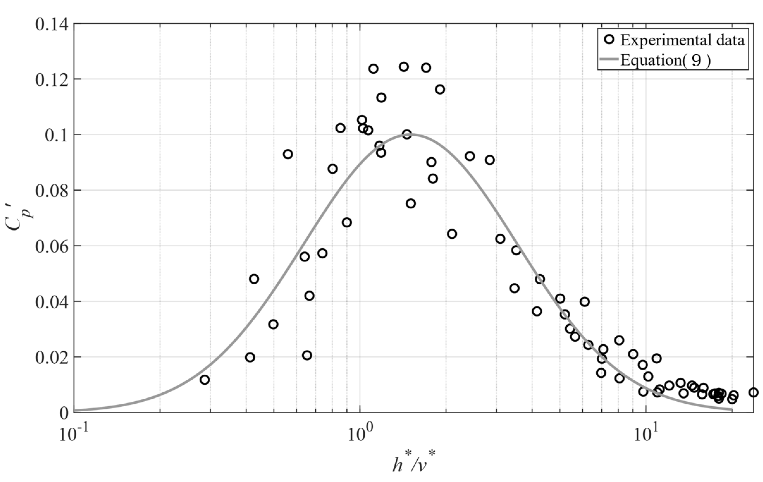
To propose an empirical formula for estimating the pressure fluctuation coefficient at the bottom of the structure using dimensionless numbers.

This paper is organized as follows. Section 1 presents a literature reviews of previous studies related to hydraulic jump flows. Section 2 provides a detailed explanation of the experiments, including the setup and conditions, as well as the measurement methods. Section 3 presents and explains the results obtained from the measurements and analysis, focusing on the patterns of the flow parameters and the relationships between them. The interpretation of the results is discussed in Section 4. Section 5 concludes the paper.

2. Materials and Methods

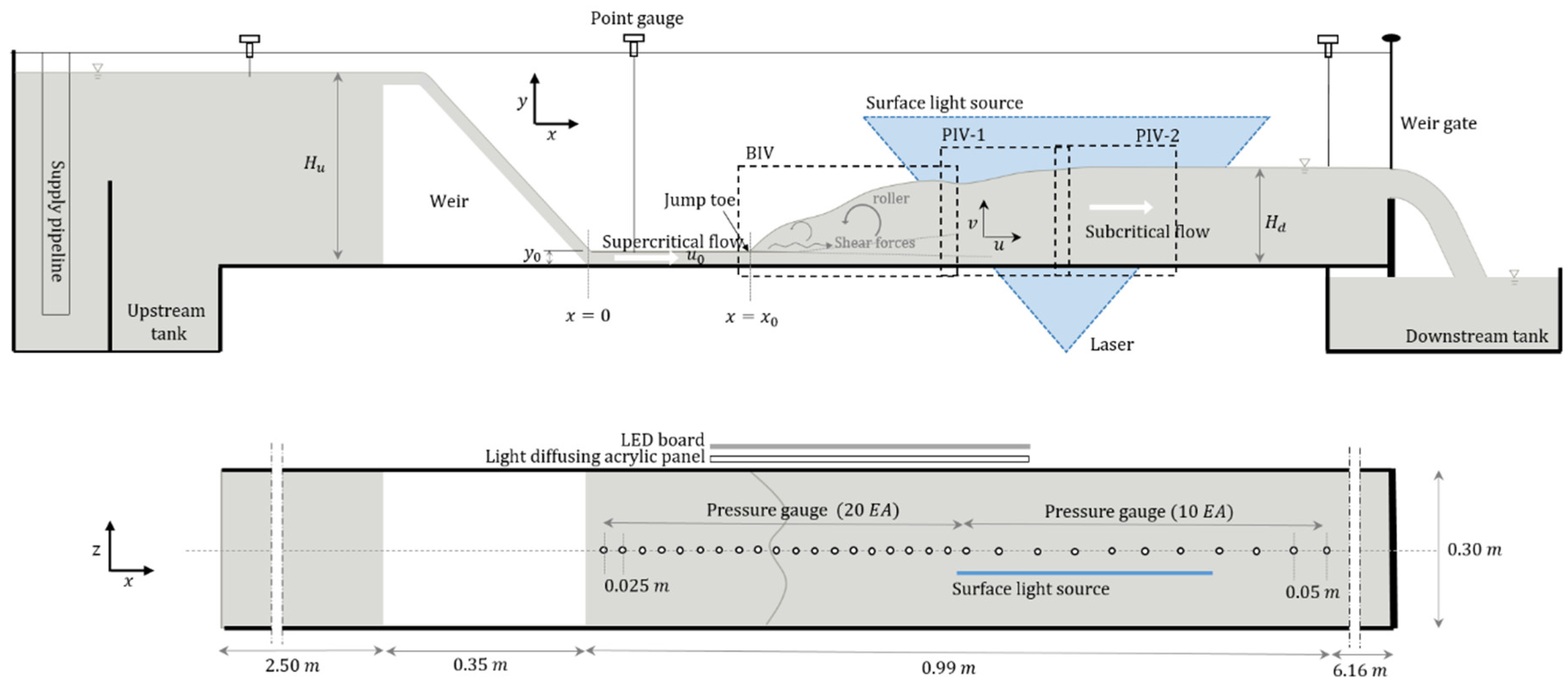
2.1. Experimental Setup and Conditions

The experiments were performed in a circular experimental channel equipped with a pump with a maximum capacity of 0.0063 ${\mathrm{m}}^3/\mathrm{s}$; the channel was 10 m long, 0.3 m wide, and 0.45 m high (Figure 1). Both sides and the bottom of the channel were made of tempered glass for facilitating optical measurements. A fixed weir made of acrylic material with a front slope of 1:1 and a height of 0.3 m was installed 2.5 m downstream of the upstream inflow section. A weir-type gate was installed to regulate the downstream water level at 7.15 m from the toe of the weir and the water cascaded freely into the outflow water tank.

In order to investigate the turbulent flow fields and pressures in the hydraulic jump, the hydraulic experiments were carried out under six different conditions by adjusting the downstream water level and inflow discharge (

Table 1. Experimental cases.

Case	Discharge (m3/s)	Hu (m)	Hd (m)	y0 (m)	u0 (m/s)	x0 (m)	$\mathit{F}\mathbf{r}$ ($=\frac{{\mathit{u}}_0}{\sqrt{\mathit{g}{\mathit{y}}_0}}$)	$\mathit{R}\mathbf{e}$ ($=\frac{{\mathit{u}}_0{\mathit{y}}_0}{\mathit{\nu }}$)
1	0.0063	0.355	0.0900	0.0085	2.47	0.125	8.6	$2.1\times {10}^4$
2			0.0893			0.216
3	0.0047	0.347	0.0766	0.0078	2.01	0.125	7.3	$1.6\times {10}^4$
4			0.0754			0.214
5	0.0035	0.338	0.0604	0.0068	1.71	0.280	6.6	$1.2\times {10}^4$
6	0.0019	0.327	0.0355	0.0053	1.19	0.365	5.2	$6.3\times {10}^3$

). The discharge was controlled by a pump flow meter and calibrated before the experiments. The jump toe position ($x_0$) depended sensitively on the water level at the downstream gate. Based on the velocity ($u_0$) and water level ($y_0$) of the incoming supercritical flow before the jump, the conditions used for the experiments corresponded to Froude numbers (Fr) = 5.2–8.6 and Reynolds numbers (Re) = $6.3\times {10}^3 – 2.1\times {10}^4$. In the incoming supercritical flow, a point gauge was used to measure the water level, and the velocity was calculated from the flow measured using a pump flow meter and the measured water level.

2.2. Measurement Method

Pressure, velocity, and water level were measured under the experimental conditions for hydraulic jump flows. To achieve the goal of this study to investigate the patterns and relationships of the properties, the simultaneous and synchronized measurements were conducted. Image-based velocimetry using high speed cameras for the flow velocity and water level was used for the temporal and spatial statistical analysis of the turbulent flows. In particular, the flow fields were measured separately depending on the presence of bubbles. For the temporal variation of the fluctuating pressure on the bed, a time series of pressure data was obtained from pressure gauges.

To investigate the velocity fields in the hydraulic jump, the non-intrusive imaging techniques, PIV and BIV, were used. The BIV method was used to measure the flow properties in the roller region while the PIV method was used to measure those after the jump. In particular, the PIV and BIV methods were used separately depending on the presence of air bubbles. PIV was employed for the measurements in the bubble-free flow region mainly downstream of the hydraulic jump. In contrast, BIV based on the shadowgraphy approach was used for the velocity measurements in the region of the hydraulic jump where bubbles were entrained. This approach was chosen because a laser cannot be used due to light scattering and refraction in a roller region caused by the air–water interface due to water drops, free surfaces, and air bubbles. BIV measures the velocity field through the same principle as PIV; however, BIV measures the velocity through the transfer of the air–water interface instead of using tracer particles. More details on BIV can be found in Ryu et al. [21].

The equipment used for the PIV measurements consisted of two high-speed cameras, tracer particles, and a laser. Although the camera was capable of recording up to 2000 images per second at the full frame, it was set at 500 to 1000 frames per second to obtain 50 velocity fields in 1 s, taking into account the characteristics of turbulent flow. The images of the PIV measurement section were acquired with two high-speed cameras downstream of the hydraulic jump (PIV sections 1 and 2 shown in Figure 1). Particles (silver-coated hollow glass spheres) with the specific gravity of 1.02 and a mean diameter of 40 μm were used as the tracers. The laser, which enables the particles to reflect light for visualization, had a maximum power of 8.0 W. Specifically, the continuous laser was used together with a signal generator to facilitate the adjustments. The laser light was transmitted from the channel bottom so that it was incident on the x–y plane where the velocity field was observed (Figure 1). The line of the laser light sheet was located 1 cm from the channel centerline due to the holes for the pressure measurement.

For measuring the water level at the jump, wave gauges such as wire gauges and ultrasonic sensors have generally been used due to their advantages in observing the instantaneous water level; however, these measurements can be affected by splashes and droplets [22,23]. Therefore, in this study, the images taken for the velocity measurements were also used for the water level measurements. This approach is analogous to the method used by Nóbrega et al. [23]. The accuracies were 0.09 and 0.2 $\mathrm{m}\mathrm{m}/\mathrm{p}\mathrm{x}$ for PIV and BIV region images, respectively. By digitizing the images taken at each time point, the water level was extracted based on the pixel values (I(x, y)), which ranged from 0 (dark value) to 255 (bright value). In the BIV images, the difference in brightness depended on the bubble content or water–air interface and the free surface tended to be the darkest at each vertical column. Therefore, the point where the value of a specific pixel was smaller (darker) than the upper and lower averages was identified as the water level as follows:

$$I\left(x,y=\eta \right)<\alpha \overline{I(x,y>\eta )}$$

(1)

$$I\left(x,y=\eta \right)<\beta \overline{I(x,y<\eta )}$$

(2)

where $I$ is the pixel value of the image; $x$ and $y$ are the coordinates in the flow and vertical directions, respectively; $\alpha$ and $\beta$ denote the coefficients; and $\eta$ represents the water level. In addition, the coefficients were manually modified considering the characteristics of the images, including brightness, depending on the experimental conditions. The manual data processing ensured maximum reliability of the results. Figure 2 presents the transient water levels obtained using the images from the BIV measurements. Despite the strong free surface fluctuations in the jump, it was suitable for tracking the water surface profile. The coefficients in Equations (1) and (2) had to be modified because large errors could have occurred due to light scattering and brightness variations. The water level measured in this way was pre-verified by comparing it with the water level measured with a point gauge during the experiments.

Unlike the pressure and PIV velocity measured near the centerline of the channel, the instantaneous velocity and water level from the BIV images were measured near the wall. Fully two-dimensional flows cannot be generated due to discontinuities in the models or unsmoothed channel, energy loss, or reflected waves from the wall effect. Fiorotto and Rinaldo [9] assumed that the statistical properties of the pressure fluctuations are independent of the transverse direction since a transverse correlation is larger than a longitudinal correlation. Therefore, it can be assumed that the relationship between the statistical properties of the pressure fluctuations and the flow properties measured along two parallel lines can be established.

A voltage-type pressure gauge capable of measuring pressure in the range of −2 to 5 kPa and with an accuracy of ±0.04% was used. For the pressure measurements, 30 points were drilled in the channel bottom with 5-mm-diameter circular holes at 2.5 cm intervals for 20 points from the weir toe and at 5 cm intervals for ten points beyond (Figure 1). The holes drilled in the channel bottom and the pressure gauge were connected via an acrylic tube. One hundred pressure readings per second were acquired after the jump flow was sufficiently stabilized, and each measurement was performed for 200 s.

For the flow analysis with the highly turbulent nature, the turbulence intensity of the flow velocity and the pressure fluctuation coefficient were investigated in this study. The turbulence intensity was calculated using the root mean square (RMS) values of the difference between the instantaneous and time-averaged velocities, denoted as $u_{rms}$:

$$u_{rms}=\sqrt{\sum _{t=1}^T{(u_t-\overline{u})}^2/T }$$

(3)

where $u_t$ is the instantaneous velocity, $\overline{u}$ denotes the velocity time average, and T is the total observation time. The pressure fluctuation coefficient was represented by the root mean square divided by the kinetic energy of the incoming supercritical flow [1], denoted as $C_p^{\prime }$.

$$C_p^{\prime }=P_{rms}/(\alpha u_0^2/2g)$$

(4)

In the equation, $\alpha$ is the coefficient, $u_0$ is the velocity of the incoming supercritical flow, and $g$ is the gravitational acceleration.

3. Results

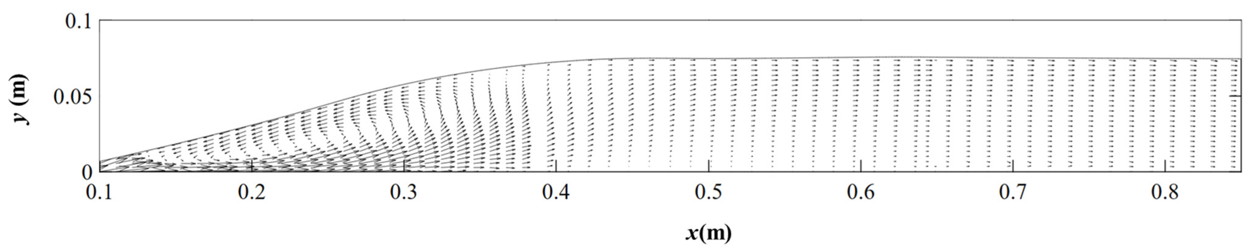
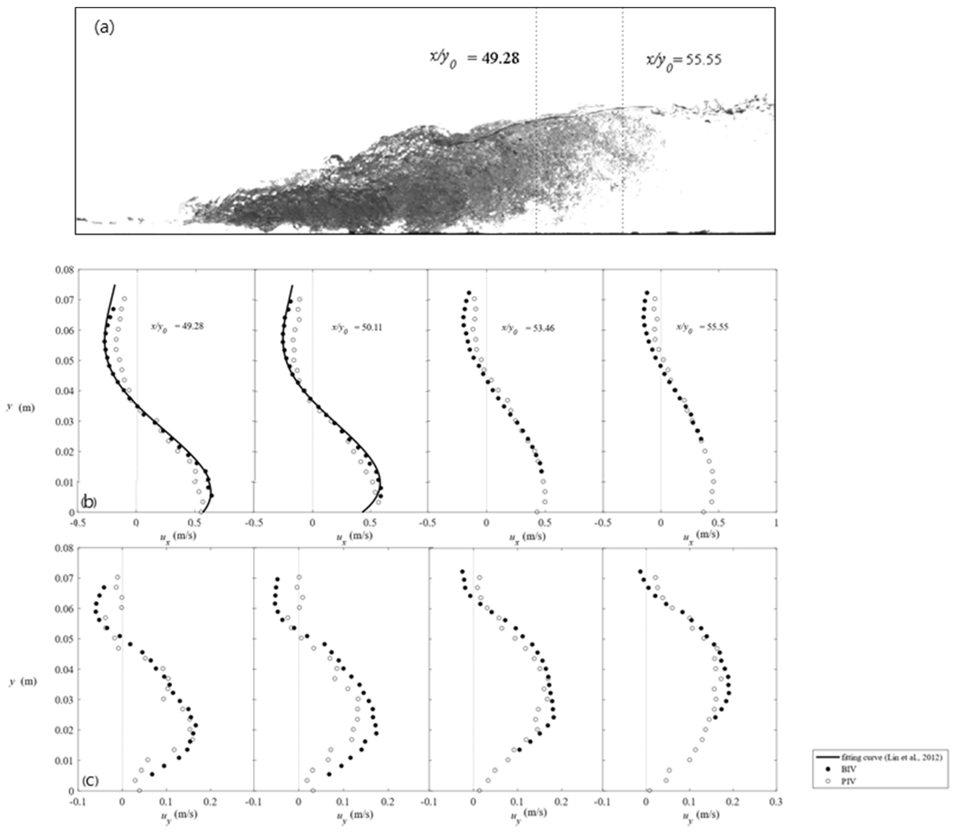
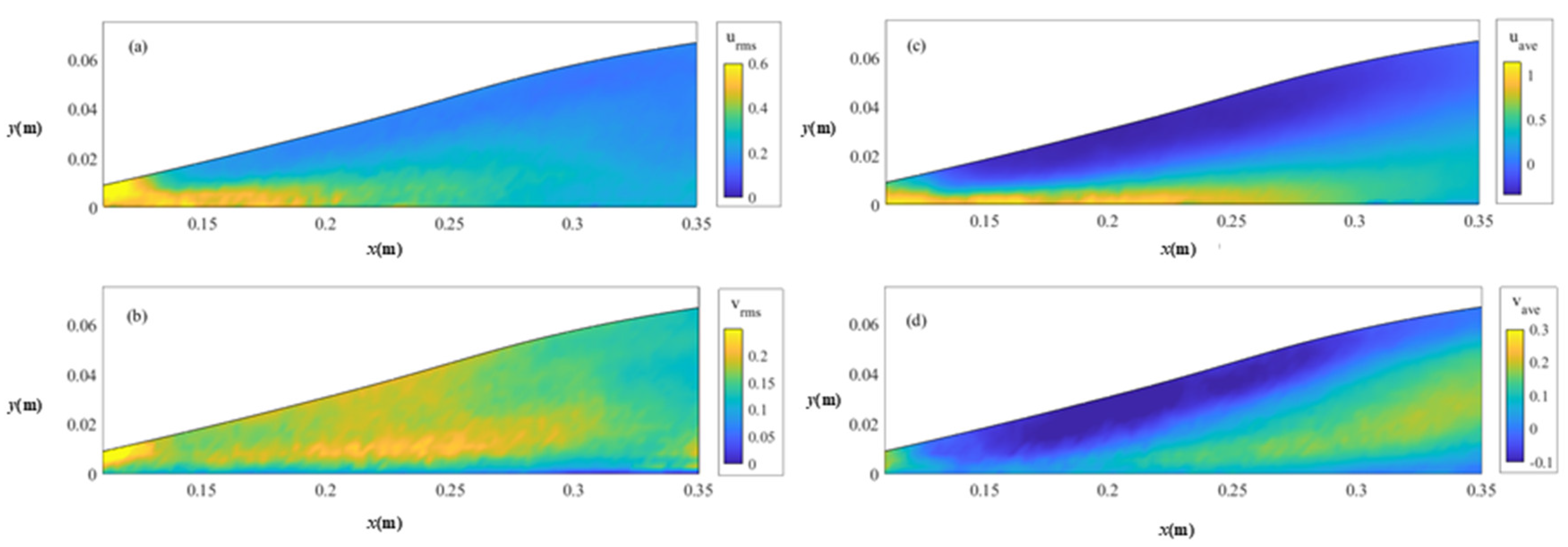
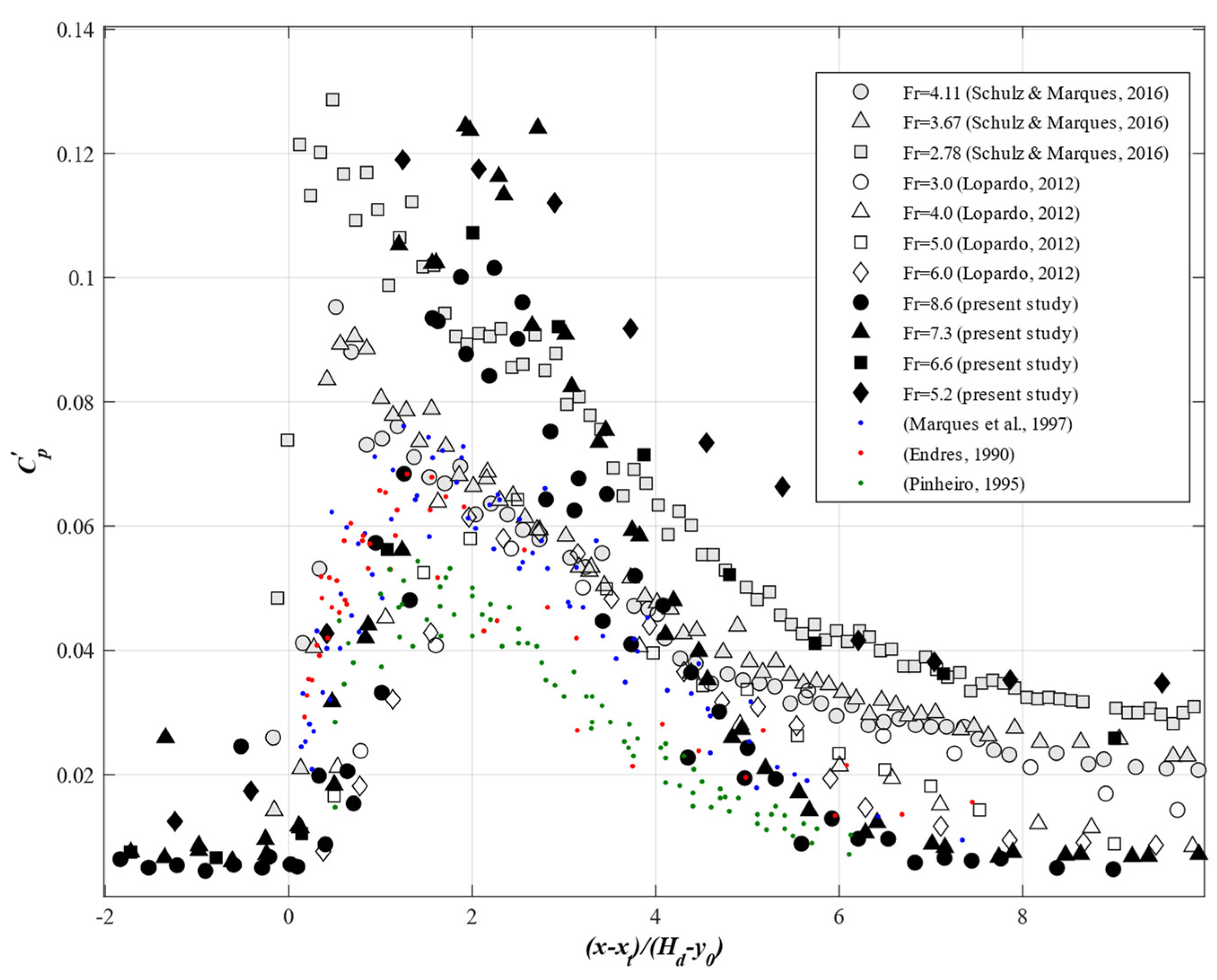
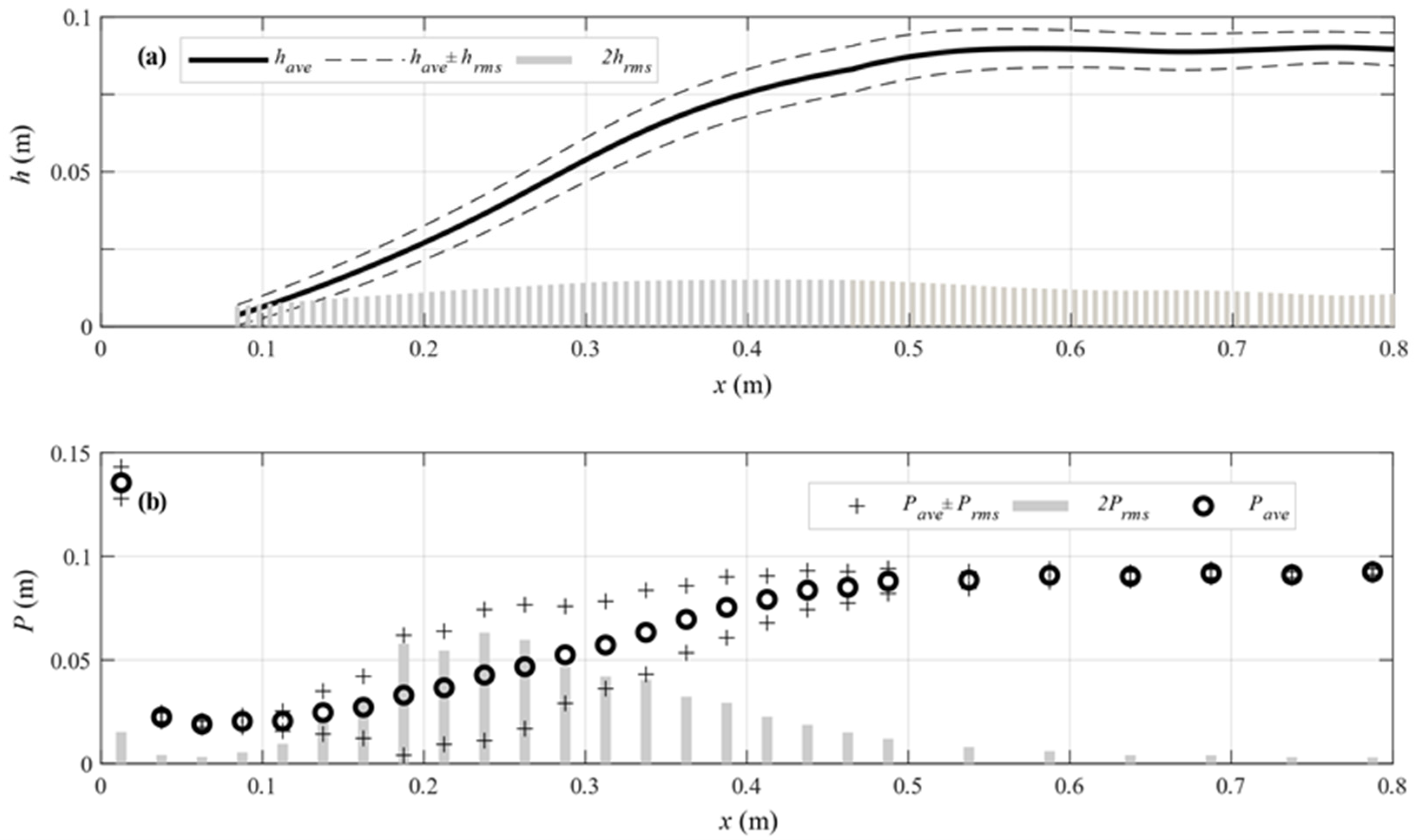
3.1. Validation of Velocity, Water Level, and Pressure Distribution

To measure the complex flow fields of the hydraulic jump, BIV was used at the jump with significant flow aeration while PIV was used for the measurements downstream of the hydraulic jump. The velocity vectors were calculated using PIVlab in MATLAB [24,25] and the outliers were excluded using a standard deviation filter (n = 1). For the velocity vector extraction, the interrogation window size was set to 32 × 32 pixels with 50 % overlap (16 pixels) in the horizontal and vertical directions. The resolutions of PIV and BIV were $∆x=∆y=$ 3.2 and 6.0 mm, respectively. Figure 3 shows the time-averaged velocity vectors to investigate the structure of the hydraulic jump which was investigated in previous studies [5,26].

Figure 4 shows the overlapping data from BIV and PIV to validate the consistency of the two methods. The BIV data became shorter with respect to the distance from the jump toe because there was the sporadic bubble flow in the terminal part of the jump. The velocities measured by the two different methods are almost congruent, although the absolute values are slightly larger for BIV. The difference between the velocities is probably due to the intermittent inflow of the bubble in the overlapping area. The horizontal oscillations of the jump may cause a phenomenon where the slightly higher velocity is observed in the air–water flow region as the toe moves downstream.

The BIV data were also compared with the empirical equation of the bubble velocity proposed by Lin et al. [20]. The vertical profiles of the bubble velocity were in very good agreement. The vertical velocities from both methods also fall on a line, although the PIV velocity appears to contain errors at some points because it occasionally produces an incorrect velocity vector due to interference from the bubble inflow. Because of the consistent pattern, the velocity from BIV was used in the overlapping region. As a result, we concluded that the use of the velocities measured via the different methods did not have a critical effect on the simultaneous analysis of the flow properties, since they showed consistent flow properties even though they were measured in different longitudinal sections. The validation of the BIV method for applying the jump was investigated by previous studies, and the air–water interface velocity can be an adequate substitute for the flow velocity, especially in a flow with high velocity [14,20]. As the flow moves downstream, the gravitational force such as buoyancy becomes more dominant than the kinetic force. The longitudinal velocity decreases and the vertical velocity increases with distance. The longitudinal velocity gradually becomes uniform. Also, the vertical velocity gradually accelerates upwards along with the rise of bubbles and roller motion.

Figure 5a illustrates the high horizontal turbulence intensity near the bottom due to the influence of the impinging flow. The decrease in the horizontal turbulence intensity is observed to be related to the shear forces between the roller and the impinging flow and the air entrainment. The recirculation region has a negative velocity and a relatively low turbulence intensity; however, near the bottom, the incoming supercritical flow impinging in the jump is dominant so that the time-averaged velocity and turbulence intensity have large values. In contrast, the vertical turbulence intensity is lowest at the bottom (Figure 5b). The vertical turbulence intensity is highest in the turbulent shear layer [5]. The turbulence reaches a minimum value after which it increases to approximately 0.15 at the surface due to the free surface fluctuations resulting from the eddy flow.

To verify and analyze the pressure data measured in the jump region as shown in Figure 6, we compared the pressure fluctuation coefficients estimated in this study with those determined by the previous studies and found them to be consistent [23,27,28,29,30]. The pressure fluctuations form a bell-shaped distribution over the jump region regardless of the conditions. The maximum value of the pressure fluctuation was consistently found at the point satisfying the condition of $(x-x_1)/(H_d-y_0)\approx$ 2.3 in this study. This phenomenon indicates that the position where the pressure fluctuation is the maximum is influenced by the water level upstream and downstream of the hydraulic jump. The maximum value of the pressure fluctuation coefficient is about 0.12, and downstream of the position $(x-x_1)/(H_d-y_0)=$ 8, the coefficient is about 0.1–0.35.

Figure 7 shows the flow characteristics of the hydraulic jump which include the time-averaged water levels ($h_{ave})$, the free surface fluctuations ($h_{rms})$, the depth-integrated vertical and the horizontal mean velocities ($u_{ave},v_{ave}),$ the turbulence intensity values ($u_{rms},v_{rms})$, the bottom pressure ($P_{ave})$, and the pressure fluctuations ($P_{rms})$ for case 1. For the other cases, the profiles of the flow characteristics were similarly plotted. Figure 7a shows $h_{ave}$ (solid line), the standard deviation envelope, $h_{ave}\pm h_{rms}$ (dash), and $2h_{rms}$ (bar), and Figure 7b shows $P_{ave}$ (solid line) and the standard deviation envelope $P_{ave}\pm P_{rms}$ (dash) and $2P_{rms}$ (bar).

The water level statistics presented in Figure 7a show the distribution patterns analogous to the LIDAR measurements reported by Montano et al. [17]. The water level fluctuation is almost uniform over the entire jump zone although it is slightly higher in the center. As the water surface wave propagates downstream of the jump, the water level fluctuation is relatively high compared to the pressure fluctuation. That is, while the pressure fluctuation tends to almost disappear, the free surface fluctuations tend to converge to a certain value downstream of the hydraulic jump. The increase in the water level fluctuations in the jump is less than 0.01 m, which is negligible compared to that in the pressure fluctuation of up to 0.07 m. This indicates that the water level fluctuations have a negligible effect on the pressure at the bottom. The relationship between these variables is described quantitatively in the next section. Furthermore, the spatial distributions of the two components increased up to a certain point and then decreased; however, the locations where the maximum values of the components occur do not coincide.

The time-averaged pressure presented in Figure 7b shows the largest magnitude in the area immediately after the weir. The largest pressure is probably due to the impulse force acting on the bottom as the supercritical flow, which moves rapidly down the slope of the weir reaches the bottom and changes direction. The pressure then increases in the same pattern as the water surface profile at the jump. The pressure fluctuation shows a peak at the approximate midpoint of the jump length, which is approximately 1.5 times larger than the average pressure. As the jump roller disappears downstream, the pressure fluctuation becomes weaker. The maximum pressure can be 10 to 20 times the RMS of the pressure fluctuation, which is consistent with a previous study [10]. Since the effect of the pressure fluctuations on the bottom under the jump roller is expected to be significant, an in-depth analysis is required to identify relationships with the turbulent flow characteristics and water level fluctuations.

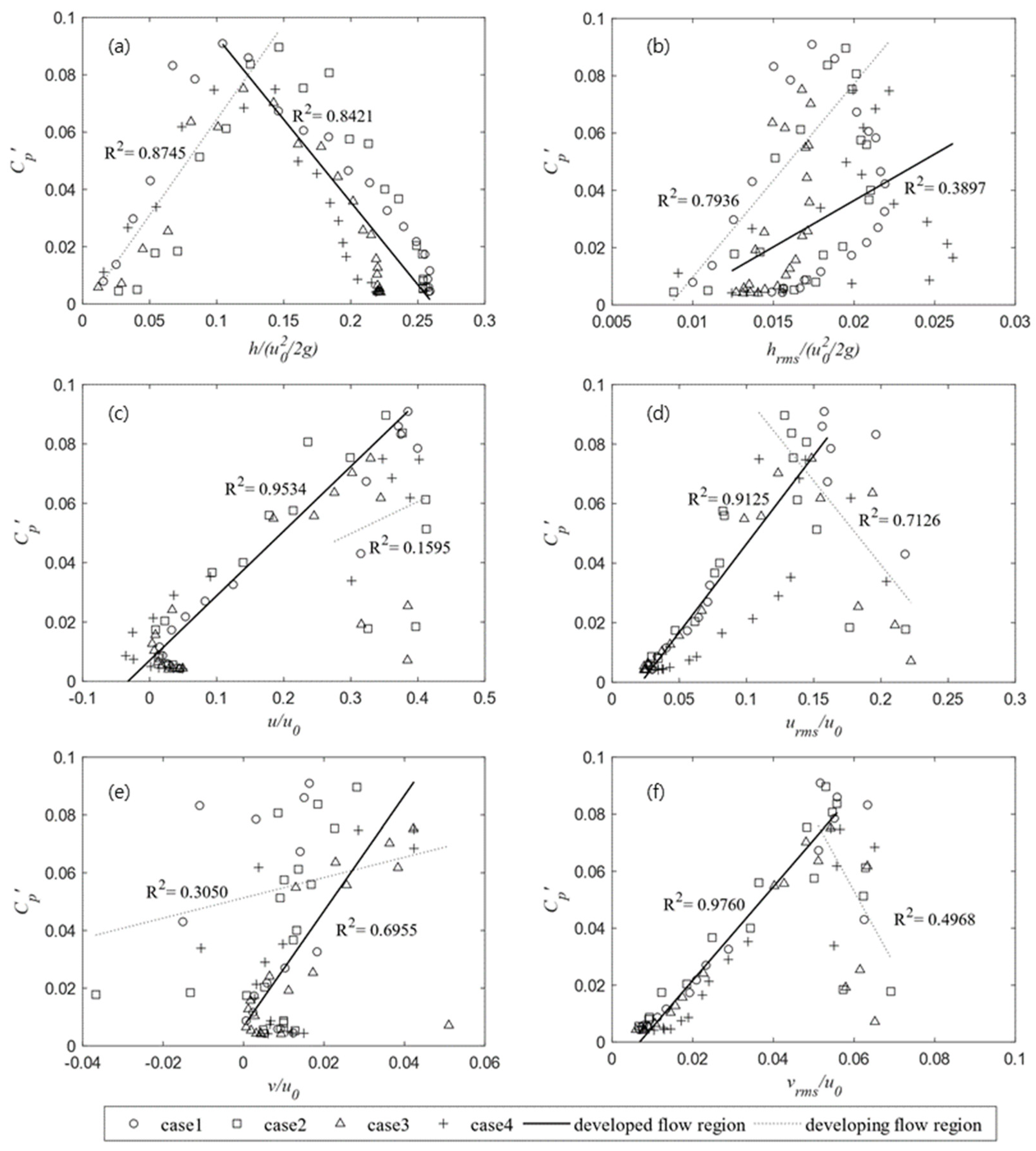
3.2. Analysis of Correlation between Flow Properties and Pressure Fluctuations

Correlation analysis was carried out to obtain relationships between the dimensionless variables of the flow property near the bottom (y = $y_o$) and the pressure fluctuation coefficients at the bottom in all conditions and at all measurement points. Six dimensionless variables were considered in this analysis: the water level, the water level fluctuation, the horizontal velocity, the horizontal turbulence intensity, the vertical velocity, and the vertical turbulence intensity. For this purpose, the velocities and the water levels from the same points where the pressure was measured were used. The characteristics of the incoming flows upstream of the hydraulic jump toe that were primarily used to normalize the variables in several previous studies were also used in this study. Figure 8 shows the correlations between the flow characteristics and the pressure fluctuation, which were conducted using the Pearson correlation coefficients given in

Table 2. Correlation coefficients of the dimensionless variables of the pressure fluctuations and the flow properties upstream and downstream of the locations of the pressure fluctuation peaks.

Flow Properties	$\mathit{h}/({\mathit{u}}_0^2/2\mathit{g})$	${\mathit{h}}_{\mathit{r}\mathit{m}\mathit{s}}/({\mathit{u}}_0^2/2\mathit{g})$	$\mathit{u}/{\mathit{u}}_0$	${\mathit{u}}_{\mathit{r}\mathit{m}\mathit{s}}/{\mathit{u}}_0$	$\mathit{v}/{\mathit{u}}_0$	${\mathit{v}}_{\mathit{r}\mathit{m}\mathit{s}}/{\mathit{u}}_0$
Entire section	−0.2980	0.3931	0.7904	0.6419	0.4063	0.7783
Developing air–water flow region	0.8745	0.7936	0.1595	−0.7126	0.3050	−0.4968
Developed air–water flow region	−0.8421	0.3897	0.9534	0.9125	0.6955	0.9760

.

In Figure 8, the different patterns are observed in the regions where the pressure fluctuation increases and decreases based on the point of the maximum pressure fluctuation. In the figure, the region of increased pressure indicates the developing air–water flow region (dotted line), i.e., $(x-x_1)/(y_0-H_u)\le 2 \mathrm{a}\mathrm{n}\mathrm{d} (x-x_1)/d1\le 20$, as previously mentioned by Chanson [31]. On the other hand, we refer to the pressure-reduced region as the developed air–water flow region (solid line in the figure). We assumed that the different patterns of these regions are due to the effect of the influencing factors depending on the regions. We analyzed the relationships in both the developing air–water flow region and the developed air–water flow region, respectively, in order to detect the differential effect of the factors.

The correlation coefficients are lower than 0.6 in the entire region and increase for all components when calculated separately. In particular, the dimensionless water level ($h/(u_0^2/2g)$) and the dimensionless turbulence intensity ($u_{rms}/u_0$, $v_{rms}/u_0$) are found to correspond to the pressure fluctuation coefficient ($C_p^{\prime }$). In Figure 8a, the coefficient reaches its maximum at the center of the stabilized water level. The correlations are obtained using the correlation coefficient of 0.8 or higher in both regions. This indicates that the water level is relevant to the pressure fluctuations in the developing air–water flow, showing that the increasing water levels are likely to provide the pressure fluctuations. After the midpoint as a transition point, the effect of the water level is not shown. Figure 8d,f show the relationships between the turbulence intensity and the pressure fluctuation coefficient, which show the similar patterns. In the developed air–water flow region, the relationships appear to be linear and show the high correlation coefficient of 0.9 or more. The dynamic pressure fluctuation is expected to play a more dominant role for the pressure fluctuation in the lower shear layer rather than the static pressure fluctuation, which significantly affects the pressure fluctuation in the upper shear layer [14].

In Figure 8b, the dimensionless water level fluctuation increases as the hydraulic jump begins. After the jump, it tends to converge to 0.012 due to the propagation of the surface wave downstream even without the roller. There is no clear relationship in the developed air–water flow region as indicated by the coefficient of 0.39. In Figure 8c,e, while the dimensionless horizontal velocity ($u/u_0$) and vertical velocity ($v/u_0$) have a relationship with the coefficients of 0.95 and 0.70, respectively, in the air–water developed region, there is no clear correlation for those in the developed air–water region. A limitation of this study is that in some cases the velocity measurements were not made in the impinging flow within the flow length of 10$y_0$. Since the air bubbles rarely reached this region, a part of the impinging flow was not measured, which might lead to the underestimation of the horizontal velocity. Although the horizontal velocity was underestimated, according to Lin et al. [20], the horizontal bubble velocity is equal to the horizontal water velocity near the bottom, so it is unlikely that the relationship is significantly different. In addition, the velocity and turbulence intensity appear to be larger in the initial part and the relationship with the pressure fluctuation is likely to be more obvious in the developing region.

The correlation analysis given in Figure 8 shows that the relationship between the turbulence intensity and the pressure fluctuation is most linearly correlated. Figure 9 also shows that the relationship between the horizontal and the vertical turbulence intensities is linear. The empirical equation between the two components of the turbulence intensity, Equation (7) was derived by combining Equations (5) and (6). The equation indicates that the horizontal turbulence intensity is larger than the vertical turbulence intensity of the local upstream wave speed of the weir by 0.03. In the equations, ${\rho }_w$ is the water density.

$$\frac{P_{rms}}{{\rho }_{w}g{H}_u}=\frac{u_{rms}}{\sqrt{g{H}_u}}-0.07$$

(5)

$$\frac{P_{rms}}{{\rho }_{w}g{H}_u}=\frac{v_{rms}}{\sqrt{g{H}_u}}-0.04$$

(6)

$$u_{rms}=v_{rms}+0.03\sqrt{g{H}_u}$$

(7)

Several previous studies have shown that the turbulence is related to the pressure fluctuations. In particular, Favre et al. [32] showed that Poisson’s equation can be used to demonstrate the relationship when the turbulent flow components are considered to be homogeneous and isotropic, as observed in Equation (8) [32,33]:

$$P_{rms}=\mathsf{\alpha }\mathsf{\rho }{\overline{u^{\prime }}}^2$$

(8)

where $\mathsf{\alpha }$ is the coefficient, $\rho$ is the density and $u^{\prime }$ represents the instantaneous velocity fluctuation. In order to define the magnitude of the pressure fluctuations, we used the turbulence intensity and the water level, which are very important factors in the correlation analysis. It was the first attempt to understand the mechanism of the bottom pressure fluctuations in the jump by comprehensively analyzing the flow properties and establishing their empirical relationship. The empirical equation with the correlation of $R^2=0.878$ based on the related variables is proposed as follows:

$$C_p^{\prime }=\alpha \exp \left[-{\left(\left(h^{*}/v^{*}-\beta \right)/\lambda \right)}^2\right]$$

(9)

where $h^{\mathrm{*}}(=h_{ave}/(u_0^2/2g\left)\right)$ is the dimensionless water level; $v^{\mathrm{*}}(=v_{rms}/u_0)$ is the dimensionless vertical turbulent intensity; and $\alpha$ = 0.1, $\beta$ = 0.407, and $\lambda$ = 1.215 are the empirical coefficients.

Equation (9) indicates that the magnitude of the pressure fluctuation depends on the ratio of the weight force and the turbulence intensity. Equation (9) is represented by the solid line in Figure 10. As shown in the figure, the pressure fluctuation increases rapidly as $h^{\mathrm{*}}/v^{\mathrm{*}}$ increases, reaches the maximum at $h^{\mathrm{*}}/v^{\mathrm{*}}$ = 1.5, and then decreases exponentially. It is observed that the maximum of the pressure fluctuation occurs at the point where the ratio of the dimensionless turbulence intensity to the dimensionless weight force is a constant. This suggests that the pressure fluctuations that depend on the turbulence intensity and the weight force may undergo a critical regime shift, thereby making the trends of the pressure fluctuations extremely different. With respect to the bubble transport, when $h^{\mathrm{*}}/v^{\mathrm{*}}$ is greater than or equal to 1.5, the effect of the natural convection is dominant due to the bubble rise caused by the buoyancy. On the other hand, if $h^{\mathrm{*}}/v^{\mathrm{*}}$ is less than 1.5, the effect of the turbulence intensity is dominant. In the turbulence-dominant region, the pressure fluctuations increase due to the increase in the weight force as the water level rises. Meanwhile, the natural convection-dominant region is not significantly affected by the impinging flow and thus the turbulence becomes weak.

4. Discussions

Many studies have focused on the fundamentals of the turbulent flows and the pressure fluctuations on the bottom in hydraulic jumps [5,9,10,11,12,13,14,20,32]. Most of these studies have provided a similar pattern of the pressure fluctuation that is relatively small near the toe, increases sharply in the roller region where the turbulence is amplified, and then decays exponentially downstream after the peak of the pressure fluctuation. Since the peak value is a key parameter for the design of riverbed protection structures such as stilling basins and aprons, the pressure fluctuation and its associated causes are of importance. Compared with the pressure fluctuation shown in Figure 6, the peak value of this study is relatively larger than that of the majority of other related studies [29,34]. This implies that the pressure fluctuation increases with the Froude number when the fluctuation is larger than the dynamic pressure, which corresponds to the results obtained by Hassanpour et al. [12]. In addition, it can be reasonably speculated that the higher pick results from the experimental conditions of lower Reynolds number in this study. According to Pinheiro [30], the maximum of the coefficients measured in a narrower channel with lower Reynolds number was larger than that in a wider channel. Specifically, de-aeration in the jump occurs more rapidly when the Reynolds number is low [35].

On the other hand, Nóbrega et al. [22] showed that both fluctuations of water level and pressure fluctuations have a similar behavior. That is, both fluctuations begin to increase at the toe, have a maximum value at the center of the roller, and then gradually decrease to a constant value. However, this showed a slight discrepancy with the results of this study. Based on the correlation analysis, it was shown that the correlation of the water level fluctuation is relatively insignificant, and the variation of the water level fluctuation is not clearly observed compared with the pressure fluctuation in the roller region (Figure 7). This is attributed to the difference in the Froude number. In the experiments of Nóbrega et al. [22], the Froude number was 2.98–5.26 and the Froude number of this study was 5.2–8.6, which is a relatively high. It implied that the water level fluctuation is not simply related to the pressure fluctuation acting on the bottom, but the pressure fluctuation can be varied via the complicated interaction between turbulent flows and free surface according to the flow conditions.

Through the comprehensive correlation analysis of the flow properties with the pressure fluctuation, the present results showed that the turbulence intensity and the water level are highly correlated with the pressure fluctuation. The dimensionless vertical turbulence intensity was related to the water level for the empirical relationship of the pressure fluctuation (Equation (9)). In the previous study [32], the pressure fluctuation was proportional to the square of the velocity fluctuation, while the results of the present study suggested a slightly different relationship. This may be because the hydraulic jump phenomenon causes a highly heterogeneous and anisotropic turbulent flow structure [1,36] contrary to the assumptions made by Lopardo [33] that the components are homogeneous and isotropic. In addition, the new dimensionless number, $h^{\mathrm{*}}/v^{\mathrm{*}}$, as the variable representing the effect of the buoyancy of the bubbly flow on the flow stability is suggested in Equation (9). $h^{\mathrm{*}}/v^{\mathrm{*}}$ is analogous to the Richardson number ($\mathrm{R}\mathrm{i}={gh/U}^2={Fr}^{-2})$, which denotes the ratio of forced convection and natural convection. Similarly, in the section adjacent to the toe of the hydraulic jump, the turbulence intensity is more dominant than the buoyancy due to the relatively high velocity and low water depth. We conclude that the pressure fluctuations in the jump are highly related to the convection of the bubbles. In other words, the pressure fluctuations result from the interaction of the influencing factors, such as the void fraction and the velocity fluctuation of the air–water flow in the hydraulic jump. The coefficients given in Equation (9) could be different due to several confined conditions related to scaling effects. It is necessary to examine these phenomena under various conditions, such as a wider range of Froude numbers and higher Reynolds numbers, in order to extrapolate to full scale applications.

5. Conclusions

When a hydraulic jump occurs in structures designed to protect a riverbed, such as stilling basins in spillways, the occurrence of pressure fluctuations can cause structural failure due to fatigue from repeated loading, the negative pressure to which concrete is vulnerable, and the maximum pressure that is higher than the regulated values specified in design standards. This study aimed to investigate the relationship between the flow properties in a hydraulic jump, thereby contributing to the further elucidation of the complex mechanism of pressure fluctuations caused by the hydraulic jump. Physical experiments were conducted under six conditions with different combinations of Froude number and jump toe position. Through these experiments, the instantaneous water level, velocity, and pressure were simultaneously measured, and the pressure fluctuation was coupled with the dimensionless variables of flow properties: specifically, water level, water level fluctuation, horizontal velocity, vertical velocity, horizontal turbulence intensity, and vertical turbulence intensity. The main results of this study are summarized as follows:

• The water level fluctuation had a minimal relationship with the pressure fluctuation at the bottom of the structure and the location of the maximum pressure fluctuation was identified at points where $(x-x_1)/(H_d-y_0)\approx$ 2.3.
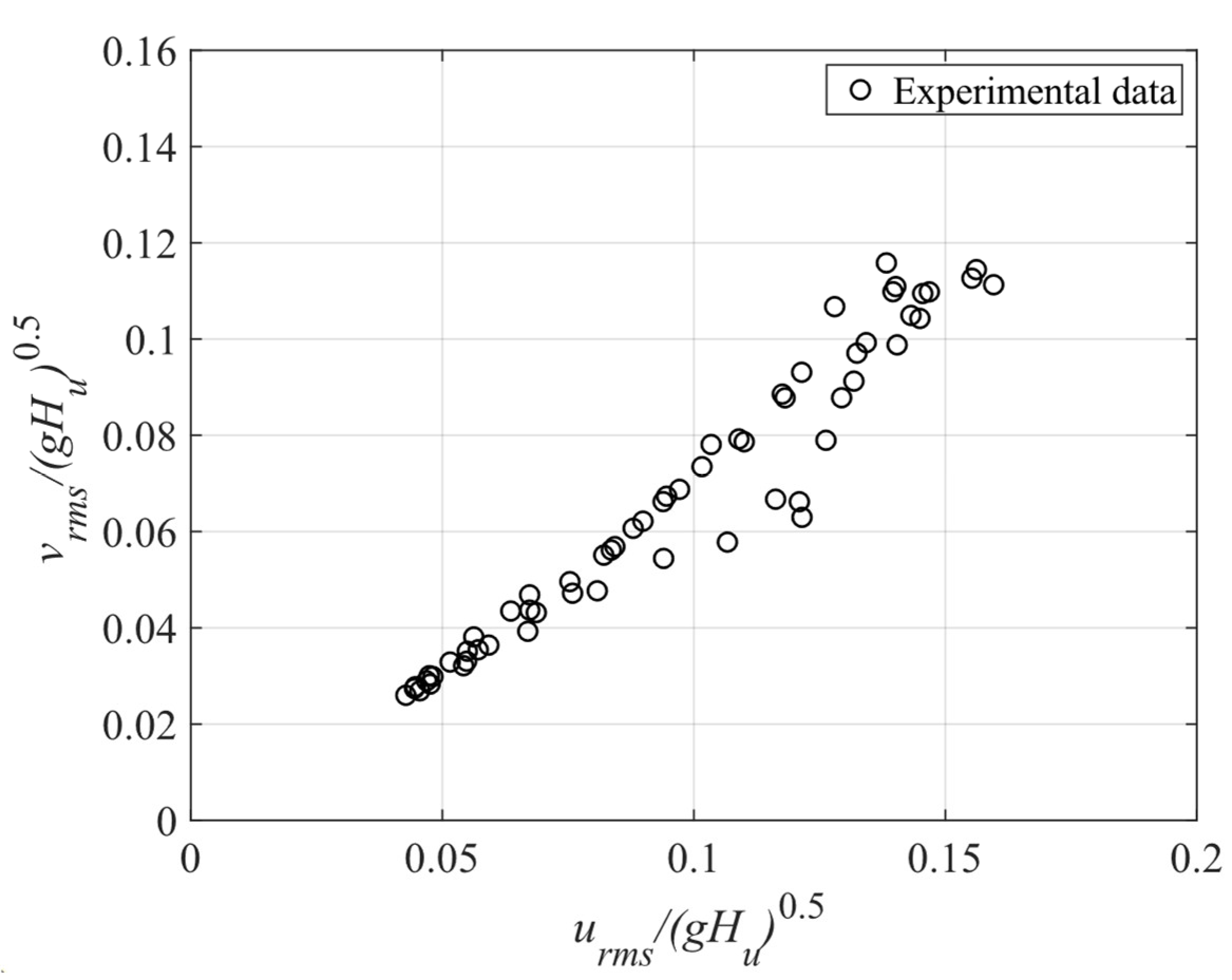
• A comprehensive correlation analysis between the flow properties and pressure fluctuations was performed by dividing the flow region into upstream and downstream areas from the maximum pressure fluctuation point. The analysis results indicated that the water level and turbulence intensity were the main factors influencing the pressure fluctuations. A linear relationship between the turbulence intensity and pressure fluctuation was demonstrated, and the horizontal turbulence intensity was consistently larger than the vertical one.
• An empirical formula was proposed for estimating the pressure fluctuation at the bottom of the structure using the novel dimensionless number. It was suggested that the pressure fluctuation under the influence of weight force and turbulence may undergo a critical regime shift and the trends of the pressure fluctuation may be significantly changed.

The turbulence intensity and water levels can be estimated, and the pressure exerted by the fluid on the structure can be predicted. Consequently, the pressure fluctuations in hydraulic jumps can be considered in the design of riverbed protection structures. Additionally, this result can help the designer to determine the location where reinforcement is required when installing the bed protection. It is expected that it can be used to derive improvement measures for the design and management of sustainable water structures.

In future research, it will be necessary to investigate the relationship between these variables under different experimental conditions with a wide range of Froude numbers. Since the void fraction was not investigated in this study, the effect of the void fraction needs to be analyzed.

References

1. Fiorotto, V.; Rinaldo, A. Fluctuating uplift and lining design in spillway stilling basins. J. Hydraul. Eng. 1992, 118, 578–596. [Google Scholar] [CrossRef]
2. Sobani, A. Pressure fluctuations on the slabs of stilling basins under hydraulic jump. In Proceedings of the 11th International Conference on Hydroinformatics, New York, NY, USA, 17–21 August 2014. [Google Scholar]
3. Kazemi, F.; Khodashenas, S.R.; Sarkarde, H. Experimental study of pressure fluctuation in stilling basins. Int. J. Civ. Eng. 2016, 14, 13–21. [Google Scholar] [CrossRef]
4. Narayanan, R. Cavitation induced by turbulence in stilling basin. J. Hydraul. Div. 1980, 106, 616–619. [Google Scholar] [CrossRef]
5. Wang, H.; Felder, S.; Chanson, H. An experimental study of turbulent two-phase flow in hydraulic jumps and application of a triple decomposition technique. Exp. Fluids 2014, 55, 1775. [Google Scholar] [CrossRef]
6. Zhao, Y.; Zhang, L.; Wang, W.; Tang, J.; Lin, H.; Wan, W. Transient pulse test and morphological analysis of single rock fractures. Int. Rock Mech. Min. Sci. 2017, 91, 139–154. [Google Scholar] [CrossRef]
7. Zhao, Y.; Wang, Y.; Wang, W.; Tang, L.; Liu, Q.; Cheng, G. Modeling of rheological fracture behavior of rock cracks subjected to hydraulic pressure and for field stresses. Theor. Appl. Fract. Mec. 2019, 101, 59–66. [Google Scholar] [CrossRef]
8. Graham, J.R.; Creegan, P.J.; Hamilton, W.S.; Hendrickson, J.; Kaden, R.A.; McDonald, J.E.; Noble, G.E.; Schrader, E.K. ACI 210R-93 Erosion of Concrete in Hydraulic Structures. ACI Mater. J. 1998, 93, 1–24. [Google Scholar]
9. Fiorotto, V.; Rinaldo, A. Turbulent pressure fluctuations under hydraulic jumps. J. Hydraul. Res. 1992, 30, 499–520. [Google Scholar] [CrossRef]
10. Toso, J.W.; Bowers, C.E. Extreme pressures in hydraulic jump stilling basins. J. Hydraul. Eng. 1988, 114, 829–843. [Google Scholar] [CrossRef]
11. Khader, M.H.A.; Elango, K. Repartition des pressions dans le domaine turbulent sous un ressaut hydraulique. J. Hydraul. Res. 1974, 12, 469–489. [Google Scholar] [CrossRef]
12. Hassanpour, N.; Dalir, A.H.; Bayon, A.; Abdollahpour, M. Pressure Fluctuations in the Spatial Hydraulic Jump in Stilling Basins with Different Expansion Ratio. Water 2021, 13, 60. [Google Scholar] [CrossRef]
13. Hasani, M.N.; Nekoufar, K.; Biklarian, M.; Jamshidi, M.; Pham, Q.B.; Anh, D.T. Investigating the Pressure Fluctuations of Hydraulic Jump in an Abrupt Expanding Stilling Basin with Roughened Bed. Water 2022, 15, 80. [Google Scholar] [CrossRef]
14. Wang, H.; Murzyn, F.; Chanson, H. Total pressure fluctuations and two-phase flow turbulence in hydraulic jumps. Exp. Fluids 2014, 55, 1847. [Google Scholar] [CrossRef]
15. Lennon, J.M.; Hill, D.F. Particle image velocity measurements of undular and hydraulic jumps. J. Hydraul. Eng. 2006, 132, 1283–1294. [Google Scholar] [CrossRef]
16. Liu, M.; Rajaratnam, N.; Zhu, D.Z. Turbulence Structure of Hydraulic Jumps of Low Froude Numbers. J. Hydraul. Eng. 2004, 130, 511–520. [Google Scholar] [CrossRef]
17. Montano, L.; Li, R.; Felder, S. Continuous measurements of time-varying free-surface profiles in aerated hydraulic jumps with a LIDAR. Exp. Therm. Fluid Sci. 2018, 93, 379–397. [Google Scholar] [CrossRef]
18. Ohtsu, I.; Yasuda, Y.; Gotoh, H. Hydraulic condition for undular-jump formations. J. Hydraul. Res. 2001, 39, 203–209. [Google Scholar] [CrossRef]
19. Si, J.-H.; Lim, S.-Y.; Wang, X.-K. Evolution of Flow Fields in a Developing Local Scour Hole Formed by a Submerged Wall Jet. J. Hydraul. Eng. 2020, 146, 4020040. [Google Scholar] [CrossRef]
20. Lin, C.; Hsieh, S.C.; Lin, I.J.; Chang, K.A.; Raikar, R.V. Flow property and self-similarity in steady hydraulic jumps. Exp. Fluids 2012, 53, 1591–1616. [Google Scholar] [CrossRef]
21. Ryu, Y.; Chang, K.-A.; Lim, H.-J. Use of bubble image velocimetry for measurement of plunging wave impinging on structure and associated greenwater. Meas. Sci. Technol. 2005, 16, 1945. [Google Scholar] [CrossRef]
22. Nóbrega, J.D.; Schulz, H.E.; Marques, M.G. Relation between free surface profiles and pressure profiles with respective fluctuations in hydraulic jumps. In Proceedings of the 4th IAHR Europe Congress, Liege, Belgium, 27–29 July 2016; pp. 629–636. [Google Scholar]
23. Nóbrega, J.D.; Schulz, H.E.; Zhu, D.Z. Free surface detection in hydraulic jumps through image analysis and ultrasonic sensor measurements. In Proceedings of the 11th National Conference on Hydraulics in Civil Engineering & 5th International Symposium on Hydraulic Structures, Brisbane, Australia, 25–27 June 2014; Engineers Australia: Sydney, Australia, 2014; p. 245. [Google Scholar]
24. Thielicke, W.; Stamhuis, E.J. PIVlab–Towards user-friendly, affordable and accurate digital particle image velocimetry in MATLAB. J. Open Res. Softw. 2014, 2, e30. [Google Scholar] [CrossRef]
25. Thielicke, W.; Stamhuis, E.J. PIVlab-Time-Resolved Digital Particle Image Velocimetry Tool for MATLAB; Online Resource; Figshare: London, UK, 2019. [Google Scholar] [CrossRef]
26. Wang, H.; Murzyn, F.; Chanson, H. Interaction between free-surface, two-phase flow and total pressure in hydraulic jump. Exp. Therm. Fluid Sci. 2015, 64, 30–41. [Google Scholar] [CrossRef]
27. Endres, L.A.M. Contribuição ao Desenvolvimento de um Sistema para Aquisição e Tratamento de Dados e Pressões Instantâneas em Laboratório. 1990. Available online: https://lume.ufrgs.br/handle/10183/195855 (accessed on 9 June 2023).
28. Lopardo, R.A. Internal flow of free hydraulic jump in stilling basins. In Proceedings of the 4th IAHR International Symposium on Hydraulic Structures, Porto, Portugal, 9–10 February 2012. [Google Scholar]
29. Marques, M.G.; Drapeau, J.; Verrette, J.-L. Flutuação de pressão em um ressalto hidráulico. Rev. Bras. Recur. Hídricos 1997, 2, 45. [Google Scholar]
30. Pinheiro, A.A.N. Acções Hidrodinâmicas em Soleiras de Bacia de Dissipação de Energia por Ressalto; Universidade Técnica de Lisboa: Lisbon, Portugal, 1995. [Google Scholar]
31. Chanson, H. Bubbly flow structure in hydraulic jump. Eur. J. Mech. B/Fluids. 2007, 26, 367–384. [Google Scholar] [CrossRef]
32. Favre, A.; Kovasznay, L.S.G.; Dumas, R.; Gaviglio, J.; Coantic, M. Turbulence in fluid mechanics: Theoretical and experimental foundations; statistical methods. NASA STI/Recon Tech. Rep. A 1976, 77, 22920. [Google Scholar]
33. Lopardo, R.A. Extreme velocity fluctuations below free hydraulic jumps. J. Eng. 2013, 2013, 678064. [Google Scholar] [CrossRef]
34. Murzyn, F.; Mouazé, D.; Chaplin, J.R. Air–water interface dynamic and free surface features in hydraulic jumps. J. Hydraul. Res. 2007, 45, 679–685. [Google Scholar] [CrossRef]
35. Chanson, H.; Gualtieri, C. Similitude and scale effects of air entrainment in hydraulic jumps. J. Hydraul. Res. 2008, 13, 35–44. [Google Scholar] [CrossRef]
36. Misra, S.K.; Kirby, J.T.; Brocchini, M.; Veron, F.; Thomas, M.; Kambhamettu, C. The mean and turbulent flow structure of a weak hydraulic jump. Phys. Fluids 2008, 20, 035106. [Google Scholar] [CrossRef]
Figure 1. Diagram of the experimental channel and the instrumental setup for the measurements: y 0 = the incoming supercritical flow before the jump; x 0 = the jump toe position; u 0 = the velocity of the incoming supercritical flow; H u = the water level upstream of the weir; and H d = the water level downstream of the hydraulic jump.
Sustainability 15 14246 g001
Figure 2. Example of the extracted water level points (orange circles).
Sustainability 15 14246 g002
Figure 3. Velocity fields for case 3 from the PIV and BIV measurements.
Sustainability 15 14246 g003
Figure 4. Comparison of the overlapping data between the PIV and BIV measurements in case 2: (a) the locations of the measurements; (b) the vertical profiles of the time-averaged velocity in the horizontal direction; (c) the vertical profiles of the time-averaged velocity in the vertical direction [20].
Sustainability 15 14246 g004
Figure 5. Flow characteristics of the hydraulic jump with Fr = 7.3: (a) the horizontal turbulence intensity; (b) the vertical turbulence intensity; (c) the horizontal velocity; (d) the vertical velocity.
Sustainability 15 14246 g005
Figure 6. Distribution of the pressure fluctuation coefficient along the hydraulic jump [22,27,28,29,30].
Sustainability 15 14246 g006
Figure 7. Longitudinal profiles of the depth-averaged flow properties in case 1: (a) the water level, (b) the pressure on the bottom.
Sustainability 15 14246 g007
Figure 8. Relationships between the dimensionless variables of the pressure fluctuations and the flow properties: (a) the water level; (b) the water level fluctuation; (c) the horizontal velocity; (d) the horizontal turbulence intensity; (e) the vertical velocity; (f) the vertical turbulence intensity.
Sustainability 15 14246 g008
Figure 9. Correlation between the horizontal and vertical turbulence intensities.
Sustainability 15 14246 g009
Figure 10. Dimensionless pressure fluctuations with the variations in the dimensionless water levels (h*) and the vertical turbulence intensities (v*).
Sustainability 15 14246 g010