Industrial Carbon Footprint (ICF) Calculation Approach Based on Bayesian Cross-Validation Improved Cyclic Stacking

Abstract

Achieving carbon neutrality is widely regarded as a key measure to mitigate climate change. The industrial carbon footprint (ICF) calculation, as a foundation to achieve carbon neutrality, primarily relies on roughly estimating direct carbon emissions based on information disclosed by industries. However, these estimates may not be comprehensive, timely, and accurate. This paper elaborates on the issue of ICF calculation, dividing a factory’s carbon emissions into carbon emissions directly produced by appliances and electricity consumption carbon emissions, to estimate the total carbon emissions of the factory. An appliance identification method is proposed based on a cyclic stacking method improved by Bayesian cross-validation, and an appliance state correction module SHMM (state-corrected hidden Markov model) is added to identify the state of the appliance and then to calculate the corresponding appliance carbon emissions. Electricity consumption carbon emissions come from the factory’s electricity consumption and the marginal carbon emission factor of the connected bus. Regarding the selection of artificial intelligence models and cross-validation technique required in the appliance identification method, this paper compares the effects of 7 cross-validation techniques, including stratified K-fold, K-fold, Monte Carlo, etc., on 14 machine learning algorithms such as AdaBoost, XGBoost, feed-forward network, etc., to determine the technique and algorithms required for the final appliance identification method. Experiment results show that the proposed appliance identification method estimates device carbon emissions with an error of less than 3%, which is significantly superior to other models, demonstrating that the proposed approach can achieve comprehensive and accurate ICF calculation.

1. Introduction

In recent years, greenhouse gas (GHG) emissions based on carbon dioxide have led to a global rise in temperature. This has become a common goal worldwide—mitigating climate change [1]. Global warming is now a severe challenge faced by the international community, mainly driven by excessive carbon dioxide emissions [2]. Energy consumption is causing escalating environmental pollution. Accurate carbon emission prediction is crucial for high-energy, high-emission enterprises to meet emission reduction targets [3]. Consequently, the international community has initiated measures to combat global warming, with a significant focus on carbon emissions accounting and prediction. These efforts are essential for developing and implementing emission reduction policies and calculating the “carbon emission tax” [4]. Therefore, the imperative to curtail carbon emissions presents a formidable and pressing challenge.

The precise quantification of carbon emissions is crucial for environmental goals, including combating global warming and achieving carbon equilibrium. This is essential for building a sustainable society and facilitating the transition to a low-carbon economy [5]. Considering the substantial impact of manufacturing on carbon emissions, accurately measuring carbon outputs associated with production facilities becomes critically essential. ICF calculation can obtain emission ratios, thereby clearly understanding the emission state of factories and providing a basis for emission reduction [6]. Currently, many research efforts focus on the industrial carbon emission calculation framework. However, most of these studies only consider direct carbon emissions during the industrial production process. They tend to overlook the carbon emissions resulting from electricity consumption. This omission leads to an incomplete understanding of the total emissions [7]. Furthermore, prevailing studies exhibit a generalized approach, deriving carbon emission estimates primarily from factories’ annual disclosures and other public data sources. Such broad temporal resolutions compromise precision, failing to satisfy the immediate and meticulous requirements for carbon emission curtailment [8].

Therefore, real-time ICF calculation is specifically important and worthwhile. This methodology bolsters the trustworthiness of carbon emission disclosure data, amplifying the societal accountability of manufacturing entities. Secondly, it enables immediate and precise surveillance of carbon discharges, optimizing the development and refinement of pertinent strategies for carbon emission mitigation [9]. Additionally, industrial carbon emissions constitute a significant portion of total carbon emissions. Therefore, precise ICF calculation is crucial. It offers a more precise and adaptable approach to forecasting carbon emissions. This capability is vital in addressing the ongoing environmental crisis. It forms the basis for achieving carbon neutrality, fostering sustainable social development, and mitigating the effects of climate change. Moreover, it provides valuable insights and references for global efforts to reduce carbon emissions.

A real-time ICF calculation approach is proposed, which facilitates precise and immediate quantification of industrial carbon emissions by examining the factory’s electricity data to discern the relevant device state. Within this framework, carbon emissions are bifurcated: device emissions originating from the manufacturing phase and electricity consumption emissions arising from electrical utilization. Pertaining to emissions from equipment, the functional state of the manufacturing apparatus is ascertained by examining the factory’s electricity data via appliance identification. Then, the device carbon emissions are calculated through the functional state of the device and the equivalent carbon emission capacity of the device. For electricity consumption carbon emissions, the electricity consumption for every projected time segment is determined based on the electricity data. Afterwards, the marginal carbon emission factor (MCEF) of the connected bus, to which the factory is interconnected with the power grid, is derived through the optimal power flow (OPF) [10]. Ultimately, emissions from electricity usage are determined using the calculated energy consumption and the marginal carbon emission factor.

In this study, the following technical advancements are introduced for the real-time industrial carbon emissions calculation.

(1)

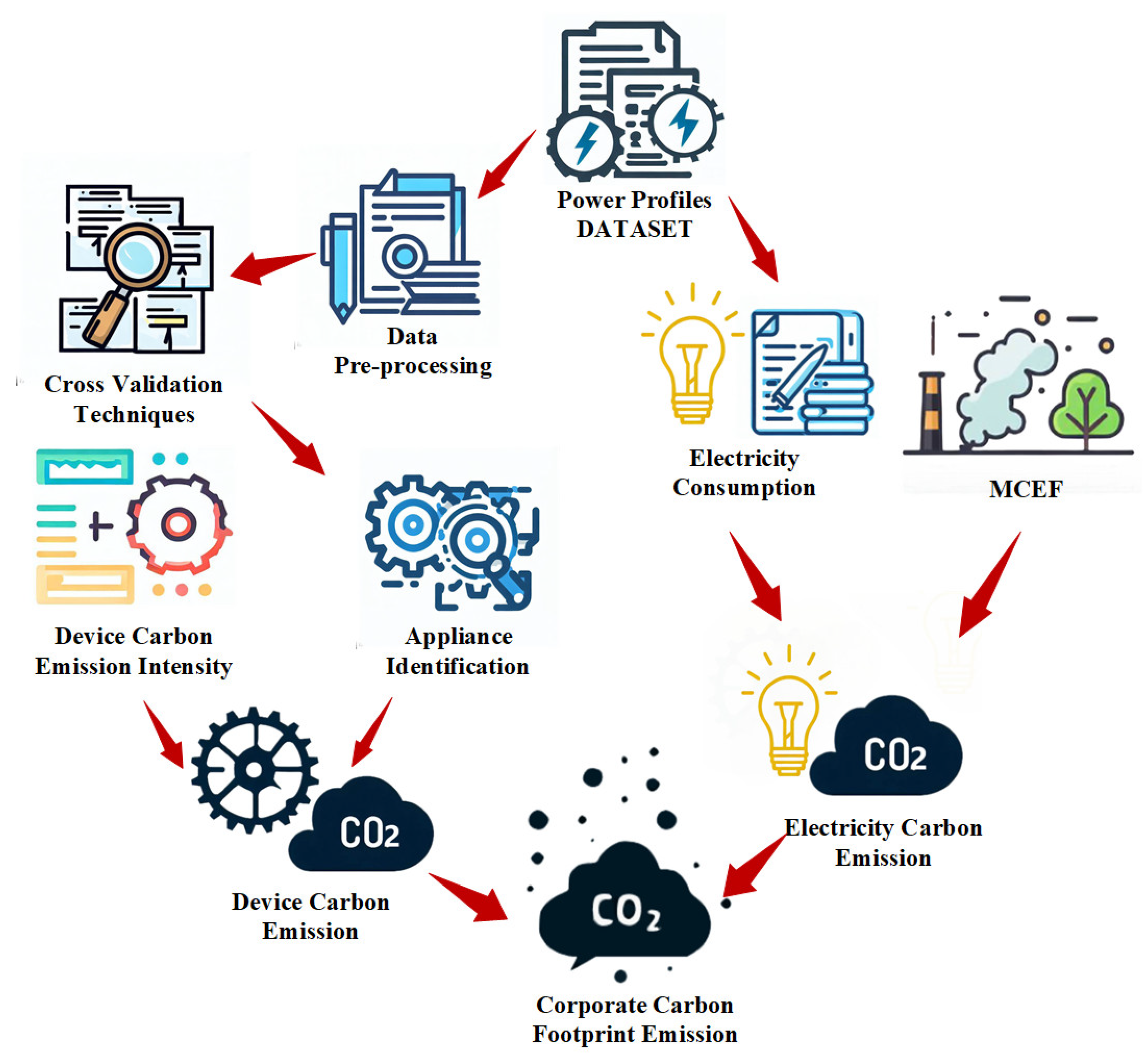
A real-time ICF calculation approach is proposed, which divides the carbon emissions of the factory into two categories. The appliance identification method and the technique for calculating MCEF based on DC-OPF are used, respectively, for calculation to obtain the total ICF calculation.

(2)

In response to the problem of real-time carbon emission calculation, an appliance identification approach based on Bayesian cross-validation improved cyclic stacking is proposed. This method can accurately monitor the state of the device and estimate the carbon emissions of the device with high precision. Moreover, based on the study of the characteristics of the operation state of industrial devices, a device state correction link SHMM is proposed to correct the appliance identification results.

(3)

A total of 7 cross-validation techniques and 14 machine learning models are compared to determine the artificial intelligence models and cross-validation technique required for the appliance identification model.

The rest of this paper is organized as follows. Section 2 introduces the related work. The theory and method are seen in Section 3. The details of ICF distribution calculation are discussed in Section 4. Section 5 introduces the experiment and results. Finally, Section 6 summarizes this paper.

2. Related Works

2.1. ICF Calculation

As concerns over climate change intensify and the urgent need to maintain the global temperature increase below 1.5 °C becomes increasingly apparent, carbon emissions have drawn significant attention from scholars and policymakers. Carbon accounting, which is crucial for carbon management and mitigation, involves a range of tasks related to carbon emissions, including quantification, calculation, validation, and documentation [11].

While the carbon footprint, a key component of carbon accounting, lacks a standardized definition, it has been proposed and widely adopted across various sectors of society. Generally speaking, CF is conceptualized as the quantification of total CO₂ emissions, both direct and indirect, attributable to a specific entity [12]. Such an “entity” encompasses processes, products, individuals, organizations, corporations, governmental bodies, and more. Quantifying ICF offers advantages to businesses and the broader society, including furnishing data for carbon disclosure and facilitating a shift towards sustainable practices, among others [13]. This study primarily delves into CO₂ emission quantification at the organizational level.

To address the limitations of existing methods, several studies have utilized various models and algorithms to estimate the carbon emissions produced by different types of entities. Some studies have evaluated regional carbon footprints by establishing statistical and machine learning models. Ref. [14] has built a Bi-LSTM-based emission prediction model to forecast the carbon emissions in the South Asian region. Based on an improved particle swarm optimization algorithm, Ref. [15] proposes an improved Gaussian process regression method for predicting carbon emissions in a certain province of China. Some teams have conducted research on the disclosure of corporate carbon emissions. Refs. [9,10] uses a two-step framework, combining predictions from multiple base learners using a meta-elastic network learner, to predict corporate carbon emissions for investor risk analysis. There are also some studies in the literature that have studied the problem of carbon emission calculation in certain industrial production processes. Ref. [16] monitors carbon dioxide emissions based on the electrical energy used and coal burned during the production process, and establishes a support vector machine model to estimate carbon emissions in the alcohol industry. Ref. [17] discusses the performance of three machine learning algorithms (ANN, SVM, and DL) in predicting greenhouse gas emissions in power production. Ref. [18] proposes an innovative model based on deep neural networks for estimating tank-to-wheel carbon dioxide emissions utilizing the dynamic programming (DP) approach. Ref. [19] proposes an integrated deep learning model for exhaust emission prediction, integrating four prediction engines, namely ANN, ELM, SVM, and LSSVM, to achieve initial emission prediction. Ref. [20] uses a large amount of real-world data collected from established steel plant smelting workshops, and establishes an energy value prediction model for electric arc furnaces (EAFs) through data-driven methods to estimate the carbon emissions of electric arc furnaces. In terms of the scope of research, the majority of the research in this domain is tailored specifically for either individual production processes or industries, and some are studies of regional carbon footprints, which are not entirely applicable to other industries. In terms of research methods, many teams estimate carbon footprints by establishing statistical models and machine learning models. The algorithms employed are relatively traditional and simplistic. Furthermore, some integrated models proposed in the literature do not fully leverage the strengths of each individual model to enhance predictive performance. Therefore, an ICF calculation approach based on appliance identification is proposed.

2.2. Nonintrusive Load Monitoring

Appliance load monitoring (ALM) aims to offer granular device state detection and furnish segmented energy consumption insights. Predominantly, there exist two ALM methodologies: intrusive load monitoring (ILM) and nonintrusive load monitoring (NILM) [21]. While ILM necessitates the placement of a meter between every observed device and its corresponding socket, NILM mandates a singular meter at the ingress point. Consequently, due to its reduced installation and upkeep expenses, NILM emerges as a more feasible approach [22].

NILM, often referred to as load disaggregation, endeavors to discern the operational state (on/off) and exact electricity utilization of distinct electrical loads, utilizing solely their cumulative consumption as input. Implicit in its “nonintrusive” designation, this technique is executed with limited intrusion into user confidentiality [23]. Data acquisition is centralized to a singular point (aggregate load), obviating the necessity for supplementary device installations, thereby mitigating both intricacy and expenditure [24].

The NILM of household appliances has several identification methods and applications. These methods can be mainly divided into two categories: traditional methods based on machine learning and methods based on deep learning. For traditional methods based on machine learning, in [25], the authors used several multilayer perceptions with varied hyperparameter configurations for load discernment. Subsequent analyses revealed that distinct devices exhibited optimal performance under specific hyperparameter combinations. Using the transient signals in the system, a household appliance monitoring method based on decision trees was designed [26]. Predominantly, these techniques necessitate data of elevated sampling rates, mandating the use of high-frequency instrumentation for data acquisition. However, constrained by the learning capacities of the adopted models, they grapple with extensive datasets exhibiting intricate appliance traits. Conversely, leveraging the robust feature extraction process of deep neural networks, deep learning has garnered notable accomplishments in domains like computer vision, speech recognition, and natural language processing. The integration of deep-learning-centric approaches in NILM within residential settings has garnered academic attention. In [27], a feed-forward neural network (FFNN) was proposed to extract the electricity consumption signals of three appliances. Ref. [28] introduced a convolutional variational autoencoder tailored for isolating device-specific signals from the primary device. This model, benchmarked on the UK-DALE dataset, showcased leading-edge performance. A similar variational autoencoder for NILM was delineated in [29], where a variational recurrent neural network (VRNN) was employed to craft device signals, utilizing total electricity consumption as an input. In the study presented in [30], a tri-component network was proposed: the seed source S, analogous to the encoder segment in the DAE model; G, tasked with crafting new signal waveforms from the DAE’s latent space; and D, a binary classifier designed to discern genuine from fabricated signals. A subsequent enhancement to this framework was articulated in [31], where the authors integrated two gated recurrent units into the D network for enhanced discrimination. Pan et al. [32] deployed a cGAN for energy disaggregation, with the G component being a 1-D UNet, processing the main signal to produce device-specific signals, while D comprised a convolution-centric architecture with multiple layers. This approach adopted a sequence-to-subsequence output, selecting the optimal output window based on the estimation timeframe during training. Finally, GAN-NILM was proposed in [33]. The network consists of an autoencoder G, responsible for generating device-specific signals. The researchers linked the power signal to G’s output, positing that this approach enhances training stability. The discriminator’s objective is to discern the authenticity of the decomposed signal. Furthermore, the second-to-last layer of D produces output features, which are subsequently supplied to G in the ensuing iteration. Employing a consistent parameter-sharing technique, they modeled a transferable generative framework and evaluated it across three open-access datasets. However, existing research data on low-frequency ALM predominantly focus on residential consumers or are confined to a singular industrial sector.

The composite power sequence is characterized as a temporal array, in which data points encompass not only contextual details but also display differential correlations across the temporal spectrum. It is conventionally observed that data points closer in time exhibit enhanced correlation. Prevailing studies harness techniques rooted in neural networks or recurrent neural networks (RNNs) to derive contextual insights from the entire sequence, neglecting pivotal data intrinsically linked to the objective. Such methodologies remain deficient in discerning the temporal interdependencies present in electricity data, thereby undermining the precision of ALM for industrial stakeholders. Moreover, while residential entities typically demonstrate invariant behavioral attributes and consumption modalities, industrial consumption is predominantly molded by sectoral nuances, operational agendas, and the presence or absence of shift-based operations [34]. Hence, the demands of industrial NILM exceed those of residential contexts, introducing augmented complexities. This situation necessitates the development of an innovative approach skilled at meticulously separating both contextual and significant temporal data, thereby enhancing the effectiveness of appliance identification.

3. Materials and Methods

3.1. ICF Calculation Approach Statement

A real-time ICF calculation approach is proposed, which facilitates precise and immediate quantification of industrial carbon emissions by examining the factory’s electricity data to discern the relevant device state. Within this framework, carbon emissions are bifurcated: device emissions originating from the manufacturing phase and electricity consumption emissions arising from electrical utilization. Pertaining to emissions from equipment, the functional state of the manufacturing apparatus is ascertained by examining the factory’s electricity data via appliance identification. Then, the device carbon emissions are calculated through the functional state of the device and the equivalent carbon emission capacity of the device. For electricity consumption carbon emissions, the electricity consumption for every projected time segment is determined based on the electricity data. Afterwards, the MCEF of the connected bus, to which the factory is interconnected with the power grid is derived through the OPF. Ultimately, emissions from electricity usage are determined using the calculated electricity consumption and the marginal carbon emission factor. The methodology for real-time ICF calculation is shown in Figure 1.

The real-time ICF calculation facilitates the immediate quantification of carbon emissions from various manufacturing entities. A certain factory CF in the period $T_p$ with an estimated interval of $\mathit{\tau }$ is divided into device emissions and electricity emissions. The component of device emissions pertains to the direct release from the device throughout the manufacturing phase, while the electricity emissions represent the secondary discharges associated with the energy utilization of the generator in the electricity utilization stage of the device. Therefore, for a factory with $\mathit{\varpi }$ device $De=\{d_1,d_2,\dots ,d_{\varpi }\}$, the cumulative CF $E_t$ can be denoted by $E_t=E_d+E_i$, where $E_d$ is the device CF, and $E_i$ is the electricity CF due to the use of electricity. Equation (1) can be used to estimate $E_d$.

$$E_d={\displaystyle \sum _{j=1}^{\tau }{\displaystyle \sum _{i=1}^{\varpi }{\lambda }_{S_{i,j}}\times \frac{T_p}{\tau }}}$$

(1)

where ${\lambda }_{S_{i,j}}$ delineates the carbon emission capacity of device $i$ in the time span $j$, and $S_{i,j}$ characterizes the operational state of device $i$ during span $j$. $E_i$ is obtained by using Equation (2).

$$E_i={\displaystyle \sum _{j=1}^{\tau }{\xi }_j\times U_j\times \frac{T_p}{\tau }}$$

(2)

where ${\xi }_j$ is the MCEF of the connected bus to which the manufacturing entity is interconnected, and $U_j$ is the electricity usage.

The accurate CF calculation hinges on obtaining the device state $S$, the equivalent carbon emission capacity of the device $\lambda$, the MCEF $\xi$, and the electricity consumption $U$. Typically, a factory’s device has its fixed state, and factories of the same type have similar devices. Thus, the $S$ is identified via appliance identification. The carbon emission capacity of the device $\lambda$ can be collected with relative ease. The MCEF $\xi$ can be calculated through the OPF, and the electricity usage $U$ can be directly obtained from the smart meter.

The details of the real-time ICF calculation process are as follows, with some theories introduced in subsequent chapters. Firstly, electricity data are harnessed as foundational input for both appliance identification and electricity usage. By utilizing the proposed appliance identification technique, the $S$ can be identified. Combined with the carbon emission capacity $\lambda$, the $E_d$ of the device can be calculated. For the $E_i$ caused by electricity use, within a predefined power system architecture, the generator dispatching schedule is derived through the resolution of the OPF. Combined with the corresponding generator carbon emission factor, the generator carbon emission $E_G$ is derived. Subsequently, by adding a singular element to the bus capacity where the manufacturing facility is located, and reengaging the OPF, a new dispatching schedule is obtained. Utilizing this revised dispatching schedule and the associated generator factor, the new carbon emission amount $E_G^{\prime }$ is calculated. Next, the following formula can be used to calculate the MCEF $\xi$ of the connected bus.

$$\xi =E_G{}^{\prime }-E_G$$

(3)

The electricity consumption can be directly derivable from the power data. The carbon emissions from electricity consumption can be obtained via Equation (2). Finally, $E_t$ are the sum of $E_d$ and $E_i$.

3.2. Appliance Identification Technology

Through data acquisition from a singular meter positioned at the ingress point, NILM is adept at discerning the operational state of devices. This paper proposes an appliance identification method based on Bayesian cross-validation improved cyclic stacking. This method optimizes the hyperparameter set of multiple models integrated by stacking based on the combination of Bayesian and cross-validation. It improves the stacking model structure by cyclically applying meta-models and base models. The architecture is shown in Figure 2.

The approach encompasses four integral components: data embedding, relationship learning, state recognition, and state correction. This methodology harnesses the total power sequence from the factory as its foundational input. Within the first part, the initial power sequence $X$ undergoes transformation into $\overline{X}$, characterized by integral values, as delineated through Equation (4), wherein $\min (X)$ represents the minimal value within $X$. Subsequently, $\overline{X}$ is segmented into an array of power subsequences denoted as $\tilde{X}$, each with a length of $L$.

$$\overline{X}=\left[\frac{X}{\min (X)}\right]$$

(4)

After that, the input is derived from the embedding matrix. This vector sequence of the embedding matrix is divided into n equal-length subsequences according to the number of base models. First, for each type of base model, the cross-validation technique is used to evaluate the impact of these hyperparameters on model performance based on the hyperparameter set selected at the initial time [35]. Each subsequence is divided according to a certain rule, with one part selected as the validation set and the rest as the training set. Then, for the initial hyperparameters, the base model is trained with this training set, and the model performance is evaluated with the validation set. The objective function used to measure model performance is the negative value of the F1 score. For each group of hyperparameters $\theta$, the objective function can be represented by Equation (5), and each objective function is composed of Equations (6) and (7).

$$f(\theta )=-F1(\theta )=-2\cdot \frac{\mathrm{Precision}\cdot \mathrm{Recall}}{\mathrm{Precision}+\mathrm{Recall}}$$

(5)

$$\mathrm{Precision}=\frac{\mathrm{TP}}{\mathrm{TP}+\mathrm{FP}}$$

(6)

$$\mathrm{Recall}=\frac{\mathrm{TP}}{\mathrm{TP}+\mathrm{FN}}$$

(7)

where TP (true positive) denotes the count of samples correctly classified by the model as positive cases. FP (false positive) represents the tally of samples erroneously classified by the model as positive cases. FN (false negative) signifies the quantity of samples inaccurately classified by the model as negative cases.

This process is repeated for all divided vector sequences, and we obtain the average performance indicator of the base model under the action of this group of hyperparameters. Next, the above process is repeated for the remaining initial hyperparameter groups, and the average performance indicator of the base model corresponding to each group of hyperparameters is obtained.

Then, based on the initial hyperparameter combination and the corresponding average performance indicator, a Bayesian optimization model is established [36]. The Gaussian process (8) is chosen as the prior distribution, and Expected Improvement (9) is chosen as the acquisition function.

$$p(f|\theta ,D)=\frac{p(D|f,\theta )p(f|\theta )}{p(D|\theta )}$$

(8)

$$EI(\theta )=\left\{\begin{array}{ll}(\mu -f_{min}+v)\mathrm{\Phi }(Z)+\sigma \varphi (Z),\hfill & \mathrm{if} \sigma >0\hfill \\ 0,\hfill & \mathrm{if} \sigma =0\hfill \end{array}\right.$$

(9)

where $D$ represents the known set of hyperparameters and their corresponding F1 score, $f$ is the prediction of the F1 score, and $p(f|\theta ,D)$ is the posterior probability. $\mu$ and $\sigma$, respectively, represent the expected value and standard deviation; $f_{min}$ is the smallest value observed so far; and $v$ is an adjustment parameter used to balance exploration and exploitation, where $\mathrm{\Phi }$ and $\varphi$ are, respectively, the cumulative distribution function and probability density function of the standard normal distribution.

Under the Bayesian optimization framework, the objective function is considered a stochastic function of the hyperparameters, and its prior distribution is a Gaussian process. Subsequently, through an iterative process, new combinations of hyperparameters are continuously sought. In each iteration, the expected improvement (EI) value of all possible hyperparameter combinations is calculated, and the combination with the largest EI value is selected as the hyperparameter combination for the next evaluation.

Subsequently, the new hyperparameter combination is fed back to the base model, which uses the new hyperparameter combination for cross-validation to obtain its average performance indicator F1 score. Then, the Bayesian optimization model is updated using the new hyperparameter combination and its average performance indicator.

This iterative process continues until the preset stop condition is met, i.e., the gain of the EI value is less than the preset threshold after five consecutive iterations. At the end of the entire iterative process, the combination with the best average performance F1 score among all explored hyperparameter combinations is selected as the optimal hyperparameter combination. Finally, each base model selects the optimal hyperparameter combination to predict the subsequence, and employs Softmax as the activation mechanism to derive the associated likelihood of the device existing in varied modes given a specific load sequence. Ultimately, the state with a probability surpassing a predefined threshold is designated as the device’s operational state, culminating in the formation of the device state subset pertinent to each foundational model. The n device state subsets are combined to form the input sequence of the meta-model. The Bayesian cross-validation optimization model is used to optimize the meta-model, predict the input sequence, and form the total device operating state set.

In terms of the stacking structure, this paper proposes a new type of cyclic stacking architecture, which alternately uses six different machine learning models as meta-models, and the remaining models are used as base models, forming six different model structures. In this way, not only is the performance of each model fully evaluated, but also their performance differences when they are used as meta-models and base models are compared. Finally, by selecting the model structure with the best performance, the optimal prediction result is obtained, thereby obtaining the device state set predicted by the Bayesian cross-validation improved cyclic stacking model.

In addition, in the data post-processing part, a SHMM, which is a state correction module composed of a hidden Markov model [37], is proposed, which uses the state transition probability and observation probability of the state correction module to adjust these prediction results to make them more in line with the actual operating state of the device. If the operating state of the device usually remains unchanged for a period of time and does not mutate, then the state transition probability of this state correction module will be very high, which means that the device is more likely to stay in the same state. Therefore, if a state mutation appears in the prediction result, the state correction module may consider this mutation as unreasonable and correct this prediction result. The obtained device state set is input into the state correction module to monitor and correct abnormal state values in the process of device operation state, in order to improve the final ICF calculation accuracy.

For a state set $S=\{s_1,s_2,\dots ,s_n\}$ and observation set $Y=\{y_1,y_2,\dots ,y_m\}$, the SHMM has:

$$A=[a_{ij}]=[P(q_{t+1}=s_j|q_t=s_i)]$$

(10)

$$B=[b_{ij}]=[P(o_t=y_j|q_t=s_i)]$$

(11)

$$\pi =[{\pi }_i]=[P(q_1=s_i)]$$

(12)

Here, $P(q_{t+1}=s_j|q_t=s_i)$ represents the probability of transitioning to state $s_j$ at time $t$+1 given that it is in state $s_i$ at time $t$. Here, $q_t$ represents the hidden state at time $t$. $b_{ij}$ represents the probability of observing $y_j$ given that it is in state $s_i$ at time $t$. Here, $o_t$ represents the observed state at time $t$. ${\pi }_i$ represents the probability of being in state $s_i$ initially. In the process of correcting predictions with the hidden Markov model, the Viterbi algorithm is commonly used to find the most likely hidden state sequence. Firstly, the model is initialized, and for each state $i$, the probability of being in state $s_i$ initially and observing $o_1$ is calculated:

$${\delta }_{t=1}(s_i)={\pi }_i\times b_i(o_1)$$

(13)

$${\psi }_{t=1}(s_i)=0$$

(14)

where ${\delta }_{t=1}$ represents the probability of being in state $s_i$ at time $t$ = 1 and the probability of generating observation o from state $s_i$. ${\pi }_i$ is the initial state probability, indicating the probability of being in state $s_i$ at the start. $b_i(o_1)$ is the observation probability, indicating the probability of generating observation $o_1$ in state $s_i$.

${\psi }_{t=1}$ represents the index of the most likely previous state when in state $s_i$ at time $t$ = 1. Since we do not have a previous state at time $t$ = 1, ${\psi }_{t=1}(s_i)$ is initialized to 0. Then, the state probability is recursively calculated. For each time $t=2,3,\dots ,T$ and each state $s_i$, find the probability of the most likely state sequence at time $t$ in state $s_i$ and the last state $s_j$ of this sequence:

$${\delta }_t(s_i)={\max }_{s_1\le s_i\le s_n}[{\delta }_{t-1}(s_j)·a_{ji}]·b_i(o_t)$$

(15)

$${\psi }_t(s_i)=\arg {\max }_{s_1\le s_j\le s_n}[{\delta }_{t-1}(s_j)·a_{ji}]$$

(16)

Here, ${\delta }_t(s_i)$ represents the probability of the most likely state sequence ending at time $t$ with the last state being $s_i$. This probability is obtained by multiplying the maximum probability ${\delta }_{t-1}(s_j)$ of all possible states at the previous time, the probability $a_{ji}$ of transitioning from state $s_j$ to state $s_i$, and the probability $b_i(o_t)$ of generating observation $o_t$ in state $s_i$.

${\psi }_t(s_i)$ represents the index of the most likely previous state at time $t$ in state $s_i$. This index is obtained by multiplying the maximum value of the maximum probability ${\delta }_{t-1}(s_j)$ of all possible states at the previous time and the probability $a_{ji}$ of transitioning from state $s_j$ to state $s_i$.

Next, find the probability and state of the optimal path at time T.

$$P^{\ast }={\max }_{s_1\le s_i\le s_n} {\delta }_T(s_i)$$

(17)

$$q_T^{*}=\arg {\max }_{s_1\le s_i\le s_n} {\delta }_T(s_i)$$

(18)

where $P^{\ast }$ represents the probability of the most likely state sequence, which is obtained from the maximum probability ${\delta }_T(s_i)$ of all possible states at the last time. $q_T^{*}$ represents the last state of the most likely state sequence, which is obtained from the maximum probability ${\delta }_T(s_i)$ of all possible states at the last time corresponding to the value of $s_i$.

Finally, perform backtracking. For each time $t=T-1,T-2,\dots ,1$, backtrack to find other states of the optimal path:

$$q_t^{*}={\psi }_{t+1}(q_{t+1}^{*})$$

(19)

where $q_t^{*}$ represents the t-th state of the most likely state sequence, which is obtained from the index ${\psi }_{t+1}(q_{t+1}^{*})$ of the most likely previous state corresponding to the most likely state $q_{t+1}^{*}$ at the next time.

In this way, we can start from the last time and backtrack to get all states, thus obtaining the most likely state sequence. So far, we have obtained the most likely hidden state sequence $q^{*}=q_1,q_2,\dots ,q_T^{*}$.

Align the obtained state sequence according to time $t$, compare the device state predicted by the Bayesian cross-validation improved cyclic stacking model and the device state corrected by the state correction module, detect the time point of state mutation, and use the corrected state of the state correction module to replace the mutated state.

3.3. Algorithm Selection

In the “structure of the proposed appliance identification approach”, it is necessary to determine the cross-validation technique and the artificial intelligence algorithms required for the ensemble model. This paper adopts an algorithm selection method based on experimental feedback effects. It applies seven cross-validation techniques: stratified K-fold, K-fold, Monte Carlo, hold-out, leave-p-out, leave-one-out, and repeated K-fold. The classification model is enhanced with fourteen artificial intelligence algorithms: AdaBoost, XGBoost, feed-forward network, KNN, random forest, multilayer perceptron, support vector classifier, decision tree, gradient boosting, Gaussian processes, naïve Bayes, extreme learning machine, CNN, and LightGBM. The effects of these algorithms are compared after optimization to determine the artificial intelligence models and cross-validation technique required for the appliance identification model.

Table A1. Descriptions of cross-validation techniques.

Models	Description
K-Fold	A dataset is divided into k subsets, and the learned model is then tested on the remaining subsets. Each of the “k” subsamples is utilized precisely once as validation data after the cross-validation technique has been applied k times. The k estimates may then be averaged [60].
Leave-P-Out	Cross-validation uses P samples from the sample set as the test set and the remainder of the samples as the training set. It requires n area samples, and takes $C_n^p$ times to train and test the model. The sample set is denoted by S. This is carried out again until the original sample is clipped on the training dataset and the validation data of p observations [61].
Leave-One-Out	In leave-p-out cross-validation, the value of P is set to one.
Hold-Out	Data points are randomly assigned to the training set and the test set. Each set’s size is arbitrary, but often, the test set is smaller than the training set. After that, the set is tested on test data and then trained using test data [62].
Repeated K-Fold	All that is needed is to repeatedly execute the Cross-Validation approach and provide the mean outcome across all folds from all runs. A high number of calculations is always desired to provide trustworthy performance calculation or comparison [60].
Stratified K-Fold	Stratified folds are produced by the cross-validation class, a K-fold variation. The folds are produced by maintaining a consistent proportion of observations for each class. This ensures that each dataset fold has the same percentage of instances with each label. When seeking to make inferences from multiple sub-groups or strata, stratified sampling is a typical sampling strategy [63].
Monte Carlo	The dataset is randomly split into training and validation data using Monte Carlo cross-validation. The model is fitted to the training instances for each such split, and the anticipated accuracy is determined using the validation data. The outcomes of the splits are then averaged [64].

is an introduction to 7 cross-validation techniques. Table A1 is provided in the Appendix A.

3.3.1. LightGBM

LightGBM is a machine learning framework based on the gradient-boosting decision tree algorithm. It is characterized by its efficiency, speed, and high accuracy, making it particularly suitable for handling large-scale data [38].

LightGBM employs a two-fold approach in constructing the framework. The first method, gradient-based one-side sampling, prioritizes random sampling for gradient computation. The second technique, exclusive feature bundling, groups specific features together to effectively reduce feature dimensionality. This concerted effort is geared towards diminishing feature dimensionality and subsequently enhancing prediction accuracy by significantly reducing sample processing time [39].

In the context of a given supervised training dataset, the objective of LightGBM is to identify an approximation function. This function aims to minimize the expected value of the designated loss function. The specific loss function formula is shown in Equation (20)

$$F_M(x)={\displaystyle \sum _{m=1}^M{\gamma }_m}{h}_m(x)$$

(20)

where ${\gamma }_m=argmin{\displaystyle {\sum }_{i=1}^{n}L(y_i,F_{m-1}(x_i)+\gamma h_m(x_i)})$, M is the maximum number of iterations, and $h_m(i)$ is the basic decision tree.

3.3.2. XGBoost

Following the concept of gradient boosting, XGBoost typically adopts a decision tree as its foundational classifier. It incrementally constructs a composite model of multiple decision trees using a greedy algorithm, aiming to minimize the associated cost [40]. Therefore, the XGBoost model can be expressed as:

$${\widehat{y}}_t={\displaystyle \sum _{m=1}^M{f}_m(x_i)}$$

(21)

Type: ${\widehat{y}}_t$ is the samples in the $x_i$ forecast, $M$ is the number of trees, and $f_m$ is the m-th tree.

Its loss function can be expressed as:

$${\widehat{y}}_t={\displaystyle \sum _{i=1}^{n}l(y_i,{\widehat{y}}_t)}+{\displaystyle \sum _{m=1}^M\mathrm{\Omega }(f_m)}$$

(22)

where $n$ represents sample size, $l(y_i,{\widehat{y}}_t)$ is the samples’ $x_i$ training error, and $\mathrm{\Omega }(f_m)$ is the regular term of the m-th tree.

$$\mathrm{\Omega }(f_m)=\gamma T+\frac{1}{2}\lambda {‖\omega ‖}^2$$

(23)

where $T$ is the number of leaf nodes of each tree, $\gamma$ and $\lambda$ are the coefficients, and $\omega$ is the set composed of the score values of each tree leaf node.

The main job of XGBoost is to solve and optimize the score value of each leaf node, namely $f_t$. XGBoost utilizes the error generated during the initial model prediction as a reference point for constructing the subsequent tree. Consequently, while iteratively developing the decision tree model, its loss function continuously decreases, and the model maintains an additive nature.

3.3.3. Random Forest

Random Forest represents an enhanced iteration of bagging, primarily incorporating the introduction of random feature selection within the bagging framework. This random feature selection entails, before each decision tree defines its splitting criterion, the random selection of a feature subset, upon which the splitting criterion is determined. Consequently, random forest encompasses two sources of randomness: in addition to the inherent “randomness” associated with sample selection, there exists a second layer of “randomness” pertaining to feature selection. It constructs an ensemble comprising K decision trees as base learners. Each individual decision tree makes independent predictions, and these predictions are subsequently averaged to produce the ultimate outcome (Equation (20)):

$$\widehat{T}(x)=\frac{1}{K}{\displaystyle {\sum }_{k=1}^K{\widehat{T}}_k(x)}$$

(24)

where $x$ denotes input, and ${\widehat{T}}_k(x)$ is the estimation produced by the kth tree [41].

3.3.4. Extreme Learning Machine

The extreme learning machine (ELM) stands as a rapid-learning algorithm renowned for its robust generalization capabilities when employed for training neural networks with hidden neuron layers, particularly in feedback control applications. The fundamental concept behind ELM involves the utilization of random input layer weights and thresholds during the training phase. The weights for the output layer are derived through the theory of generalized inverse matrices. Once the ELM completes its learning process and assigns weights and thresholds to all network nodes, the network output can be computed using the acquired output layer weights [42]. To represent an ELM model featuring L cells in the hidden layer, the following expression can be applied:

$${\displaystyle {\sum }_{t=1}^L{\beta }_{l}g({\omega }_l\cdot x_1+b_l)=y_1}$$

(25)

In Equation (25), $\omega$ represents the input weight, $\beta$ signifies the output weight, $b$ denotes the i-th hidden layer neurons’ threshold, $y_1$ indicates the output value, and $g(x)$ signifies the activation function. This activation function is a nonlinear segmented constant that satisfies the approximation power theorem of the ELM.

3.3.5. KNN

KNN is a nonparametric classification approach. The nearest-neighbor rule stands as one of the most ancient techniques in classification. Its decision-making principle is exceptionally straightforward: it assigns the category of the nearest sample in proximity to the one being evaluated. Given a consistent training set and distance metric, the decision output of the nearest neighbor rule is unequivocally defined for any instance under scrutiny.

For all sample instances in set E, if y represents the nearest neighbor instance of x, then the category of y becomes the decision outcome, embodying the nearest neighbor rule. In the scenario of an unknown category sample denoted as X, the specific decision process unfolds as outlined [43]:

$$g_j(X)=\min g_i(X)$$

(26)

3.3.6. AdaBoost

AdaBoost has the potential to enhance prediction accuracy and robustness through the aggregation of multiple weak classifiers. This involves linking a sequence of weak classifiers in a manner where each weak classifier aims to rectify the misclassifications made by its predecessor. The successive concatenation of weak classifiers achieves this objective, culminating in the creation of a strong classifier [44]. The following strong classifier can be obtained:

$$Y_M(x)=sign({\displaystyle {\sum }_{m=1}^M{\alpha }_m{y}_m(x)})$$

(27)

where $M$ is the number of weak classifiers, and $y_m(x)$ is the prediction result of each weak classifier.

3.3.7. Multilayer Perceptron

The multilayer perceptron is a type of feed-forward neural network. It is trained through the backpropagation algorithm, using gradient descent to optimize the network’s weights [45]. The model was as follows:

$$Pr(Y|x)=\psi (b_2+W_{2}h(x))$$

(28)

$$h(x)=\sigma (b_1+W_{1}x)$$

(29)

$Pr(Y|x)$ represents a probability distribution encompassing potential decisions Y. $h(x)$ signifies the hidden layer—an actual-valued vector with numerous dimensions. $\sigma$ corresponds to the softsign function. $W_1$, $W_2$, $b_1$, and $b_2$ are parameters adjusted during training with the aim of minimizing the cross-entropy between the genuine probability distribution associated with parser decisions.

3.3.8. Support Vector Classifier

The supervised machine learning technique, support vector classifier, is adept at addressing problems encompassing both regression and classification [46]. It is distinguished by its attributes, which include a robust theoretical foundation, global optimization capabilities, excellent generalization potential, and robust adaptability. In the context of support vector regression, this machine learning approach converts the quadratic optimization problem into the task of solving linear equations.

For a given sample set:

$$\left\{\begin{array}{c}z=\left\{\left(x_1,y_1\right),\cdots ,\left(x_t,y_t\right)\right\}\\ x_i\in R^n,y_i\in R,i=1,\cdots ,t\end{array}\right.$$

(30)

The least-squares vector machine regression of this training sample can be expressed as

$$\left\{\begin{array}{c}\min J=\frac{1}{2}w{w}^T+C{\displaystyle \sum _{i=1}^t{e}_i^2}\\ s,y_{t}t=w\partial (x_i)+b+e_i\end{array}\right.$$

(31)

where $C$ represents the penalty coefficient, $b$ denotes the bias vector, $e_i$ signifies the error, and $w$ stands for the normal vector to the hyperplane. The Lagrangian function associated with the target function can be concisely denoted as

$$L=\frac{1}{2}w{w}^T+C{\displaystyle \sum _{i=1}^t{e}_i^2}-{\displaystyle \sum _{i=1}^t{\alpha }_i\left[w\partial (x_i)+b+e_i-y_i\right]}$$

(32)

3.3.9. Feed-Forward Network

This type of network is commonly employed in machine learning applications, particularly for tasks like classification, wherein the objective is to categorize a set of input data into predefined categories or classes [47]. The training challenge for a feed-forward neural network revolves around error minimization, as articulated in Equation (33):

$$Minimise\frac{1}{s}{\displaystyle \sum _{q=1}^s{(o_q^{target}-o_q^{out})}^2}$$

(33)

where $o_q^{target}$ represents the predicted value, $o_q^{out}$ stands for the target value, and $s$ signifies the number of samples in the dataset.

3.3.10. Decision Tree

For the sake of convenience, information is supplied to decision trees in a tree-like format. Decision tree classifiers have the capacity to utilize multiple feature subsets, rules, and various levels of categorization concurrently [48]. The information gain (IG) is defined as follows:

$$IG(S,A)=E(S)-{\displaystyle {\sum }_{v\in Value(A)}\frac{\left|S_v\right|}{S}E(S_v)}$$

(34)

where $E(S)$ is the entropy of training set $S$. Value(A) is the set of all possible values for the feature A. $S_v$ is the subset of S for which feature A has the value of $v$.

3.3.11. Gradient Boosting

Gradient tree boosting is a prediction approach that systematically addresses an optimization problem of infinite dimensionality. It results in a model formulated as a linear combination of decision trees [49]. In the context of the joint probability distribution encompassing all (y,x), the objective is to minimize the expected value of the loss function, as illustrated in Equation (35).

$$F*(x)=\arg \underset{F(x)}{\min }\mathrm{\Phi }(F(x))=\arg \underset{F(x)}{\min }{E}_{y,x}\mathrm{\Psi }(y,F(x))$$

(35)

where loss function $\mathrm{\Psi }(y,F(x))$ quantifies the discrepancy between the output value and the actual value.

3.3.12. Gaussian Processes

A Gaussian Process Classifier is a machine learning model based on Bayesian inference that uses Gaussian processes as prior distributions [50]. This model can be reformulated through Bayes’ rule as

$$p(\mathrm{f}|\mathrm{D})=p(\mathrm{y}|\mathrm{f})p(\mathrm{f}|\mathrm{X})/p(\mathrm{y}|\mathrm{X})$$

(36)

$p(\mathrm{y}|\mathrm{f})$ is the likelihood function, $p(\mathrm{f}|\mathrm{X})$ is the marginal likelihood function, and $p(\mathrm{y}|\mathrm{X})$ is the GP prior over the latent variables.

3.3.13. Naïve Bayes

A naïve Bayes classifier is a straightforward probabilistic classifier grounded in Bayes’ theorem. It operates under the assumption of feature independence, where each feature contributes autonomously to the classification outcome [51]. The classifier relies on the simplifying premise that, conditional on the target value, attribute values exhibit independence. In essence, this means that, given the instance’s target value, the probability of observing the conjunction is merely the product of probabilities pertaining to individual attributes. Consequently, the naïve Bayes Classifier disregards potential dependencies, such as correlations, among inputs, effectively simplifying a multivariate problem into a series of univariate challenges. Specifically, the naïve Bayes classifier posits that, when provided with the class label, the n features are mutually independent within each class. Thus, we have

$$P(\mathrm{x}|\omega )={\displaystyle \prod _{i=1}^{n}P({\mathrm{x}}_i|\omega )}$$

(37)

where $P(\mathrm{x}|\omega )$ is the posterior probability of different $\omega$’s.

3.3.14. CNN

The convolutional neural network is a deep learning algorithm that excels in the field of image processing and computer vision. It can also handle nonimage sequential data. In this case, CNNs capture important features in sequential data by learning local patterns. A convolutional neural network (CNN) comprises a convolutional layer and a pooling layer aimed at extracting essential thematic features for data classification [52].

The convolutional layer stands as the CNN’s central component, composed of a set of convolution kernels. These kernels perform convolution calculations with the local window of input data, as illustrated in Equation (38).

$$c_i=f(F\cdot h_{i:i+1}+b)$$

(38)

where $F$ represents the convolution kernel, $b$ represents the bias parameter, $f$ is an RELU nonlinear function, $h_{i:i+1}$ represents the hidden layer output vector, and $c_i$ is the result of the convolution calculation.

The pooling layer, on the other hand, serves the purpose of subsampling the convolution results, diminishing the dimensions of the convolution vector, and mitigating overfitting. Its function is outlined in Equation (39). The aggregate feature values obtained from this subsampling process are consolidated into $M=(M_1,M_2,\dots ,M_N)$, constituting the CNN’s output.

$$M_i=max(C_i)$$

(39)

3.4. Electricity Carbon Emission Calculation Method

Carbon emissions attributable to electricity utilization constitute a substantial fraction of industrial carbon emissions, underscoring the imperative nature of quantifying the carbon emissions from electricity consumption.

Predominant research delineates two primary metrics. In addition to MCEF, there is also ACEF [53]. Due to its oversight of marginal attributes, this method has been demonstrated to possess inaccuracies, with potential calculation deviations reaching up to 100%. Conversely, MCEF, with its specificity in both spatial and temporal domains, offers enhanced precision and is thus more prevalently adopted [53]. MCEF encapsulates the ramifications of bus load fluctuations on carbon discharges, essentially representing emissions alterations instigated by marginal generators. Pertaining to the MCEF of the m node on the BUS, it signifies the variation in the power system’s carbon emissions resulting from an incremental load modification on the m node of the BUS, as elucidated in the subsequent equation.

$${\xi }_{BU{S}_m}=\frac{\partial E_p}{\partial Loa{d}_{DE}}$$

(40)

In the given formula, $E_p$ denotes the total electricity emissions, while $Loa{d}_{DE}$ represents the load demand at the m-th node of the BUS. Based on Equation (41), this study calculates the MCEF on the ${\mathrm{BUS}}_{\mathrm{i}}$ at time $t$. The subsequent equation illustrates this.

$${\xi }_{{\mathrm{BUS}}_i,t}={\displaystyle \sum {\epsilon }_{m,t} \times }{\partial }_{m,t}$$

(41)

where ${\epsilon }_{m,t}$ signifies the m-th generator’s relevant parameters, and ${\mathit{\partial }}_{m,t}$ quantifies the increase in carbon emissions due to minimal load variation.

This paper employs an OPF [54] and a mathematical model combined scheduling model to calculate MCEF.

4. Experiments

4.1. Data Description and Analysis

The IAID industrial dataset includes electricity data and device states from various industries: steel, metal, chemicals, plastics, glass, and textiles. The data are sampled at one-second intervals over a period of 30 days. For steel plants, the types of devices include crushers, electric arc furnaces, and filters. For metal plants, the device types encompass tiltable presses, electric annealing ovens, and filters. The device types are reactors and filters in chemical plants. For plastic plants, the device types are grinders, injection molding machines, and filters. For glass plants, the device types include crushers, electric furnaces, and filters. Textile plants have device types such as spinning machines, looms, knitting machines, dyeing machines, and printing machines.

The power distribution of the six industries is shown in Figure 3. Different industries have distinct load characteristics, implying varied working hours and patterns. Moreover, some industries exhibit pronounced cyclical features and similar power fluctuations, facilitating appliance identification using power distribution graphs. Hence, there exists a demand for an appliance identification technique proficient in assimilating cyclical and distinct load attributes from datasets and precisely deducing the functional state of devices.

4.2. Experimental Indicators

Appliance identification is contingent upon the deployment of classification models. As such, accuracy stands as the primary metric for assessing model performance. However, the proportion of certain device states within the data can potentially skew the accuracy, suggesting that the accuracy might not holistically represent its genuine performance. Consequently, the study employs various performance metrics, including accuracy, precision, recall, F1 score, and Kappa, for evaluation. For a designated device $i$ encompassing $N_{De,S}$ discrete states, the precision ${\mathrm{Accuracy}}_{De}$ of the device is delineated in Equation (42), where $T{I}_{i,\upsilon }$ represents the count of correctly identified subsequences corresponding to state $\mathit{\upsilon }$, and $N{t}_{i,\upsilon }$ denotes the total count of that. For a factory that utilizes $\mathit{\varpi }$ devices, the factory accuracy ${\mathrm{Accuracy}}_{Fa}$ is delineated in Equation (43). The overall accuracy ${\mathrm{Accuracy}}_{IAID}$ for the IAID dataset, encompassing $\mathit{\omega }$ factories, is articulated in (44). The definitions of precision ${\mathrm{Precision}}_{i,\upsilon }$ and recall ${\mathrm{Recall}}_{i,\upsilon }$ are provided in Equations (45) and (46), respectively, with $N{I}_{i,\upsilon }$ signifying the quantity of segments pertaining to condition $\mathit{\upsilon }$. Thus, Equation (47) yields the weighted average F1 score $F{1}_i$ for device $i$, where ${ƛ}_{\mathrm{i},\upsilon }$ represents the proportion of subsequences in state $\mathit{\upsilon }$. The definition of the Kappa coefficient is presented in (48).

$${\mathrm{Accuracy}}_{De}=\frac{{\displaystyle {\sum }_{\upsilon =1}^{N_{De,S}}T{I}_{i,\upsilon }}}{{\displaystyle {\sum }_{\upsilon =1}^{N_{De,S}}N{t}_{i,\upsilon }}}$$

(42)

$${\mathrm{Accuracy}}_{Fa}=\frac{1}{\varpi }{\displaystyle \sum _{i=1}^{\varpi }{\mathrm{Accuracy}}_{De}}$$

(43)

$${\mathrm{Accuracy}}_{IAID}=\frac{1}{\omega }{\displaystyle \sum _{i=1}^{\omega }{\mathrm{Accuracy}}_{Fa}}$$

(44)

$${\mathrm{Precision}}_{i,\upsilon }=\frac{T{I}_{i,\upsilon }}{N{I}_{i,\upsilon }}$$

(45)

$${\mathrm{Recall}}_{i,\upsilon }=\frac{T{I}_{i,\upsilon }}{N{S}_{i,\upsilon }}$$

(46)

$$F{1}_i={\displaystyle \sum _{\upsilon =1}^{N_{De,S}}2\times \frac{{\mathrm{Precison}}_{i,\upsilon }\times {\mathrm{Recall}}_{i,\upsilon }}{{\mathrm{Precison}}_{i,\upsilon }+{\mathrm{Recall}}_{i,\upsilon }}}\times {ƛ}_{\mathrm{i},\upsilon }$$

(47)

$$\mathrm{Kappa}=\frac{2(TP\cdot TN-FN\cdot FP)}{(TP+FP)(FP+TN)+(TP+FN)(FN+TN)}$$

(48)

4.3. Experiment Setup

The industrial electricity dataset is employed to validate the efficacy of the proposed appliance identification methodology. IAID includes electricity data and device state from six industrial entities for experimental purposes.

In the main dataset, there are quality differences, manifested as missing data, redundant sample values, and anomalous data. The issues can significantly impact experimental results, rendering the data unsuitable for direct use and necessitating preprocessing. Initially, for data loss, missing values are imputed using mean interpolation. In the subsequent step, redundant sample values are pinpointed using timestamps and subsequently excised. Thereafter, the Z-score approach is invoked for the identification of anomalies, with its computation articulated as follows:

$$Z_i=\frac{x_i-\mu }{\eta }$$

(49)

where $x_i$, $\mu$, and $\eta$, respectively, represent the i-th element of $X$, the mean, and the standard deviation. If $Z_i$ exceeds a threshold, it is supplanted by the mean of its two adjacent elements, with the threshold set at 3. Within IAID, the state observed over a 5 min interval, in relation to $X$, is recognized as the period with the maximum device operation duration. In the dataset distribution, 85% is allocated for model training, 5% for validation purposes, and the residual 10% is designated for evaluating the efficacy of the trained model. The computation time interval for MCEF is set at 5 min, aligning with the appliance identification interval.

In this experiment, the training times for the six artificial intelligence models were as follows: 206 min for XGBoost, 189 min for Random Forest Classifier, 184 min for LightGBM, 217 min for AdaBoost Classifier, 176 min for KNN Classifier, and 284 min for CNN Classifier. The training time for the integrated model was 2583 min. The training speed varies depending on the number of hyperparameters and the computational algorithm complexity of each model. Despite the longer training times due to factors such as the large training dataset, once the hyperparameter tuning and training processes are completed and saved, rapid inference can be performed using the saved model weights and architecture. This is typically much faster than the training phase because it involves only forward propagation without the need for backward propagation and gradient updates. For the classification prediction of individual electrical loads of specific industrial types, it takes only a few milliseconds. Therefore, the model is well-suited for real-time ICF estimation needs. The experiments were conducted on a computer equipped with an i9-13900FK CPU, RTX4090 GPU, and 64 GB of RAM.

The ICF calculation methodology can execute real-time ICF calculation through the following steps. Initially, leveraging cloud computing technology, the appliance identification model, trained using historical electricity data, is stored in the cloud. Real-time load metrics are acquired via intelligent meters positioned at the industrial premises and subsequently transmitted to the cloud infrastructure. This electricity data serves a dual purpose: first, as input for the appliance identification model to ascertain the device state within the corresponding time interval, and second, to calculate the electricity consumption within a specified time interval. The acquisition of MCEF for each node in the power system is derived from solving the DC-OPF. Typically, the MCEF of the connected bus remains constant within short time intervals, requiring only two DC-OPF solutions within that interval. Given high computational performance, the duration is minimal. Consequently, the ICF calculation approach can be characterized as a real-time computation technique for ICF.

5. Results and Analysis

5.1. Algorithm Selection Results

In the proposed appliance identification method, the determination of cross-validation techniques for model optimization and artificial intelligence algorithms required for ensemble models is essential. This study adopts an algorithm selection method based on experimental feedback effects. Seven cross-validation techniques are applied to optimize classification models composed of 14 artificial intelligence algorithms. The performance post-optimization is compared to determine the machine learning model and cross-validation technique required for appliance identification.

The study evaluated various machine learning algorithms before and after the application of cross-validation techniques. The impact of cross-fold validation techniques can be seen from the performance result tables in

Table A2. Evaluation results before cross-validation.

Model	Accuracy	Precision	Recall	F1 Score	Kappa
KNN Classifier	0.91	0.78	0.87	0.82	0.74
AdaBoost Classifier	0.90	0.88	0.83	0.85	0.79
Random Forest Classifier	0.93	0.89	0.91	0.90	0.85
Multilayer Perceptron	0.71	0.80	0.84	0.82	0.62
Support Vector Classifier	0.89	0.76	0.89	0.81	0.68
Feed-Forward Network	0.82	0.67	0.81	0.73	0.69
Decision Tree Classifier	0.91	0.87	0.84	0.85	0.82
Gradient Boosting	0.93	0.93	0.92	0.92	0.90
Gaussian Processes	0.73	0.75	0.68	0.71	0.73
Naïve Bayes	0.86	0.79	0.83	0.81	0.80
Extreme Learning Machine	0.78	0.74	0.80	0.76	0.65
CNN	0.83	0.82	0.85	0.83	0.81
LightGBM	0.89	0.74	0.76	0.75	0.72
XGBoost	0.94	0.83	0.87	0.85	0.78

and

Table A3. Evaluation results after cross-validation.

Model	CV Technique	Accuracy	Precision	Recall	F1 Score	Kappa
KNN Classifier	K-Fold	0.93	0.81	0.87	0.83	0.79
	Leave-P-Out	0.73	0.53	0.75	0.62	0.41
	Leave-One-Out	0.99	0.98	0.98	0.98	0.99
	Hold-Out	0.92	0.79	0.89	0.84	0.72
	Repeated K-Fold	0.90	0.78	0.85	0.81	0.71
	Stratified K-Fold	0.95	0.83	0.86	0.84	0.75
	Monte Carlo	0.91	0.78	0.82	0.80	0.83
AdaBoost Classifier	K-Fold	0.96	0.92	0.96	0.94	0.92
	Leave-P-Out	0.75	0.58	0.77	0.66	0.52
	Leave-One-Out	0.99	0.99	0.99	0.99	0.99
	Hold-Out	0.93	0.89	0.91	0.90	0.85
	Repeated K-Fold	0.96	0.99	0.97	0.98	0.90
	Stratified K-Fold	0.96	0.98	0.96	0.97	0.91
	Monte Carlo	0.94	0.90	0.86	0.88	0.82
Random Forest Classifier	K-Fold	0.98	0.96	0.98	0.97	0.95
	Leave-P-Out	0.97	0.95	0.98	0.97	0.94
	Leave-One-Out	0.99	0.99	0.99	0.99	0.99
	Hold-Out	0.93	0.81	0.91	0.85	0.78
	Repeated K-Fold	0.99	0.97	0.99	0.98	0.96
	Stratified K-Fold	0.98	0.95	0.98	0.97	0.94
	Monte Carlo	0.99	0.96	0.99	0.97	0.96
Multilayer Perceptron	K-Fold	0.85	0.81	0.76	0.78	0.68
	Leave-P-Out	0.82	0.92	0.65	0.76	0.47
	Leave-One-Out	0.79	0.82	0.70	0.76	0.56
	Hold-Out	0.90	0.88	0.83	0.85	0.79
	Repeated K-Fold	0.83	0.79	0.83	0.81	0.65
	Stratified K-Fold	0.91	0.84	0.83	0.83	0.70
	Monte Carlo	0.78	0.73	0.82	0.78	0.62
Support Vector Classifier	K-Fold	0.81	0.75	0.81	0.78	0.72
	Leave-P-Out	0.75	0.70	0.83	0.76	0.65
	Leave-One-Out	0.90	0.77	0.87	0.82	0.74
	Hold-Out	0.76	0.83	0.70	0.76	0.64
	Repeated K-Fold	0.82	0.79	0.75	0.77	0.61
	Stratified K-Fold	0.81	0.78	0.81	0.80	0.74
	Monte Carlo	0.88	0.82	0.84	0.83	0.82
Feed-Forward Network	K-Fold	0.83	0.78	0.75	0.76	0.63
	Leave-P-Out	0.80	0.91	0.63	0.74	0.38
	Leave-One-Out	0.94	0.90	0.92	0.92	0.85
	Hold-Out	0.77	0.80	0.68	0.74	0.58
	Repeated K-Fold	0.81	0.76	0.81	0.79	0.69
	Stratified K-Fold	0.89	0.80	0.80	0.80	0.73
	Monte Carlo	0.76	0.71	0.81	0.76	0.65
Decision Tree Classifier	K-Fold	0.88	0.85	0.87	0.86	0.75
	Leave-P-Out	0.76	0.71	0.79	0.75	0.83
	Leave-One-Out	0.91	0.83	0.89	0.86	0.79
	Hold-Out	0.73	0.75	0.68	0.71	0.73
	Repeated K-Fold	0.89	0.86	0.82	0.84	0.74
	Stratified K-Fold	0.90	0.92	0.81	0.86	0.79
	Monte Carlo	0.90	0.83	0.94	0.87	0.82
Gradient Boosting	K-Fold	0.92	0.81	0.90	0.85	0.86
	Leave-P-Out	0.79	0.74	0.56	0.64	0.40
	Leave-One-Out	0.99	0.99	0.99	0.99	0.99
	Hold-Out	0.94	0.83	0.90	0.86	0.76
	Repeated K-Fold	0.93	0.79	0.83	0.81	0.76
	Stratified K-Fold	0.95	0.90	0.90	0.90	0.74
	Monte Carlo	0.91	0.78	0.82	0.80	0.80
Gaussian Processes	K-Fold	0.78	0.77	0.72	0.75	0.67
	Leave-P-Out	0.78	0.89	0.61	0.72	0.48
	Leave-One-Out	0.73	0.76	0.66	0.71	0.57
	Hold-Out	0.71	0.80	0.84	0.82	0.62
	Repeated K-Fold	0.80	0.75	0.75	0.75	0.60
	Stratified K-Fold	0.86	0.79	0.78	0.79	0.65
	Monte Carlo	0.75	0.78	0.69	0.73	0.50
Naïve Bayes	K-Fold	0.89	0.87	0.83	0.85	0.83
	Leave-P-Out	0.74	0.96	0.80	0.87	0.82
	Leave-One-Out	0.90	0.80	0.90	0.85	0.76
	Hold-Out	0.71	0.78	0.69	0.73	0.80
	Repeated K-Fold	0.86	0.83	0.81	0.82	0.83
	Stratified K-Fold	0.89	0.95	0.80	0.87	0.79
	Monte Carlo	0.82	0.80	0.94	0.87	0.79
Extreme Learning Machine	K-Fold	0.76	0.79	0.71	0.75	0.77
	Leave-P-Out	0.76	0.89	0.60	0.72	0.58
	Leave-One-Out	0.70	0.78	0.68	0.73	0.76
	Hold-Out	0.73	0.80	0.84	0.82	0.42
	Repeated K-Fold	0.78	0.79	0.64	0.75	0.66
	Stratified K-Fold	0.85	0.79	0.75	0.79	0.61
	Monte Carlo	0.74	0.78	0.65	0.71	0.55
CNN	K-Fold	0.93	0.88	0.85	0.86	0.81
	Leave-P-Out	0.86	0.79	0.87	0.82	0.74
	Leave-One-Out	0.90	0.83	0.85	0.84	0.61
	Hold-Out	0.91	0.78	0.89	0.82	0.69
	Repeated K-Fold	0.92	0.84	0.84	0.84	0.68
	Stratified K-Fold	0.91	0.87	0.89	0.88	0.75
	Monte Carlo	0.92	0.88	0.85	0.86	0.67
LightGBM	K-Fold	0.96	0.92	0.92	0.92	0.89
	Leave-P-Out	0.82	0.78	0.85	0.81	0.72
	Leave-One-Out	0.99	0.98	0.98	0.98	0.98
	Hold-Out	0.94	0.89	0.91	0.90	0.82
	Repeated K-Fold	0.94	0.86	0.91	0.88	0.82
	Stratified K-Fold	0.97	0.96	0.98	0.97	0.85
	Monte Carlo	0.94	0.86	0.90	0.88	0.83
XGBoost	K-Fold	0.97	0.96	0.99	0.98	0.96
	Leave-P-Out	0.98	0.98	0.98	0.98	0.95
	Leave-One-Out	0.99	0.99	0.99	0.99	0.82
	Hold-Out	0.89	0.76	0.89	0.81	0.68
	Repeated K-Fold	0.99	0.99	0.98	0.99	0.93
	Stratified K-Fold	0.98	0.98	0.98	0.98	0.96
	Monte Carlo	0.94	0.98	0.98	0.98	0.96
Proposed Stacking	K-Fold	0.99	0.96	0.99	0.98	0.96
	Leave-P-Out	0.99	0.98	0.98	0.98	0.95
	Leave-One-Out	0.99	0.99	0.99	0.99	0.82
	Hold-Out	0.89	0.76	0.89	0.81	0.68
	Repeated K-Fold	0.99	0.99	0.98	0.99	0.93
	Stratified K-Fold	0.99	0.98	0.98	0.98	0.96
	Monte Carlo	0.99	0.98	0.98	0.98	0.96

. Table A2 retains the classifier performance before cross-validation, while Table A3 retains the classifier performance after cross-validation. The experiments evaluated the aforementioned algorithms using performance metrics such as accuracy, precision, recall, F1 score, and Kappa. Table A2 and Table A3 are provided in the Appendix B and Appendix C.

After applying different cross-validation techniques, the accuracy of all models increased by approximately 2%. The stratified K-fold method exhibited superior performance with respect to accuracy, F1 score, and Kappa coefficient. Especially in accuracy, the average reached 0.92, the highest among all methods. This can be attributed to the stratified K-fold method maintaining the proportion of categories in each fold, crucial for handling imbalanced datasets. Additionally, the K-fold and leave-one-out methods also demonstrated excellent performance across all evaluation metrics. Notably, their average Kappa coefficient exceeded 0.81, indicating that the models generated by these two methods significantly outperform random guessing. Although the leave-p-out method performed well with respect to accuracy and precision, its performance in recall, F1 score, and Kappa coefficient was subpar. This might be due to the high computational complexity of the leave-p-out method on large datasets and its potential overfitting tendency. Based on the analysis, the stratified K-fold, most compatible with the data samples, was chosen as the cross-validation technique required for the appliance identification model.

Upon selecting the best cross-validation technique, we need to delve deeper into comparing the predictive performance of various models under stratified K-fold. The XGBoost model exhibited outstanding performance across all evaluation metrics, with almost all metrics approaching or reaching 0.98. This can be attributed to XGBoost’s optimized objective function, regularization parameters, and gradient-boosting features, making it superior in classification tasks. Random Forest Classifier performed excellently with respect to accuracy, precision, recall, and F1 score, with its Kappa coefficient reaching 0.94. This might be due to the ensemble learning strategy of random forest, enhancing the model’s stability and robustness by integrating multiple decision trees. Although LightGBM performed well across all performance metrics, its Kappa coefficient was relatively low at 0.85. This might be due to LightGBM’s histogram-based learning method, efficiently handling classification tasks, possibly contributing to its high performance. The AdaBoost classifier exhibited excellent performance with respect to accuracy, precision, recall, and F1 score, especially its Kappa coefficient reaching 0.91. This might be due to AdaBoost being an adaptive ensemble learning strategy, constructing a robust classifier by combining multiple weak learners. Overall, XGBoost, Random Forest Classifier, LightGBM, and AdaBoost Classifier performed better in terms of accuracy, precision, recall, F1 score, and Kappa. Additionally, considering the model diversity requirement of the stacking ensemble method, models with different structures were added to the base model group, namely the instance-based learning KNN classifier and the CNN model with numerous convolutional layers.

In summary, the stratified K-fold was chosen as the cross-validation technique, and the chosen artificial intelligence models included XGBoost, Random Forest Classifier, LightGBM, AdaBoost Classifier, KNN Classifier, and CNN Classifier.

Hyperparameter sets for different models are shown in

Table 1. Hyperparameter sets for different models.

Model	Hyperparameters Set
XGBoost	learning_rate = 1.5 gamma = 0 max_depth = 2 min_child_weight = 4 subsample = 1 colsample_bytree = 1
Random Forest Classifier	min_sample_split = 2 max_depth = 3
LightGBM	learning_rate = 1 max_depth = 5 num_leaves = 19 min_data_in_leaf = 23
AdaBoost Classifier	n_estimators = 50 learning_rate = 12 max_depth = 1
KNN Classifier	n_neighbors = 5 weights = ’uniform’ algorithm = ’auto’
CNN Classifier	filters = 64 kernel_size = (3,3) dropout_rate = 0.7 activation_function = ’rule’

.

5.2. Appliance Identification Results

In the proposed methodology, after discerning the device states $S$ using the appliance identification model, the carbon emissions of these factories were estimated. For a given factory, the carbon emissions of its devices are dictated by their $S$ and the associated carbon emission capacity $\lambda$, as presented in the dataset. To gauge the accuracy in estimating device carbon emissions, the mean absolute percentage error (MAPE) is invoked as the evaluative metric, articulated as below.

$$MAPE=\frac{1}{\omega }{\displaystyle \sum _{w=1}^{\omega }\left|\frac{R{E}_w-E{E}_w}{R{E}_w}\right|}\times 100\%$$

(50)

where $\mathit{\omega }$ represents the number of factories, while $R{E}_w$ and $E{E}_w$, respectively, represent the actual and estimated carbon emissions of the devices in the factory.

Table 2. Evaluation results of the proposed model and the chosen models.

Model	MAPE	Standard Deviation
Proposed Stacking	2.67%	3.29
XGBoost	2.84%	4.12
Random Forest Classifier	2.91%	3.76
LightGBM	3.51%	10.13
AdaBoost Classifier	4.79%	4.81
KNN Classifier	6.32%	3.93
CNN Classifier	8.14%	7.38

presents the performance evaluation results of the proposed model and the chosen artificial intelligence models. Compared to other classifiers, the proposed model exhibits superior performance across all evaluation metrics. The overall accuracy of different methods on the IAID dataset is shown in Figure 4. It is evident that the proposed method outperforms other classifiers, yielding enhanced accuracy in device state surveillance. This method achieves an accuracy of over 98% in the IAID dataset. Figure 5 shows the F1 scores of different methods. The proposed method in this study boasts the highest values, whether considering the mean, median, maximum, or minimum metrics. The span of F1 score values is also narrower than existing methods, with no outliers, indicating the method’s excellence in both accuracy and stability. Thus, the proposed method is adept at assimilating pivotal features in industrial settings characterized by diverse electricity consumption trends and modes, enabling accurate appliance identification. The MAPE, denoting the disparity in actual and predicted device carbon emissions, is recorded at 2.67%.

Table 3. Comparison with other state-of-the-art models.

Models	Description	Accuracy (%)
Federated Learning	FL is an alternative that keeps stored all the required data locally on devices and trains a shared model, without the need to centrally store it [55].	0.94
Transfer Learning	The work in [56] explores transfer learning in energy disaggregation from different aspects.	0.91
DGM	Deep generative models (DGMs) are a type of deep neural network that is trained in a large amount of data and tries to synthesize high-dimensional distributions [57].	0.87
Parallel-LSTMs	Ref. [58] proposed two architectures with parallel LSTM stacks for appliance power consumption calculation.	0.86

provides a performance comparison with other state-of-the-art models. Only the accuracy of federated learning is close to our proposed model.

During the appliance identification process, the results of the SHMM, applied for correcting device states in the steel, chemical, glass, metal, and plastic industries are shown in Figure 6, Figure 7, Figure 8, Figure 9 and Figure 10.

Figure 6 shows the real and estimated device carbon emission of Steel. Figure 6a displays the actual and device carbon emission curves estimated without applying SHMM, while Figure 6b shows the device carbon emission curves corrected by applying SHMM for Steel plants.

Figure 7 shows real and estimated device carbon emission of Chemical. Figure 7a displays the actual and device carbon emission curves estimated without applying SHMM, while Figure 7b shows the device carbon emission curves corrected by applying SHMM for Chemical plants.

Figure 8 shows the real and estimated device carbon emission of Glass. Figure 8a displays the actual and device carbon emission curves estimated without applying SHMM, while Figure 8b shows the device carbon emission curves corrected by applying SHMM for Glass plants.

Figure 9 shows real and estimated device carbon emission of Metal. Figure 9a displays the actual and device carbon emission curves estimated without applying SHMM, while Figure 9b shows the device carbon emission curves corrected by applying SHMM for Metal plants.

Figure 10 shows real and estimated device carbon emission of Plastic. Figure 10a displays the actual and device carbon emission curves estimated without applying SHMM, while Figure 10b shows the device carbon emission curves corrected by applying SHMM for Plastic plants.

Figure 11 presents the calculation results for the textile industry, without any corrections applying SHMM. It is evident that the device carbon emission curve in the textile industry differs significantly from that of several other equipment categories. Even within a short period, the device carbon emissions do not exhibit a relatively stable trend. Therefore, the textile industry does not meet the conditions for applying SHMM. This is likely related to the specific processes in the textile industry. This is because the emission curve of the textile factory notably differs from the other factories and exhibits fluctuations. The production mode in textile factories is distinct from other industries, with primary production devices, such as knitting machines, being manually operated. Frequent switching between different operational states by devices results in substantial fluctuations in the carbon emission curve.

Generally, in Figure 11, the device carbon emission estimates are inaccurate for certain time intervals. The primary reason is that some devices emitting device carbon dioxide had their states misidentified during the corresponding time slots. In most scenarios, the operational states of industrial devices are continuous, so any abrupt state changes detected in appliance identification are typically abnormal. Through SHMM, abrupt state values detected during device operation monitoring are corrected, reducing the MAPE value from 3.12% to 2.67%. This indicates the efficacy of the proposed SHMM in enhancing appliance identification accuracy.

5.3. Statistics for Justification

The algorithms are subjected to a comparative analysis employing Welch’s t-test method [59] due to disparities in the variances of the algorithms. The outcomes derived from the application of the t-test reveal the presence or absence of statistically significant variations in the performance metrics of the algorithms. The t-test serves as a pivotal statistical tool for elucidating the significance of disparities observed among the groups, elucidating whether the deviations in means could be attributed to random chance. Pairwise two-tailed t-tests are executed for each algorithm while adhering to the null hypothesis H0: µ0 = µ1, with a designated significance level of α = 0.05 [59]. In this context, H0 signifies the null hypothesis, whereas µ0 and µ1 represent the means of two distinct population groups. The purpose of this analysis is to identify and show that the results are statistically significant.

The six top-performing models selected from the previous stratified cross-validation were chosen for conducting a statistical significance test. Following the acquisition of results from 10 runs, a two-tailed Welch’s t-test was conducted on the outcomes stemming from the foremost six models. The resulting data are presented in

Table 4. Welch’s t-test values for the top models.

Models (t-Value|p-Value)	Proposed Stacking	XGBoost	Random Forest	LightGBM	AdaBoost	KNN
Proposed Stacking	0|1	8.52|3.41 × 10−7	5.39|0.032	6.23|0.015	3.61|2.32 × 10−4	6.73|4.41 × 10−5
XGBoost	−8.52|3.41 × 10−7	0|1	4.07|0.021	3.82|1.87 × 10−5	7.26|0.029	3.27|1.88 × 10−4
Random Forest	−5.39|0.032	−4.07|0.021	0|1	2.66|0.031	4.09|0.027	1.62|0.023
LightGBM	−6.23|0.015	−3.82|1.87 × 10−5	−2.66|0.031	0|1	5.13|1.09 × 10−6	6.11|0.016
AdaBoost	−3.61|2.32 × 10−4	−7.26|0.029	−4.09|0.027	−5.13|1.09 × 10−6	0|1	1.03|0.042
KNN	−6.73|4.41 × 10−5	−3.27|1.88 × 10−4	−1.62|0.023	−6.11|0.016	−1.03|0.042	0|1

. Our initial hypothesis, denoted as H0: µ0 = µ1, was established with a significance level of α = 0.05. Upon inspection of Table 4, it is evident that every p-value falls below the alpha threshold. Consequently, we reject the null hypothesis. Thus, we draw the inference that the disparities in results are statistically significant.

5.4. ICF Calculation Results

Figure 12 presents the curves for device carbon emissions, electricity carbon emissions, and total carbon emissions across the six factories. It is evident that, except for the textile industry, there is a strong regularity in device carbon emissions and electricity carbon emissions across different typical industrial scenarios. For example, in the steel, glass, and metal industries, the peak total carbon emissions occur during the nighttime. Enterprises strive to reduce production costs for economic efficiency. Nighttime is characterized by lower electricity prices, making it a favorable period for high-energy-consuming enterprises to conduct production activities with higher electricity consumption. The MCEF exhibits temporal variations. Even when the electricity consumption remains relatively constant, the calculated electricity carbon emissions can fluctuate. Notably, during daylight hours, the proportion of renewable energy fed into the grid is higher, leading to a correspondingly lower MCEF.

The experimental results underscore the capability of the proposed method to facilitate real-time ICF calculation. Leveraging the appliance identified through device state recognition, the method can dynamically estimate the real-time device carbon emissions. Enhancing the data sampling rate and reducing the recognition time interval can further refine the frequency of device carbon emission calculation. By introducing an incremental load to the bus of the connected factory and computing the OPF, the MCEF can be determined, enabling real-time calculation of carbon emissions from electricity consumption. The calculation frequency can be augmented by elevating the computation velocity of the OPF and gathering electricity data.

In our proposed method, certain limitations are present. Firstly, the success of our approach heavily relies on the availability of comprehensive and up-to-date data regarding appliances and electricity consumption. While these data can be accessed in many industrial environments, challenges may arise when dealing with incomplete or inconsistent data collection. Additionally, the complexity of our proposed method poses computational time growth concerns, which could be considered a constraint when aiming for real-time calculations in some practical industrial settings.

6. Conclusions

This study elucidates the problem of ICF calculation, dividing a factory’s carbon emissions into device emissions and electricity emissions. An appliance identification method is proposed based on a cyclic stacking method improved by Bayesian cross-validation. Additionally, an appliance state correction module, SHMM, is integrated to identify the appliance states, and then to calculate the corresponding appliance carbon emissions. Electricity carbon emissions are derived from the factory’s electricity consumption and the MCEF of the connected bus. Within the final appliance identification method, stratified K-fold is employed as the cross-validation technique, and artificial intelligence models include XGBoost, Random Forest Classifier, LightGBM, AdaBoost Classifier, KNN Classifier, and CNN Classifier. Experimental results show that by comparing the prediction results of various methods on the industrial dataset, the proposed appliance identification method is significantly superior to other models. After applying the SHMM, the approach estimates device carbon emissions with an error of less than 3%, demonstrating that the proposed approach can achieve comprehensive and accurate ICF calculation.

References

1. Li, S.; Niu, L.; Yue, Q.; Zhang, T. Trajectory, driving forces, and mitigation potential of energy-related greenhouse gas (GHG) emissions in China’s primary aluminum industry. Energy 2022, 239, 122114. [Google Scholar] [CrossRef]
2. Du, Y.; Guo, X.; Li, J.; Liu, Y.; Luo, J.; Liang, Y.; Li, T. Elevated carbon dioxide stimulates nitrous oxide emission in agricultural soils: A global meta-analysis. Pedosphere 2022, 32, 3–14. [Google Scholar] [CrossRef]
3. Yin, K.; Liu, L.; Gu, H. Green paradox or forced emission reduction—The dual effects of environmental regulation on carbon emissions. Int. J. Environ. Res. Public Health 2022, 19, 11058. [Google Scholar] [CrossRef] [PubMed]
4. Sun, W.; Huang, C. Predictions of carbon emission intensity based on factor analysis and an improved extreme learning machine from the perspective of carbon emission efficiency. J. Clean. Prod. 2022, 338, 130414. [Google Scholar] [CrossRef]
5. Karakurt, I.; Aydin, G. Development of regression models to forecast the CO2 emissions from fossil fuels in the BRICS and MINT countries. Energy 2023, 263, 125650. [Google Scholar] [CrossRef]
6. Liu, G.; Liu, J.; Zhao, J.; Qiu, J.; Mao, Y.; Wu, Z.; Wen, F. Real-time corporate carbon footprint estimation methodology based on appliance identification. IEEE Trans. Ind. Inform. 2022, 19, 1401–1412. [Google Scholar] [CrossRef]
7. Zhang, L.; Yan, Y.; Xu, W.; Sun, J.; Zhang, Y. Carbon emission calculation and influencing factor analysis based on industrial big data in the “double carbon” era. Comput. Intell. Neurosci. 2022, 2022, 2815940. [Google Scholar] [CrossRef]
8. Gao, P.; Yue, S.; Chen, H. Carbon emission efficiency of China’s industry sectors: From the perspective of embodied carbon emissions. J. Clean. Prod. 2021, 283, 124655. [Google Scholar] [CrossRef]
9. Nguyen, Q.; Diaz-Rainey, I.; Kuruppuarachchi, D. Predicting corporate carbon footprints for climate finance risk analyses: A machine learning approach. Energy Econ. 2021, 95, 105129. [Google Scholar] [CrossRef]
10. Babaeinejadsarookolaee, S.; Birchfield, A.; Christie, R.D.; Coffrin, C.; DeMarco, C.; Diao, R.; Ferris, M.; Fliscounakis, S.; Greene, S.; Huang, R. The power grid library for benchmarking ac optimal power flow algorithms. arXiv 2019, arXiv:1908.02788. [Google Scholar]
11. Yin, L.; Sharifi, A.; Liqiao, H.; Jinyu, C. Urban carbon accounting: An overview. Urban Clim. 2022, 44, 101195. [Google Scholar] [CrossRef]
12. Müller, L.J.; Kätelhön, A.; Bringezu, S.; McCoy, S.; Suh, S.; Edwards, R.; Sick, V.; Kaiser, S.; Cuéllar-Franca, R.; El Khamlichi, A. The carbon footprint of the carbon feedstock CO2. Energy Environ. Sci. 2020, 13, 2979–2992. [Google Scholar] [CrossRef]
13. Zheng, J.; Suh, S. Strategies to reduce the global carbon footprint of plastics. Nat. Clim. Chang. 2019, 9, 374–378. [Google Scholar] [CrossRef]
14. Aamir, M.; Bhatti, M.A.; Bazai, S.U.; Marjan, S.; Mirza, A.M.; Wahid, A.; Hasnain, A.; Bhatti, U.A. Predicting the Environmental Change of Carbon Emission Patterns in South Asia: A Deep Learning Approach Using BiLSTM. Atmosphere 2022, 13, 2011. [Google Scholar] [CrossRef]
15. Fang, D.; Zhang, X.; Yu, Q.; Jin, T.C.; Tian, L. A novel method for carbon dioxide emission forecasting based on improved Gaussian processes regression. J. Clean. Prod. 2018, 173, 143–150. [Google Scholar] [CrossRef]
16. Saleh, C.; Dzakiyullah, N.R.; Nugroho, J.B. Carbon dioxide emission prediction using support vector machine. In Proceedings of the IOP Conference Series: Materials Science and Engineering, Bali, Indonesia, 19–20 March 2016; p. 012148. [Google Scholar]
17. Bakay, M.S.; Ağbulut, Ü. Electricity production based forecasting of greenhouse gas emissions in Turkey with deep learning, support vector machine and artificial neural network algorithms. J. Clean. Prod. 2021, 285, 125324. [Google Scholar] [CrossRef]
18. Maino, C.; Misul, D.; Di Mauro, A.; Spessa, E. A deep neural network based model for the prediction of hybrid electric vehicles carbon dioxide emissions. Energy AI 2021, 5, 100073. [Google Scholar] [CrossRef]
19. Han, Z.; Li, J.; Hossain, M.M.; Qi, Q.; Zhang, B.; Xu, C. An ensemble deep learning model for exhaust emissions prediction of heavy oil-fired boiler combustion. Fuel 2022, 308, 121975. [Google Scholar] [CrossRef]
20. Carlsson, L.S.; Samuelsson, P.B.; Jönsson, P.G. Interpretable machine learning—Tools to interpret the predictions of a machine learning model predicting the electrical energy consumption of an electric arc furnace. Steel Res. Int. 2020, 91, 2000053. [Google Scholar] [CrossRef]
21. Liu, G.; Liu, J.; Zhao, J.; Wen, F.; Xue, Y. A real-time estimation framework of carbon emissions in steel plants based on load identification. In Proceedings of the 2020 International Conference on Smart Grids and Energy Systems (SGES), Perth, Australia, 23–26 November 2020; pp. 988–993. [Google Scholar]
22. Angelis, G.-F.; Timplalexis, C.; Krinidis, S.; Ioannidis, D.; Tzovaras, D. NILM applications: Literature review of learning approaches, recent developments and challenges. Energy Build. 2022, 261, 111951. [Google Scholar] [CrossRef]
23. Ruano, A.; Hernandez, A.; Ureña, J.; Ruano, M.; Garcia, J. NILM techniques for intelligent home energy management and ambient assisted living: A review. Energies 2019, 12, 2203. [Google Scholar] [CrossRef]
24. Faustine, A.; Pereira, L.; Bousbiat, H.; Kulkarni, S. UNet-NILM: A deep neural network for multi-tasks appliances state detection and power estimation in NILM. In Proceedings of the 5th International Workshop on Non-Intrusive Load Monitoring, Online, 18 November 2020; pp. 84–88. [Google Scholar]
25. Dinesh, C.; Makonin, S.; Bajić, I.V. Residential power forecasting using load identification and graph spectral clustering. IEEE Trans. Circuits Syst. II Express Briefs 2019, 66, 1900–1904. [Google Scholar] [CrossRef]
26. Le, T.-T.-H.; Kim, H. Non-intrusive load monitoring based on novel transient signal in household appliances with low sampling rate. Energies 2018, 11, 3409. [Google Scholar] [CrossRef]
27. Harell, A.; Makonin, S.; Bajić, I.V. Wavenilm: A causal neural network for power disaggregation from the complex power signal. In Proceedings of the ICASSP 2019—2019 IEEE International Conference on Acoustics, Speech and Signal Processing (ICASSP), Brighton, UK, 12–17 May 2019; pp. 8335–8339. [Google Scholar]
28. Çimen, H.; Wu, Y.; Wu, Y.; Terriche, Y.; Vasquez, J.C.; Guerrero, J.M. Deep learning-based probabilistic autoencoder for residential energy disaggregation: An adversarial approach. IEEE Trans. Ind. Inform. 2022, 18, 8399–8408. [Google Scholar] [CrossRef]
29. Bejarano, G.; DeFazio, D.; Ramesh, A. Deep latent generative models for energy disaggregation. In Proceedings of the AAAI Conference on Artificial Intelligence, Honolulu, HI, USA, 27 January–1 February 2019; pp. 850–857. [Google Scholar]
30. Regan, J.; Saffari, M.; Khodayar, M. Deep attention and generative neural networks for nonintrusive load monitoring. Electr. J. 2022, 35, 107127. [Google Scholar] [CrossRef]
31. Kaselimi, M.; Doulamis, N.; Voulodimos, A.; Doulamis, A.; Protopapadakis, E. EnerGAN++: A generative adversarial gated recurrent network for robust energy disaggregation. IEEE Open J. Signal Process. 2020, 2, 1–16. [Google Scholar] [CrossRef]
32. Pan, Y.; Liu, K.; Shen, Z.; Cai, X.; Jia, Z. Sequence-to-subsequence learning with conditional gan for power disaggregation. In Proceedings of the ICASSP 2020—2020 IEEE International Conference on Acoustics, Speech and Signal Processing (ICASSP), Barcelona, Spain, 4–8 May 2020; pp. 3202–3206. [Google Scholar]
33. D’Incecco, M.; Squartini, S.; Zhong, M. Transfer learning for non-intrusive load monitoring. IEEE Trans. Smart Grid 2019, 11, 1419–1429. [Google Scholar] [CrossRef]
34. Gopinath, R.; Kumar, M.; Joshua, C.P.C.; Srinivas, K. Energy management using non-intrusive load monitoring techniques–State-of-the-art and future research directions. Sustain. Cities Soc. 2020, 62, 102411. [Google Scholar] [CrossRef]
35. Srinivasan, K.; Cherukuri, A.K.; Vincent, D.R.; Garg, A.; Chen, B.-Y. An efficient implementation of artificial neural networks with K-fold cross-validation for process optimization. J. Internet Technol. 2019, 20, 1213–1225. [Google Scholar]
36. Greenhill, S.; Rana, S.; Gupta, S.; Vellanki, P.; Venkatesh, S. Bayesian optimization for adaptive experimental design: A review. IEEE Access 2020, 8, 13937–13948. [Google Scholar] [CrossRef]
37. Mor, B.; Garhwal, S.; Kumar, A. A systematic review of hidden Markov models and their applications. Arch. Comput. Methods Eng. 2021, 28, 1429–1448. [Google Scholar] [CrossRef]
38. Soloviev, V.; Feklin, V. Non-life Insurance Reserve Prediction Using LightGBM Classification and Regression Models Ensemble. In Cyber-Physical Systems: Intelligent Models and Algorithms; Springer: Berlin/Heidelberg, Germany, 2022; pp. 181–188. [Google Scholar]
39. Yin, Z.; Shi, L.; Luo, J.; Xu, S.; Yuan, Y.; Tan, X.; Zhu, J. Pump Feature Construction and Electrical Energy Consumption Prediction Based on Feature Engineering and LightGBM Algorithm. Sustainability 2023, 15, 789. [Google Scholar] [CrossRef]
40. Fatahi, R.; Nasiri, H.; Homafar, A.; Khosravi, R.; Siavoshi, H.; Chehreh Chelgani, S. Modeling operational cement rotary kiln variables with explainable artificial intelligence methods–a “conscious lab” development. Part. Sci. Technol. 2023, 41, 715–724. [Google Scholar] [CrossRef]
41. Chelgani, S.C.; Nasiri, H.; Tohry, A.; Heidari, H. Modeling industrial hydrocyclone operational variables by SHAP-CatBoost-A “conscious lab” approach. Powder Technol. 2023, 420, 118416. [Google Scholar] [CrossRef]
42. Wang, X.; Li, J.; Shao, L.; Liu, H.; Ren, L.; Zhu, L. Short-Term Wind Power Prediction by an Extreme Learning Machine Based on an Improved Hunter–Prey Optimization Algorithm. Sustainability 2023, 15, 991. [Google Scholar] [CrossRef]
43. Kherif, O.; Benmahamed, Y.; Teguar, M.; Boubakeur, A.; Ghoneim, S.S. Accuracy improvement of power transformer faults diagnostic using KNN classifier with decision tree principle. IEEE Access 2021, 9, 81693–81701. [Google Scholar] [CrossRef]
44. Hu, G.; Yin, C.; Wan, M.; Zhang, Y.; Fang, Y. Recognition of diseased Pinus trees in UAV images using deep learning and AdaBoost classifier. Biosyst. Eng. 2020, 194, 138–151. [Google Scholar] [CrossRef]
45. Alnuaim, A.A.; Zakariah, M.; Shukla, P.K.; Alhadlaq, A.; Hatamleh, W.A.; Tarazi, H.; Sureshbabu, R.; Ratna, R. Human-computer interaction for recognizing speech emotions using multilayer perceptron classifier. J. Healthc. Eng. 2022, 2022, 6005446. [Google Scholar] [CrossRef]
46. Alam, S.; Sonbhadra, S.K.; Agarwal, S.; Nagabhushan, P. One-class support vector classifiers: A survey. Knowl.-Based Syst. 2020, 196, 105754. [Google Scholar] [CrossRef]
47. Hu, M.; Gao, R.; Suganthan, P.N.; Tanveer, M. Automated layer-wise solution for ensemble deep randomized feed-forward neural network. Neurocomputing 2022, 514, 137–147. [Google Scholar] [CrossRef]
48. Priyanka; Kumar, D. Decision tree classifier: A detailed survey. Int. J. Inf. Decis. Sci. 2020, 12, 246–269. [Google Scholar]
49. Khan, M.S.I.; Islam, N.; Uddin, J.; Islam, S.; Nasir, M.K. Water quality prediction and classification based on principal component regression and gradient boosting classifier approach. J. King Saud Univ.-Comput. Inf. Sci. 2022, 34, 4773–4781. [Google Scholar]
50. Xiao, G.; Cheng, Q.; Zhang, C. Detecting travel modes using rule-based classification system and Gaussian process classifier. IEEE Access 2019, 7, 116741–116752. [Google Scholar] [CrossRef]
51. Chen, H.; Hu, S.; Hua, R.; Zhao, X. Improved naive Bayes classification algorithm for traffic risk management. EURASIP J. Adv. Signal Process. 2021, 2021, 1–12. [Google Scholar] [CrossRef]
52. Deng, J.; Cheng, L.; Wang, Z. Attention-based BiLSTM fused CNN with gating mechanism model for Chinese long text classification. Comput. Speech Lang. 2021, 68, 101182. [Google Scholar] [CrossRef]
53. Schram, W.; Lampropoulos, I.; AlSkaif, T.; Van Sark, W.; Helfert, M.; Klein, C.; Donnellan, B. On the use of average versus marginal emission factors. In Proceedings of the SMARTGREENS 2019—Proceedings of the 8th International Conference on Smart Cities and Green ICT Systems, Heraklion, Greece, 3–5 May 2019; pp. 187–193. [Google Scholar]
54. Risi, B.-G.; Riganti-Fulginei, F.; Laudani, A. Modern techniques for the optimal power flow problem: State of the art. Energies 2022, 15, 6387. [Google Scholar] [CrossRef]
55. Zhu, J.; Cao, J.; Saxena, D.; Jiang, S.; Ferradi, H. Blockchain-empowered federated learning: Challenges, solutions, and future directions. ACM Comput. Surv. 2023, 55, 1–31. [Google Scholar] [CrossRef]
56. Qasim, R.; Bangyal, W.H.; Alqarni, M.A.; Ali Almazroi, A. A fine-tuned BERT-based transfer learning approach for text classification. J. Healthc. Eng. 2022, 2022, 3498123. [Google Scholar] [CrossRef] [PubMed]
57. Kousounadis-Knousen, M.A.; Bazionis, I.K.; Georgilaki, A.P.; Catthoor, F.; Georgilakis, P.S. A Review of Solar Power Scenario Generation Methods with Focus on Weather Classifications, Temporal Horizons, and Deep Generative Models. Energies 2023, 16, 5600. [Google Scholar] [CrossRef]
58. Mobasher-Kashani, M.; Noman, N.; Chalup, S. Parallel lstm architectures for non-intrusive load monitoring in smart homes. In Proceedings of the 2020 IEEE Symposium Series on Computational Intelligence (SSCI), Canberra, Australia, 1–4 December 2020; pp. 1272–1279. [Google Scholar]
59. Jung, A.; Hanika, J.; Dachsbacher, C. Detecting Bias in Monte Carlo Renderers using Welch’s t-test. J. Comput. Graph. Tech. Vol 2020, 9, 1–25. [Google Scholar] [CrossRef]
60. Wong, T.-T.; Yeh, P.-Y. Reliable accuracy estimates from k-fold cross validation. IEEE Trans. Knowl. Data Eng. 2019, 32, 1586–1594. [Google Scholar] [CrossRef]
61. Liu, S. Leave-p-Out Cross-Validation Test for Uncertain Verhulst-Pearl Model with Imprecise Observations. IEEE Access 2019, 7, 131705–131709. [Google Scholar] [CrossRef]
62. Tanner, E.M.; Bornehag, C.-G.; Gennings, C. Repeated holdout validation for weighted quantile sum regression. MethodsX 2019, 6, 2855–2860. [Google Scholar] [CrossRef] [PubMed]
63. Prusty, S.; Patnaik, S.; Dash, S.K. SKCV: Stratified K-fold cross-validation on ML classifiers for predicting cervical cancer. Front. Nanotechnol. 2022, 4, 972421. [Google Scholar] [CrossRef]
64. Malone, F.D.; Benali, A.; Morales, M.A.; Caffarel, M.; Kent, P.R.; Shulenburger, L. Systematic comparison and cross-validation of fixed-node diffusion Monte Carlo and phaseless auxiliary-field quantum Monte Carlo in solids. Phys. Rev. B 2020, 102, 161104. [Google Scholar] [CrossRef]
Figure 1. Approach of the real-time ICF calculation.
Sustainability 15 14357 g001
Figure 2. Structure of the proposed appliance identification approach.
Sustainability 15 14357 g002
Figure 3. Power profiles in the IAID: (a) Steel power profile; (b) Plastic power profile; (c) Metal power profile; (d) Chemical power profile; (e) Glass power profile; (f) Textile power profile.
Sustainability 15 14357 g003aSustainability 15 14357 g003b
Figure 4. Dataset total accuracy of different methods.
Sustainability 15 14357 g004
Figure 5. Box plot of the F1 score in the IAID.
Sustainability 15 14357 g005
Figure 6. Real and estimated device carbon emission of steel: (a) Device carbon emission before state correction; (b) Device carbon emission after state correction.
Sustainability 15 14357 g006
Figure 7. Real and estimated device carbon emission of Chemical: (a) Device carbon emission before state correction; (b) Device carbon emission after state correction.
Sustainability 15 14357 g007aSustainability 15 14357 g007b
Figure 8. Real and estimated device carbon emission of Glass: (a) Device carbon emission before state correction; (b) Device carbon emission after state correction.
Sustainability 15 14357 g008
Figure 9. Real and estimated device carbon emission of Metal: (a) Device carbon emission before state correction; (b) Device carbon emission after state correction.
Sustainability 15 14357 g009
Figure 10. Real and estimated device carbon emission of Plastic: (a) Device carbon emission before state correction; (b) Device carbon emission after state correction.
Sustainability 15 14357 g010aSustainability 15 14357 g010b
Figure 11. Real and estimated device carbon emission of Textile.
Sustainability 15 14357 g011
Figure 12. Carbon emission results of factories: (a) Carbon emission results of Steel; (b) Carbon emission results of Chemical; (c) Carbon emission results of Glass; (d) Carbon emission results of Metal; (e) Carbon emission results of Plastic; (f) Carbon emission results of Textile.
Sustainability 15 14357 g012aSustainability 15 14357 g012b