Article

Predicting and Mapping Dominant Height of Oriental Beech Stands Using Environmental Variables in Sinop, Northern Turkey

1
Department of Forest Engineering, Faculty of Forestry, Artvin Coruh University, Artvin 08100, Turkey
2
Department of Forestry, Kürtün Vocational School, Gümüşhane University, Gümüşhane 29810, Turkey
*
Author to whom correspondence should be addressed.
Sustainability 2023, 15(19), 14580; https://doi.org/10.3390/su151914580
Submission received: 29 August 2023 / Revised: 25 September 2023 / Accepted: 1 October 2023 / Published: 8 October 2023

Abstract

:
The dominant height of forest stands (SDH) is an essential indicator of site productivity in operational forest management. It refers to the capacity of a particular site to support stand growth. Sites with taller dominant trees are typically more productive and may be more suitable for certain management practices. The present study investigated the relationship between the dominant height of oriental beech stands and numerous environmental variables, including physiographic, climatic, and edaphic attributes. We developed models and generated maps of SDH using multilinear regression (MLR) and regression tree (RT) techniques based on environmental variables. With this aim, the total height, diameter at breast height, and age of sample trees were measured on 222 sample plots. Additionally, topsoil samples (0–20 cm) were collected from each plot to analyze the physical and chemical soil properties. The statistical results showed that latitude, elevation, mean annual maximum temperature, and several soil attributes (i.e., bulk density, field capacity, organic carbon, and pH) were significantly correlated with the SDH. The RT model outperformed the MLR model, explaining 57% of the variation in the SDH with an RMSE of 2.37 m. The maps generated by both models clearly indicated an increasing trend in the SDH from north to south, suggesting that elevation above sea level is a driving factor shaping forest canopy height. The assessments, models, and maps provided by this study can be used by forest planners and land managers, as there is no reliable data on site productivity in the studied region.

Graphical Abstract

1. Introduction

Site quality is a combination of climatic, physiographic, edaphic, and biotic factors affecting the potential of trees to produce aboveground biomass in the forest. A common indicator of site productivity in forestry is the site index (SI), referring to the stand dominant height (SDH) at a standard age (e.g., 50 or 100 years) [1]. The calculation of the SI is based on the SDH and age measurements of 100 trees per hectare (also known as h100) [1,2]. The SI is an essential parameter in ecology and forest management when deciding on afforestation and reforestation locations [3]. Measuring the SDH and tree ages on the ground is challenging because of time, labor, and cost restrictions [4,5]. Therefore, many researchers seek to predict or model site productivity cost-effectively. The initial studies on modeling forest site productivity used only parametric techniques, e.g., multilinear regression (MLR). Recently, some studies have also used non-parametric techniques, such as fuzzy logic, an artificial neural network (ANN), the general additive model (GAM), and the classification and regression tree (CART), which are more accurate and precise than the former ones to estimate the growth and height of dominant trees [6,7,8]. Among the previously mentioned techniques, CART is a non-parametric technique used to model site productivity [9,10]. Recently, studies using the CART technique have increased worldwide [4,7,11,12,13,14,15,16].
Many ecological variables, including climatic, topographic, and edaphic variables, have been used in site productivity modeling studies because of their vital effects on plant growth. Of these factors, the climate plays a crucial role in characterizing global forests’ distribution, carbon storage, and development and is also directly related to biomass production. For example, temperature governs photosynthesis and carbon loss, and precipitation is responsible for available water, affecting the nutrient uptake, leaf area index, and overall stand productivity. Therefore, moving any plant species away from the optimum climatic conditions may create negativities in development [17,18]. The topographic variables, especially elevation along with slope and aspect, which control the spatial and temporal distribution of climatic parameters such as temperature, precipitation, and solar radiation, have a prominent influence on stand productivity and species composition [19]. The last ecological factor used in such studies is soil, whose physical and chemical properties (texture, bulk density, available water capacity, organic carbon, electrical conductivity, and pH) have an essential effect on plant productivity via either root growth and nutrient uptake or directly or indirectly altering soil aeration and respiration. Soils may also affect the tree species that can be established in a particular area, resulting in functional traits found there [20].
Recently, modeling studies have used ecological variables extracted from freely available spatial datasets, e.g., satellite images, which make modeling efforts more time, labor, and cost efficient. The normalized difference vegetation index (NDVI) is one of the most used variables obtained from images and correlated with site productivity and biomass besides others, such as the normalized difference water index (NDWI), vegetation difference index (VDI), and topographic wetness index (TWI) [5,21,22,23].
While topographic variables (e.g., latitude–longitude, elevation, slope, aspect, and distance to the sea) can be extracted from maps generated using a digital elevation model (DEM) [24], climatic (e.g., temperature and precipitation) and edaphic variables (e.g., organic carbon, clay content, and bulk density) are available from some digital platforms, such as worldclim.org [25] and OpenLandMap.org [26,27,28]. Recently, some other databases or platforms, such as Google Earth Engine (GEE) and Microsoft’s Planetary Computer (MPC), which encourage users to analyze, manipulate, and download spatial data, have been used by some researchers [29].
Oriental beech (Fagus orientalis Lipsky) is a commercial tree species in Turkey. Its growth and productivity need to be determined practically in a timely manner. This species natively spreads from the Balkans and Turkish Thrace to the Caucasus and Crimea, crossing the Strandja Mountains, Istanbul, and Kocaeli Peninsula. It also has a narrow distribution area in northern Aegean [30]. This species has a distribution area of 1,878,049 ha, covering around 8% of Turkey’s forestlands, and ranks fourth among all native species in terms of area coverage [31].
The present study aimed to model and map the SDH of oriental beech stands by regression tree (RT) and multilinear regression techniques using readily available environmental variables. It is believed that the results of this study are vital in decision-making processes in forest management and land planning.

2. Materials and Methods

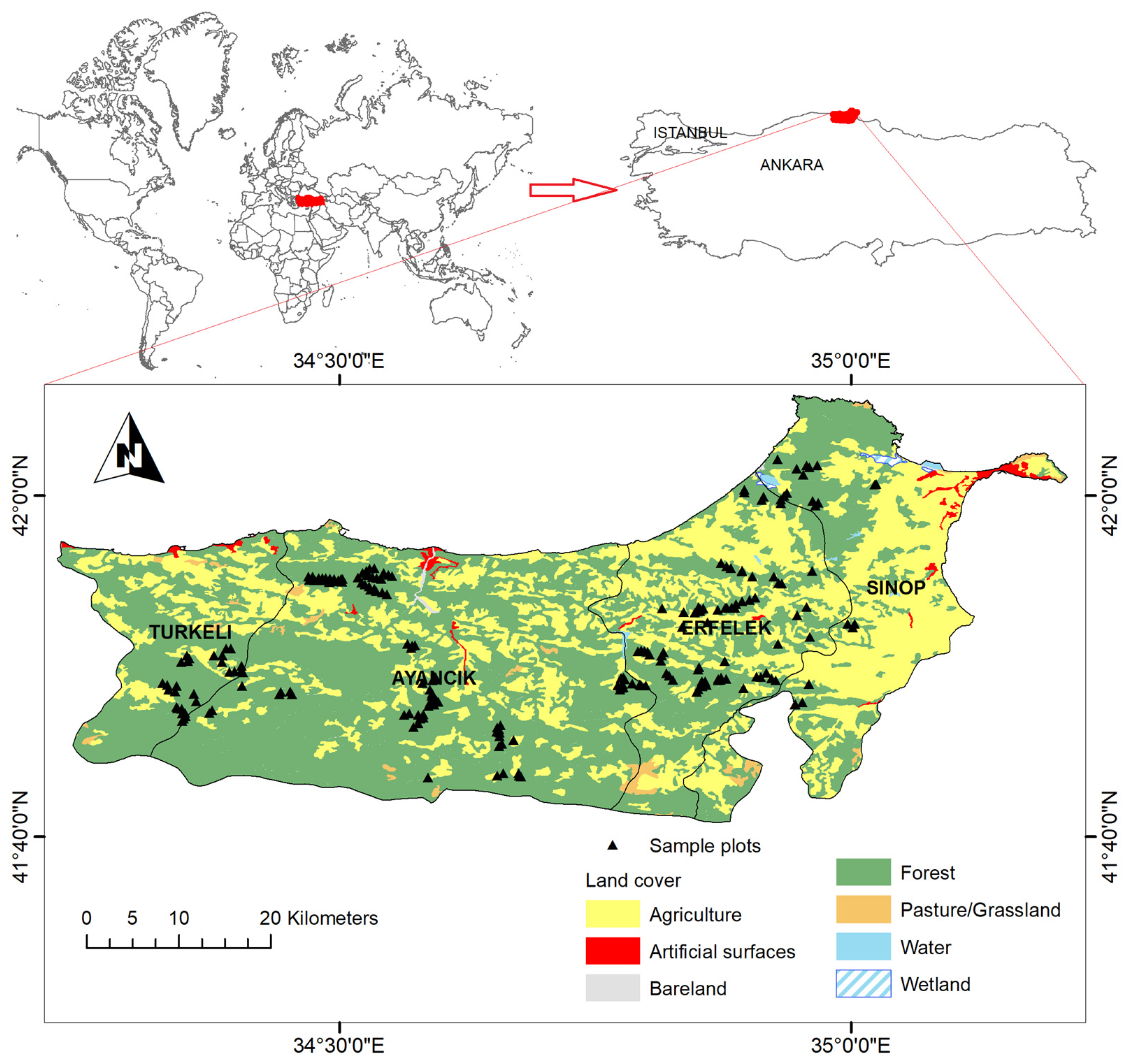
2.1. Site Description

The research area is within the border of Ayancık, Sinop, and Turkeli Forest Enterprises, affiliated with the Sinop Regional Directorate of Forestry. The study area is situated between 41°40′50″–42°05′53″ N latitudes and 34°13′28″–35°12′40″ E longitudes (Figure 1). There is a sharp increase in elevation in the study area, except for the narrow coastal plains in Ayancik. The minimum altitude starts from sea level and reaches 1500–1800 m in the Eastern part of the Mountains İsfendiyar along Sinop Province [32].
The area’s geological structure mainly comprises Upper Cretaceous, Eocene, and Neogene-aged sedimentary rocks and Quarternary-aged marine deposits [33]. There are mostly four great soil groups in the study area according to the USDA soil taxonomy: hapludults, dystrudepts, hapludalfs, and udivitrands affiliated to the order of ultsiols, inceptisols, alfisols, and mollisols, respectively [34]. The climate in Sinop is a typical Black Sea regime: while the mean annual total precipitation ranges from 675 mm to 1012 mm, the mean annual temperature changes between 13.2 °C and 14.1 °C. More than 75% of the annual precipitation falls in the winter and fall. The minimum and maximum mean temperature changes between 7.4–11.0 °C and 16.7–18.6 °C, respectively [35]. The area’s land cover comprises mostly forest (62%) and agricultural lands (35%). The remaining area includes pasture/grasslands, artificial surfaces, water bodies, wetlands, and bare lands (Figure 1).
The vegetation in Sinop is mainly composed of two types: humid forests and pseudo maquis. While the former type includes oriental beech (Fagus orientalis), oak (Quercus sp.), black pine (Pinus nigra), Calabrian pine (Pinus brutia), fir (Abies nordmanniana), and Scotch pine (Pinus sylvestris), the latter includes laurel (Laurus nobilis), Irish strawberry (Arbutus unedo), saunders (Arbutus andrachne), heather (Erica arborea), phllyrea (Phillyrea latifolia), bushy juniper (Juniperus oxycedrus), rockrose (Cistus sp.), and terebinth (Pistacia sp.), along with other fruit trees [37].

2.2. Data Collection and Analyses

2.2.1. Field Data Collection

The study was carried out during the summer seasons of 2008, 2009, and 2011 in the oriental beech stands of the regional forestry directorate. To that end, 222 circular sample plots (0.04 ha) were distributed to the entire area in GIS using a stratified random sampling design [38]. We ensured the sample plots were fully stocked and showed no insect or disease trace.
Some environmental variables regarding topography, climate, and soil were used to predict/model the SDH, computed by taking the average height of four dominant trees. The average age of the stands was calculated by counting four dominant trees’ rings on the cores at breast height (1.3 m) and then adding ten years to each for seedling age [1,39].
The longitude (LONG), latitude (LAT), aspect (ASP), and elevation (ELEV) data were recorded by a handheld GPS, and the ground slope (SLP) was measured using an inclinometer on each plot. The slope position (SPOS) was noted according to the approach described in Schoeneberger’s study [40].
A soil pit was dug up to the bedrock and described according to Cepel’s method [41], and disturbed soil samples were taken from the topsoil (at 0–20 cm soil depth) in each plot. Some physical (sand, silt, and clay content and available water capacity) and chemical (pH, organic carbon, electrical conductivity, and lime) properties were also determined on each sample in addition to measuring the soil depth.
In the next step, the soil samples were transferred to the lab. The soil texture and available water capacity (AWC) were determined following the methods of Bouyoucos [42] and pressure desorption [43]. The soils’ pH and EC, organic carbon (OC), and lime content were determined following the glass electrode, Scheibler [43], and Walkley–Black wet digestion methods, respectively [44].

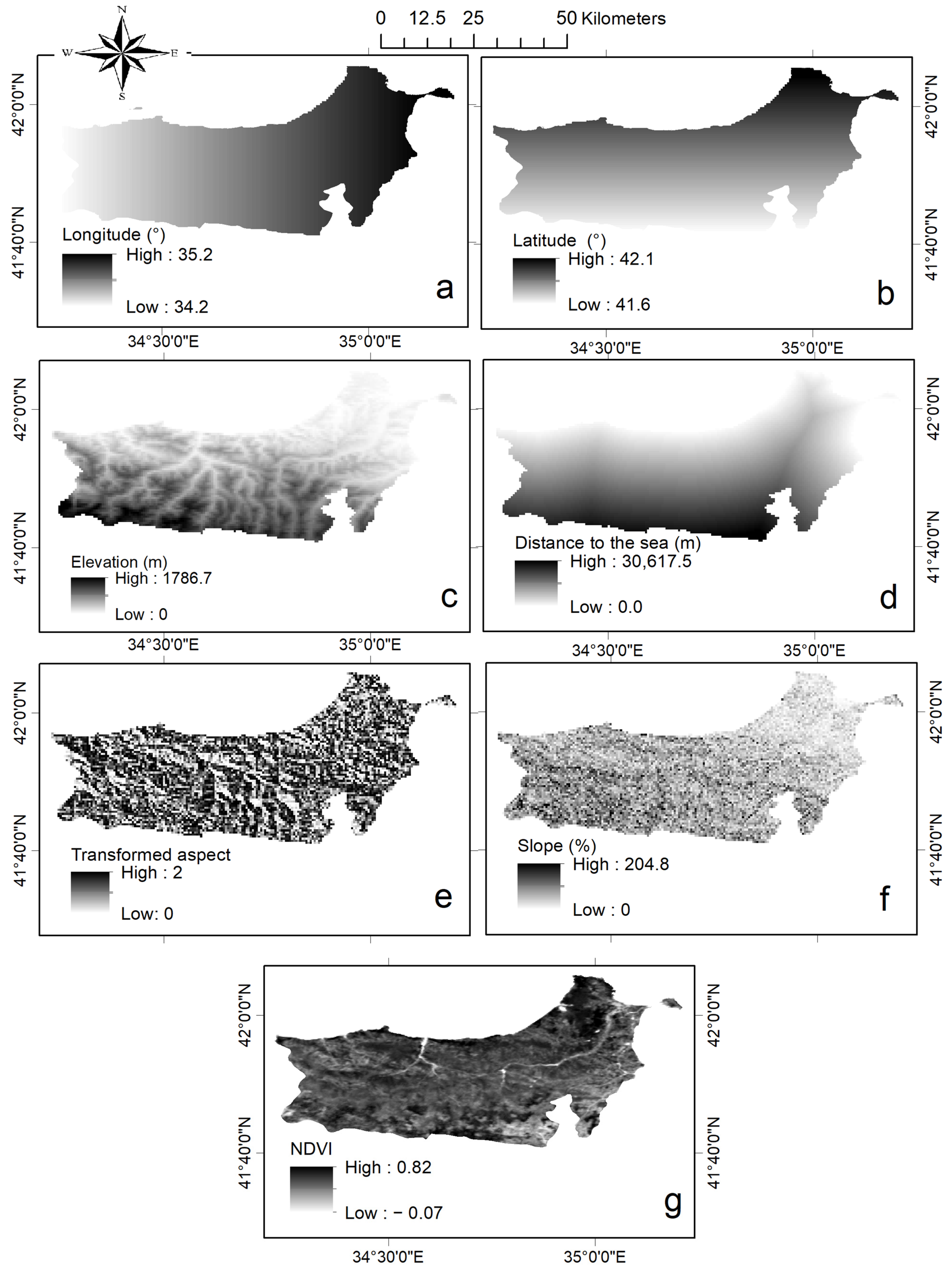
2.2.2. Spatial Data Extraction

We used independent variables extracted from the maps shown in Figure 2 and Figure 3. These maps were generated from various data sources and web platforms, like the DEM and GEE. The LONG, LAT, and ELEV datasets were extracted from the DEM using ArcMap conversion tools (i.e., feature to raster) and spatial analyst tools (i.e., extract values to points). The slope (SLP) and aspect (ASP) values were obtained from the surfaces created using the DEM through the ArcMap spatial analyst tool. Then, the aspect values were transformed to the radiation index (TRASP), ranging from 0.0 on the NNE slopes to 1.0 on the SSW slopes, which was calculated using Equation (1) [45].
TRASP = [1 − cos ((π/180) (ASP − 30))]/2
Additionally, the distance to the sea (DTS) was created using spatial analyst tools (i.e., distance) [46]. The coastline vector dataset was obtained from Kelso and Patterson [47]. The other variable to be correlated to the SDH was the normalized difference vegetation index (NDVI) obtained from NASA using the Google Earth Engine platform (Didan, 2015). The NDVI, calculated by Equation (2), serves as a measure of the quantity, health, and spread of green plants within a region, achieved by assessing the spectral reflectance disparity between the red (Red) and near-infrared (NIR) bands of an image [48]:
NDVI = (NIR − Red)/(NIR + Red)
The climate variables such as the mean annual temperature (MAT), mean annual minimum temperature (MAMINT), mean annual maximum temperature (MAMAXT), and total precipitation (MATP) were extracted from the spatial climate surfaces developed by Yener [49] at a spatial resolution of 0.005° × 0.005° (approximately 600 m). The soil variables, such as the bulk density (BD), OC, field capacity (FC), and pH, were extracted from the maps provided by Hengl and Wheeler [26] and Hengl [27,28].

2.2.3. Analysis and Mapping

First, Pearson’s correlation analysis and partial dependence plots (PDP) were used to analyze the linear and nonlinear relations between the SDH and the other variables. The smoothed PDPs were created for each explanatory variable using the pdp package in the R programming language [50]. The PDPs demonstrated whether each predictor affected the response variable while preserving the average of the remaining predictors [8,14]. After determining the correlations between the variables, MLR and RT analyses were performed to model the SDH using the site variables. While the linear and nonlinear relations were determined using R [51], DTREG was used in the modeling [52].
After the RT and MLR models were developed, potential dominant height maps regarding oriental beech stands were generated using Map Algebra in the spatial analyst tools in ArcMap [46]. In this process, the model equations were entered into the software, and the topographic, climatic, and edaphic surfaces in the raster format were introduced to the program as the independent variables (to be used in equations) and then the tool was run [53,54]. While the resolution of the predicted productivity maps was 0.005, equaling 600 m, the used surfaces’ resolution was 30 m for the topographic, 250 m for the edaphic, and 600 m for the climatic attributes.

3. Results and Discussion

This section presents three subheadings: field-based data, relationships between the stand dominant height (SDH) and spatial data, and predicting and mapping SDH.

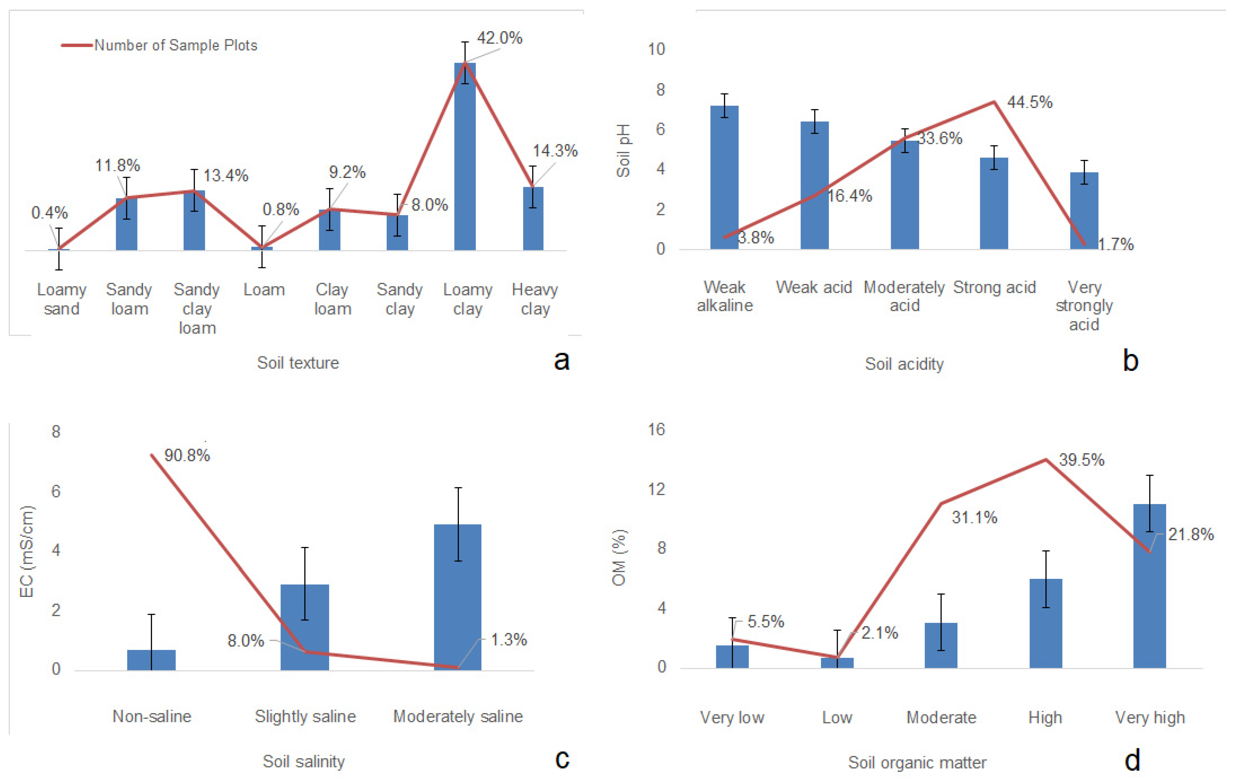
3.1. Field-Based Data

The field data comprised the stand dominant height, stand age, and various soil properties, including the soil depth, texture, available water capacity, pH, electrical conductivity, organic matter, and lime (Table 1). While the oriental beech SDH ranged between 14.6 m and 33.4 m with an average of 22.8 m, the stand ages ranged between 29 and 148 with an average of 73 years. The soil depths across the sample plots changed between 40 and 145 cm, averaging 105.2 cm. Oriental beech is well grown moderate and deep soils [55]. The average soil depth in oriental beech stands ranged from 70 cm to 95.2 cm in other studies [56,57,58,59].
The soil texture in the sampled plots was mainly composed of loamy clay (42.0%), heavy clay (14.3%), sandy clay loam (13.4%), sandy loam (11.8%), and others (18.5%) (Figure 4a).
Changing topography, climate, parent material, and living organisms’ impact shape the soil texture over time. The soil texture of oriental beech forests varies from heavy clay [60] to loam and sandy loam [61].
The pH ranged between 3.8 and 7.4, with an average of 5.3 (Table 1, Figure 4b). Strongly acid soils dominate the study area with an area share of 45% (Figure 4b). The soil pH range in our study is consistent with those reported in other studies [62,63,64,65]. The EC was between 0.1 mS/cm and 6.48 mS/cm, with an average of 0.9 mS/cm. The salinity classes in the study area were formed as non-saline (91%), slightly saline (8%), and moderately saline (1%) (Figure 4c). The soil salinity of beech stands is generally low and characterized as non-saline in most studies [57,60,66]. The soils’ organic matter and lime content were 2–10.5% and 0–17.4%, with an average of 3.4% and 1.9%, respectively (Table 1, Figure 4d). The soil organic matter content classes were characterized as high (39%), moderate (31%), very high (20%), and others (10%) (Figure 4d). Topographic and climatic factors affected the soil OC, along with the soil texture, and the stand characteristics. Therefore, the average OC content of beech stands varied from 1.9–3.0% [61,64] to 3.6–3.9% [55,60,67]. The AWC ranged between 1.9% and 23.3%, with an average of 12.3% (Table 1).

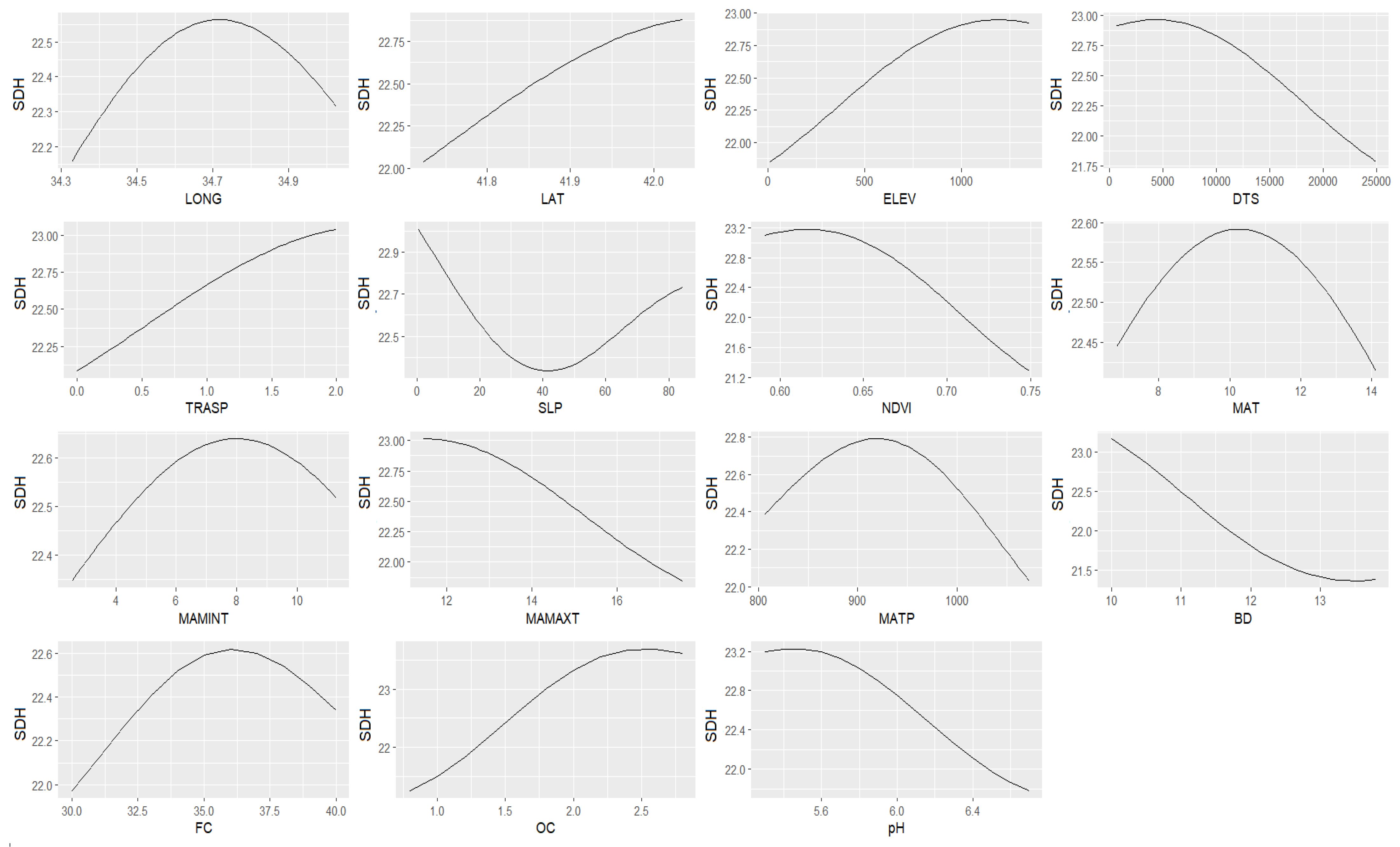
3.2. Relationships between the Stand Dominant Height (SDH) and Spatial Data

This study used digitally extracted data as the explanatory variables to model and map the oriental beech stands’ dominant height. While the Pearson correlation determined the relationships between the SDH and the explanatory variables (Figure 5), the partial dependence plots visualized these relations (Figure 6). The variables included were topographic (i.e., LONG, LAT, ELEV, DTS, TRASP, SLP, and NDVI), climatic (i.e., MAT, MAMINT, MAMAXT, and MATP), and edaphic (i.e., BD, FC, OC, and pH).
Assessing the spatial data retrieved from various resources (Table 1), we saw that our sample plots were located between 34.3°–35.0° N longitudes and 41.7°–42.0° E latitudes. The ELEV ranged from 12 m near sea level to 1352 m with an average of 630.9 m. The average DTS was 12,279 m in the area and reached up to 24,935 m. The slope of the sample plots changed between 5 and 84.4%, with an average of 31.8% corresponding to steep slopes. The NDVI also assessed as part of the topographic variables averaged 0.66, ranging between 0.59 and 0.75, which is relatively high.
Of these variables, the ELEV was positively correlated (r = 0.36), and the LAT (r = −0.25) and NDVI (r = −0.24) were negatively correlated with the SDH. No significant relationships existed with the other topographic variables (p > 0.05) (Figure 5). The DTS, LAT, and ELEV are essential factors in determining the regional climate parameters, such as temperature, precipitation, and radiation, affecting forest productivity [19,68]. While the latitude impacts those parameters’ distribution, increasing the ELEV shortens the growing period due to the decreasing temperature and increases the relative humidity [69]. The negative effect of reducing the ELEV on the SDH could be attributed to the optimum altitudinal zone for the oriental beech stands in Sinop, which is between 600 m and 1200 m with an average of 1000 m [70].
Therefore, increasing the elevation improved the SDH. The altitudinal zone could also explain the negative correlation between the LAT and SDH. This is because increasing the LAT means decreasing the elevation (r = −0.9) (Figure 5). The partial dependency plots, showing nonlinear relations, indicated that the SDH increased with the ELEV increasing up to 1000 m and then decreased (Figure 6), which could be proof of the optimum altitudinal zone being below 1000 m for oriental beech stands. Similar results on the effect of the ELEV on stand productivity were found in other studies [7,12,14,58,71]. For example, Alavi et al. [7] also attributed increased productivity in oriental beech stands of Hyrcania, Iran, to increasing the ELEV to the optimum altitudinal zone, above 1500 m. Güner et al. [72] linked this positive effect of the ELEV on Anatolian black pine productivity to improved precipitation at higher altitudes. However, other authors [4,14,15] reported conflicting findings due to deteriorated ecological conditions with increasing ELEV, such as shortening the growing period, decreasing fine-textured soil, and reducing decomposition due to the condensing temperature. The reducing effect of LAT on stand productivity was also reported in some studies [14,73]. Klinka et al. [73] reported a decrease of 2.9 m in the Norway spruce SI and 2.5 m in the Douglas fir SI with a 1° increase in latitude and 100 m in elevation.
Another topographic variable correlated with the SDH was the NDVI, whose relatively higher value above 0.6 in the study area indicates dense vegetation cover. Its weak negative correlations with the SDH could also be linked to somewhat higher altitudes (r = −0.69 between the NDVI and ELEV, Figure 5), regarded as the oriental beech’s growing optimum. It is also associated with decreasing precipitation in beech sites due to going southward, negatively affecting the NDVI (r = 0.76 between the NDVI and LAT, Figure 3d and Figure 5) [74,75]. On the contrary, some other researchers found positive correlations between the NDVI and site productivity [21,22,76,77,78].
The climatic variables used in this study were extracted from the climate surfaces developed by Yener [49]. According to this dataset, the study area’s climate is characterized by an average of 10.6 °C mean, 7.0 °C mean minimum, and 14.8 °C mean maximum temperatures with minimum–maximum values of 6.8–14.1 °C, 2.5–11.3 °C, and 11.5–17.5 °C, respectively (Table 1, Figure 3a–c). The precipitation in the study area ranged from 806.4 mm to 1072.9 mm and averaged 925.4 mm (Table 1, Figure 3d). Climate, one of the main ecological factors affecting terrestrial ecosystems at global and local scales, is the driving force for the biogeochemical cycle in nature [17,69]. Variable climatic conditions also affect biomass and soil litter decomposition and carbon accumulation [79]. Therefore, the MAT, MAMINT, MAMAXT, and MATP were used in this study; however, the MAMAXT was the only climatic factor significantly correlated with the SDH (r = −0.39) (Figure 5).
Our finding is similar to those reported in other studies [12,13,80,81]. The negative effect of the MAMAXT on the SDH may be attributed to enhanced summer drought [80]. Seltmann et al. [13] reported improved Norway spruce growth because of the low temperature and high AWC. However, the temperature in most studies [14,15,82,83] positively affected tree growth, attributed to prolonged growing periods, enhancing microbial activities and improving decomposition and soil attributes. Although no significant effect of precipitation on the SDH was observed in this study, some other studies [13,72,80,81,83] reported that it somehow affects stand productivity. Likewise, we detected no significant climatic variables, except for the MAMAXT. The partial dependence plots (Figure 6) showed that the SDH increased with an increasing MAT and MAMINT and MATP up to about 10 °C, 8 °C, and 950 mm, respectively, and then suddenly decreased.
The digitally extracted BD, FC, OC, and pH averaged 11.5 kg/m3, 33.5%, 1.6%, and 6.0, respectively, and ranged between 10.0 and 13.8 kg/m3, 30 and 40%, 0.8 and 2.8%, and 5.3 and 6.7, respectively (Table 1, Figure 3e–h). All the digitally extracted edaphic variables significantly affected the SDH: while the BD (r = −0.34) and pH (−0.25) were negatively associated with the SDH, the FC (r = 0.26) and OC (r = 0.43) positively affected it (Figure 5).
The positive effect of the FC or FC-based AWC on stand productivity was reported in other studies [8,13,58,59]. Soil moisture or water is one of the most important ecological factors affecting plant growth, especially in influencing soil temperature, aeration, microbial activity, and nutrient availability and diminishing the toxic material concentrations, besides directly providing water to the plants [84]. The situation in which the OC was positively correlated with the SDH could be attributed to the provided functions of organic matter on soil quality through an increased cation exchange and available water capacity, improving soil aggregates, aeration, and porosity and providing nutrients [85,86]. Similar findings were reported by Aertsen et al. [87] and Subedi and Fox [88]. Results, in contrast to ours, were also found by some other researchers [4,58], attributing their outcomes to decreased pH with increasing organic matter. Unlike the FC and OC, the BD and pH negatively affected productivity in the present study. An indicator of soil acidity, pH mainly affects some processes, such as nutrient availability, nitrification, microbial activity, and heavy metal toxicity [89]. Most of the studies [71,87,88] reported a positive effect of pH on productivity, attributing it to improving soil conditions, such as nutrient availability and microbial activity. However, some other researchers [7,64] reported contrasting results in disagreement with our study. Our results showed that pH is one of the limiting factors for the dominant height growth of oriental beech. An increasing pH negatively affects some elements’ availability in the soil solution, such as phosphorus, iron, zinc, and manganese [7]. The BD is calculated by summing the soil pores and solids to the soil volume; its unit is gr/cm3. A low BD indicates a loose and highly porous structure due to the high organic matter in soils [86], consistent with our finding in Figure 5, showing r = −0.7 between the BD and OC. Increases in BD generally result in adverse effects on tree development through the negatively affected mentioned soil properties [90]. As a matter of fact, Irmak [91] and Cepel [41] stated that the effect of soil properties on stand development becomes more evident when the climate is not very variable, and the species moves away from the optimum conditions.

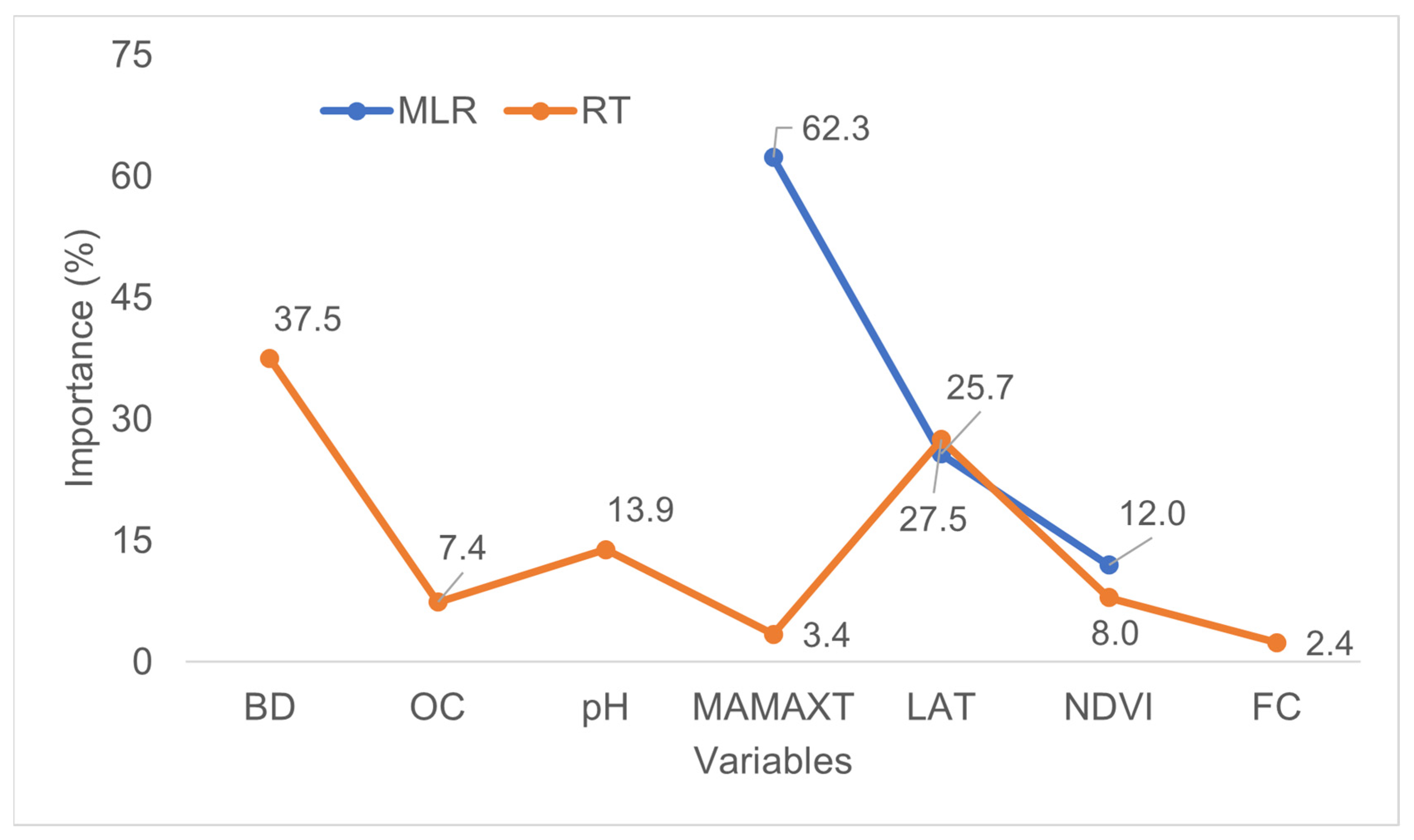
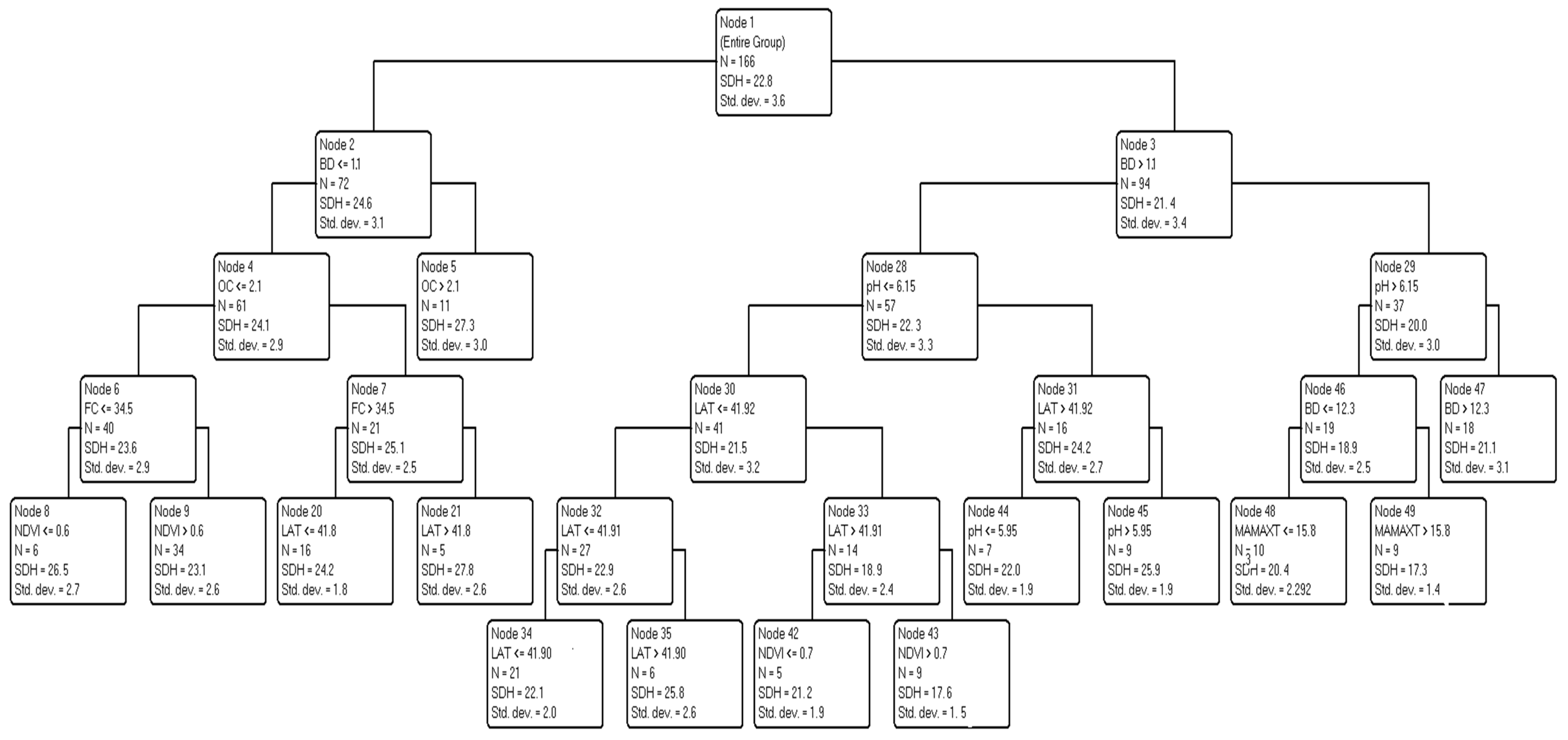
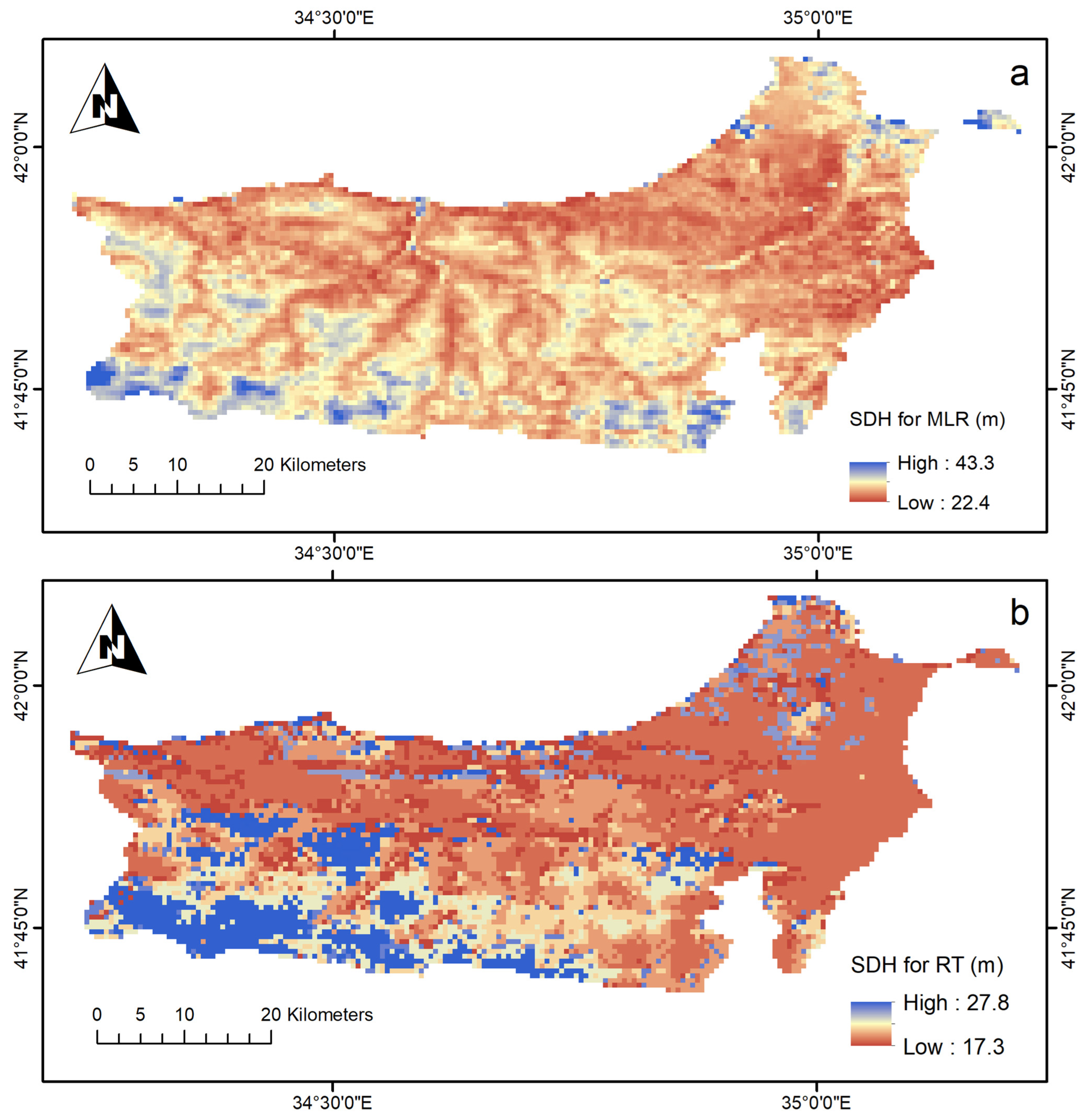
3.3. Predicting and Mapping SDH

The presented study aimed to predict the SDH from spatial data, including topographic, climatic, and edaphic variables, using MLR and RT analyses and then generating potential SDH maps using those models. We randomly selected 75% of the sample plots as the training datasets in this context, withholding the remaining 25% as validation. The model results showed that MLR accounted for 26% and 21% of the variation in the SDH, with an RMSE of 3.16 m and 3.27 m for training and validation, respectively. RT outperformed MLR, explaining 57% and 25% of the variation, with an RMSE of 2.37 m and 3.33 m for training and validation, respectively (Figure 7). The RT model included at least one variable from any group, such as topographic, climatic, and edaphic; however, MLR included only climatic and topographic variables.
The most critical variable in the models was MAMAXT for MLR and BD for RT, with an importance of 62.3% and 37.5%. The most critical factor group affecting the SDH was the climate, with an importance rate of 62.3%, and the soil, with an importance rate of 61.2% for the MLR and RT models (Figure 8).
Many studies [4,12,15,16,71,72,82,92] have used MLR and RT for estimating forest productivity. Our model results are consistent with those reported in other studies [4,5,12,15,72,92,93,94]. The most satisfied results in these outperformed models were reached as an adjusted R2 of 0.85 and RMSE of 1.17 m for the training dataset and an R2 of 0.54 and RMSE of 1.91 m for validation by Alavi et al. [7] in the Hyrcanian oriental beech forests of Iran using edaphic and physiographic variables. Mohammadi et al. [5] also predicted oriental beech productivity, e.g., stand volume using MLR and RT techniques, and RT outperformed with an R2 of 0.67 (percentage RMSE = 30%). Some other statistical approaches have also been implemented to model forest productivity, such as the complementary methodological approach [95], random forest analysis [14,96,97], Chapman–Richards model [83,98], and linear mixed effects models [99].
In an RT analysis, a particular site productivity indicator, such as the dominant height and site index, is classified by considering the predictors (independent or explanatory variables). The precise value of the predictor optimally splits the data at any branch of the tree [100].
The RT model in this study included seven independent variables: edaphic (BD, pH, OC, and FC), topographic (LAT and NDVI), and climatic (MAMAXT). The soil BD, with a variable importance of 37.5%, followed by the LAT (18.5%) and pH (13.9%) (Figure 8 and Figure 9), is the first and primary variable controlling the SDH. At this point, a BD below or equal to 1.1 gr/cm3 resulted in an SDH of 24.6 m. However, a BD above that value corresponded to an SDH of 21.4 m., which was 13% lower than the previous one, suggesting that a decreased BD (below 1.1 gr/cm3) improves the SDH. The second important node was an LAT above 41.8° interacting with a BD equal to or below 1.1 gr/cm3, an OC equal to or below 2.1%, and an FC above 34.5%, resulting in a 27.8 m SDH, the highest value in this model followed by the BD (equal to or below 1.1 gr/cm3) and OC (above 2.1%) interactions corresponding to the 27.2 m SDH.
This RT model suggests that it is vital to establish oriental beech stands where the BD is below 1.1 gr/cm3 and the OC is above 2.1%, or the BD is equal to or below 1.1 gr/cm3, the OC is equal to or below 2.1%, the FC is above 34.5%, and the LAT is above 41.8°. It also suggests that the sites with a relatively higher BD (>1.1 gr/cm3) with a pH equal to or below 6.15 and an LAT below 41.9° are more productive than sites with more than 6.15 pH.
Afif-Khouri et al. [71] and Menendez-Miguelez et al. [82] also used RT to predict the stand productivity in NW Spain chestnut coppice stands. While extractable Mg and annual temperature were the only determinants in the former study, the latter research determined the clay content of soils and the spring and summer precipitation as nodes in the RT. On the other hand, the MLR model comprises the MAMAXT, LAT, and NDVI, which were also included in the RT model.
We also mapped the potential productivity of the oriental beech forest in the study area. The resolution of the maps shown in Figure 10 is 0.005° (600 m/pix). According to the maps, the stand dominant height was between 22.4 and 43.3 m for MLR and 17.3 and 27.8 m for the RT model. However, with some differences in the model maps, the productivity increases toward the area’s inner part, especially to the southwest (Figure 10). This improvement could be explained by enhanced ecological conditions in this part, such as an elevated OC (Figure 3g) and FC (Figure 3f), a decreased BD (Figure 3e), and reaching the optimum altitudinal zone in terms of air temperature (Figure 2c), suggesting that coastal areas are unsuitable for oriental beech in this region.
The other point is decreased productivity in the region’s eastern part, which can be attributed to the increased temperatures and decreased organic matter. Other researchers [6,23,101,102,103] have also mapped forest productivity at variable spatial resolutions, ranging from 5 m to 1000 m. They used soil, climate, and terrain attributes based on different statistical techniques, like RF, RT, Chapman–Richards, and MLR. While Swenson et al. [103] predicted and mapped the SI for Douglas fir stands with an R2 of 0.55 and RMSE of 6.1 m in the USA, Jiang et al. [101] found those values to be an R2 of 0.64 and RMSE of 4.6 m for softwood and an R2 of 0.36 and RMSE of 4.2 m for hardwood species also in the USA.

4. Conclusions

Because there is insufficient knowledge of the spatial variation of species-specific site productivity, generating dominant height maps is crucial for forest management practices, such as reforestation and plantation. The maps generated in this study could help forest planners and land managers visualize the most productive oriental beech sites rapidly. Our approach can also be used in locations with different vegetation types if site-specific spatial data are available.
Based on the results, it is concluded that the RT model outperformed the MLR model with more accurate estimates and maps. The RT model emphasizes that edaphic factors should be given more importance than others, particularly in oriental beech afforestation and reforestation works. Using freely available spatial datasets with more spectral data and the RT technique, researchers can develop new site productivity models and generate wall-to-wall maps of their area of investigation. Thus, site productivity can be assessed in a spatially explicit manner.

Author Contributions

E.G.—field and laboratory studies, writing and reviewing; I.Y.—original draft preparation, methodology, statistical analyses and mapping with GIS, writing, reviewing and editing. All authors have read and agreed to the published version of the manuscript.

Funding

This work was supported by the TÜBİTAK—TOVAG (The Scientific and Technological Research Council of Turkey—Research Committee of Agriculture, Forestry and Veterinary), with Project Number: 107O752.

Institutional Review Board Statement

Not applicable.

Informed Consent Statement

Not applicable.

Data Availability Statement

Not applicable.

Acknowledgments

Some of the data used in this study were obtained from the doctoral thesis of the second author. The authors thank Can Vatandaslar for his valuable English editing. We also acknowledge the reviewers and the journal editors for their helpful comments and suggestions to improve the manuscript.

Conflicts of Interest

The authors declare no conflict of interest. The funders had no role in the design of the study; in the collection, analyses, or interpretation of the data; in the writing of the manuscript; or in the decision to publish the results.

References

  1. Skovsgaard, J.P.; Vanclay, J.K. Forest site productivity: A review of the evolution of dendrometric concepts for even-aged stands. Forestry 2008, 81, 13. [Google Scholar] [CrossRef]
  2. García, O.; Batho, A. Top Height Estimation in Lodgepole Pine Sample Plots. West. J. Appl. For. 2005, 20, 64–68. [Google Scholar] [CrossRef]
  3. Noordermeer, L.; Gobakken, T.; Næsset, E.; Bollandsås, O.M. Predicting and mapping site index in operational forest inventories using bitemporal airborne laser scanner data. For. Ecol. Manag. 2020, 457, 117768. [Google Scholar] [CrossRef]
  4. Yener, I.; Altun, L. Predicting Site Index for Oriental Spruce (Picea orientalis L. (Link)) Using Ecological Factors in the Eastern Black Sea, Turkey. Fresenius Environ. Bull. 2018, 27, 3107–3116. [Google Scholar]
  5. Mohammadi, J.; Shataee, S.; Babanezhad, M. Estimation of forest stand volume, tree density and biodiversity using Landsat ETM plus Data, comparison of linear and regression tree analyses. Procedia Environ. Sci. 2011, 7, 299–304. [Google Scholar] [CrossRef]
  6. Laamrani, A.; Valeria, O.; Bergeron, Y.; Fenton, N.; Cheng, L.Z.; Anyomi, K. Effects of topography and thickness of organic layer on productivity of black spruce boreal forests of the Canadian Clay Belt region. For. Ecol. Manag. 2014, 330, 144–157. [Google Scholar] [CrossRef]
  7. Alavi, S.J.; Ahmadi, K.; Dormann, C.; Serra-Diaz, J.M.; Nouri, Z. Assessing the dominant height of oriental beech (Fagus orientalis L.) in relation to edaphic and physiographic variables in the Hyrcanian Forests of Iran. Biotechnol. Agron. Soc. Environ. 2020, 24, 262–273. [Google Scholar] [CrossRef]
  8. Littke, K.M.; Harrison, R.B.; Zabowski, D. Determining the Effects of Biogeoclimatic Properties on Different Site Index Systems of Douglas-fir in the Coastal Pacific Northwest. For. Sci. 2016, 62, 503–512. [Google Scholar] [CrossRef]
  9. Ozkan, K. Modelling ecological data using classification and regression tree technique (CART). Turk. J. For. 2012, 13, 1–4. [Google Scholar]
  10. Prasad, A.M.; Iverson, L.R.; Liaw, A. Newer Classification and Regression Tree Techniques: Bagging and Random Forests for Ecological Prediction. Ecosystems 2006, 9, 181–199. [Google Scholar] [CrossRef]
  11. Yuan, Z.Q.; Ali, A.; Wang, S.P.; Gazol, A.; Freckleton, R.; Wang, X.G.; Lin, F.; Ye, J.; Zhou, L.; Hao, Z.Q.; et al. Abiotic and biotic determinants of coarse woody productivity in temperate mixed forests. Sci. Total Environ. 2018, 630, 422–431. [Google Scholar]
  12. Gulsoy, S.; Cinar, T. The Relationships between Environmental Factors and Site Index of Anatolian Black Pine (Pinus Nigra Arn. Subsp. Pallasiana (Lamb.) Holmboe) Stands in Demirci (Manisa) District, Turkey. Appl. Ecol. Environ. Res. 2019, 17, 1235–1246. [Google Scholar] [CrossRef]
  13. Seltmann, C.T.; Wernicke, J.; Petzold, R.; Baumann, M.; Munder, K.; Martens, S. The relative importance of environmental drivers and their interactions on the growth of Norway spruce depends on soil unit classes: A case study from Saxony and Thuringia, Germany. For. Ecol. Manag. 2021, 480, 118671. [Google Scholar] [CrossRef]
  14. Zhang, H.Y.; Feng, Z.K.; Wang, S.; Ji, W.X. Disentangling the Factors that Contribute to the Growth of Betula spp. and Cunninghami lanceolata in China Based on Machine Learning Algorithms. Sustainability 2022, 14, 8346. [Google Scholar] [CrossRef]
  15. Velioglu, E.; Guener, S.T.; Karakurt, H.; Tastan, Y.; Yavuz, Z.; Tugrul, D. Relationships between site index and ecological variables of trembling poplar forests (Populus tremula L.) in Turkiye. Environ. Monit. Assess. 2023, 195, 308. [Google Scholar]
  16. Aertsen, W.; Kint, V.; van Orshoven, J.; Ozkan, K.; Muys, B. Comparison and ranking of different modelling techniques for prediction of site index in Mediterranean mountain forests. Ecol. Model. 2010, 221, 1119–1130. [Google Scholar] [CrossRef]
  17. Orlandini, S.; Bindi, M.; Howden, M. Plant biometeorology and adaptation. In Biometeorology for Adaptation to Climate Variability and Change; Springer: Berlin/Heidelberg, Germany, 2009; pp. 107–129. [Google Scholar]
  18. Pan, Y.; Birdsey, R.A.; Phillips, O.L.; Jackson, R.B. The structure, distribution, and biomass of the world’s forests. J. Annu. Rev. Ecol. Evol. Syst. 2013, 44, 593–622. [Google Scholar]
  19. Stage, A.R.; Salas, C. Interactions of elevation, aspect, and slope in models of forest species composition and productivity. For. Sci. 2007, 53, 486–492. [Google Scholar]
  20. Becknell, J.M.; Powers, J.S. Stand age and soils as drivers of plant functional traits and aboveground biomass in secondary tropical dry forest. Can. J. For. Res. 2014, 44, 604–613. [Google Scholar] [CrossRef]
  21. Brito, V.V.; Rubilar, R.A.; Cook, R.L.; Campoe, O.C.; Carter, D.R.; Mardones, O. Evaluating remote sensing indices as potential productivity and stand quality indicators for Pinus radiata plantations. Sci. For. 2021, 49, e3316. [Google Scholar] [CrossRef]
  22. Gazol, A.; Rozas, V.; Arribas, S.C.; Ponce, R.A.; Rodriguez-Puerta, F.; Gomez, C.; Olano, J.M. Stand characteristics modulate secondary growth responses to drought and gross primary production in Pinus halepensis afforestation. Eur. J. For. Res. 2023, 142, 353–366. [Google Scholar]
  23. Zushi, K. Regional estimation of Japanese cedar (Cryptomeria japonica D. Don) productivity by use of digital terrain analysis. J. For. Res. 2007, 12, 289–297. [Google Scholar] [CrossRef]
  24. NASA/METI/AIST, Japan Spacesystems and U.S./Japan ASTER Science Team. ASTER Global Digital Elevation Model [Data Set]. 2019. Available online: https://lpdaac.usgs.gov/products/astgtmv003/ (accessed on 9 September 2022).
  25. Hijmans, R.J.; Cameron, S.E.; Parra, J.L.; Jones, P.G.; Jarvis, A. Very high resolution interpolated climate surfaces for global land areas. Int. J. Climatol. 2005, 25, 1965–1978. [Google Scholar] [CrossRef]
  26. Hengl, T.; Wheeler, I. Soil Organic Carbon Content in x 5 g/kg at 6 Standard Depths (0, 10, 30, 60, 100 and 200 cm) at 250 m Resolution (Version v02) [Data Set]; Zenodo: Geneva, Switzerland, 2018. [Google Scholar]
  27. Hengl, T. Clay Content in % (kg/kg) at 6 Standard Depths (0, 10, 30, 60, 100 and 200 cm) at 250 m Resolution (Version v02) [Data Set]; Zenodo: Geneva, Switzerland, 2018. [Google Scholar]
  28. Hengl, T. Soil Bulk Density (Fine Earth) 10 x kg/m-Cubic at 6 Standard Depths (0, 10, 30, 60, 100 and 200 cm) at 250 m Resolution (Version v02) [Data Set]; Zenodo: Geneva, Switzerland, 2018. [Google Scholar]
  29. Xu, C.; Du, X.; Jian, H.; Dong, Y.; Qin, W.; Mu, H.; Yan, Z.; Zhu, J.; Fan, X. Analyzing large-scale Data Cubes with user-defined algorithms: A cloud-native approach. Int. J. Appl. Earth Obs. Geoinf. 2022, 109, 102784. [Google Scholar] [CrossRef]
  30. OGM. Ormanlarımızda Yayılış Gösteren Asli Ağaç Türleri; Orman Genel Müdürlüğü: Ankara, Turkey, 2009; p. 48. [Google Scholar]
  31. OGM, Orman Varlığımız. TC Çevre Ve Orman Bakanlığı; Orman Genel Müdürlüğü Yayınları: Ankara, Turkey, 2020. [Google Scholar]
  32. Guvendi, E. Saf Doğu Kayını (Fagus orientalis Lipsky.) Ormanlarının Ekolojik Tabanlı İdare Sürelerinin Belirlenmesi (Sinop-Ayancık-Türkeli Örneği). Ph.D. Thesis, Karadeniz Technical University, Trabzon, Türkiye, 2013. [Google Scholar]
  33. MTA. Geological Map of Turkey; General Directorate of Mineral Research and Exploration: Ankara, Turkey, 2019. [Google Scholar]
  34. Hengl, T.; Nauman, T. Predicted USDA SOIL Great Groups at 250 m (Probabilities), v01; Zenodo: Geneva, Switzerland, 2018. [Google Scholar]
  35. Özdemir, N. One of the effective natural disaster in Sinop: The landslide. Dicle Univ. J. Ziya Gökalp Fac. Educ. 2005, 5, 67–106. [Google Scholar]
  36. Cover Corine Land, European Union, Copernicus Land Monitoring Service. 2018. Available online: https://sdi.eea.europa.eu/catalogue/copernicus/api/records/71c95a07-e296-44fc-b22b-415f42acfdf0?language=all (accessed on 9 September 2022).
  37. Yıldız, S. Sinop ve Çevresinin Bitki Örtüsü. Master’s Thesis, Istanbul University, Istanbul, Türkiye, 2000. (In Turkish). [Google Scholar]
  38. Pennock, D.; Yates, T.; Braidek, J. Soil sampling designs. Soil Sampl. Methods Anal. 2008, 2, 25–37. [Google Scholar]
  39. van Laar, A.; Akça, A. Forest Mensuration; Springer: Dordrecht, The Netherlands, 2007. [Google Scholar]
  40. Schoeneberger, P.J. Field Book for Describing and Sampling Soils; National Soil Survey Center, Natural Resources Conservation Service, U.S. Department of Agriculture: Lincoln, NE, USA, 2002.
  41. Cepel, N. Forest Ecology; Istanbul University, Faculty of Forestry: İstanbul, Turkey, 1978. [Google Scholar]
  42. Bouyoucos, G.J. Hydrometer method improved for making particle size analyses of soils. Agron. J. 1962, 54, 464–465. [Google Scholar] [CrossRef]
  43. Kalra, Y.P.; Maynard, D.G. Methods Manual for Forest Soil and Plant Analysis; Forestry Canada, Northwest Region, Northern Forestry Centre: Edmonton, AB, Canada, 1991; p. 116. [Google Scholar]
  44. Walkley, A. A critical examination of a rapid method for determining organic carbon in soils-Effect of variations in digestion conditions and of inorganic soil constituents. Soil Sci. 1947, 63, 251–264. [Google Scholar] [CrossRef]
  45. Bolton, D.K.; White, J.C.; Wulder, M.A.; Coops, N.C.; Hermosilla, T.; Yuan, X. Updating stand-level forest inventories using airborne laser scanning and Landsat time series data. Int. J. Appl. Earth Obs. Geoinf. 2018, 66, 174–183. [Google Scholar] [CrossRef]
  46. ESRI. ArcMap 10.2, 10.2; ESRI: Redlands, CA, USA, 2014. [Google Scholar]
  47. Kelso, N.V.; Patterson, T. Natural earth vector. Cartogr. Perspect. 2009, 64, 45–50. [Google Scholar] [CrossRef]
  48. Tucker, C.J. Red and photographic infrared linear combinations for monitoring vegetation. Remote Sens. Environ. 1979, 8, 127–150. [Google Scholar] [CrossRef]
  49. Yener, İ. Development of high-resolution annual climate surfaces for Turkey using ANUSPLIN and comparison with other methods. Atmósfera 2022, 37, 425–444. [Google Scholar] [CrossRef]
  50. Greenwell, B.M. pdp: An R package for constructing partial dependence plots. R J. 2017, 9, 421. [Google Scholar] [CrossRef]
  51. Team, R.C. R: A Language and Environment for Statistical Computing; R Foundation for Statistical Computing: Vienna, Austria, 2013. [Google Scholar]
  52. Sherrod, P.H. DTREG Predictive Modeling Software. 2020. Available online: http://www.dtreg.com (accessed on 9 September 2022).
  53. Tomlin, C.D. Geographic Information Systems and Cartographic Modeling; Prentice Hall: Englewood Cliffs, NJ, USA, 1990; Volume 249. [Google Scholar]
  54. Tomlin, C.D. Map algebra: One perspective. Landsc. Urban Plan. 1994, 30, 3–12. [Google Scholar] [CrossRef]
  55. Yıldız, O.; Bircan, Ş. Batı Karadeniz kıyı bölgesi’nde yetişen Kayın (Fagus orientalis Lipsky) odununun fiziksel ve mekanik özelliklerinin yetişme ortamı değişkenleriyle ilişkisi. Anadolu Orman Araştırmaları Derg. 2022, 8, 61–72. [Google Scholar] [CrossRef]
  56. Göl, C.; Çelik, N.; Çakır, M.; Gül, E. Türkmen Dağı (Evkondu Tepe) doğu kayını (Fagus orientalis Lipsky.) ormanlarının bazı yetişme ortamı özellikleri. Süleyman Demirel Üniversitesi Orman Fakültesi Derg. Seri A 2008, 1, 48–60. [Google Scholar]
  57. Özel, H.; Ertekin, M. Ecological conditions in the natural group regeneration areas of oriental beech (Fagus orientalis Lipsky.) in Bartın and Devrek district. Bartın Orman Fakültesi Derg. 2010, 12, 47–64. [Google Scholar]
  58. Yılmaz, M. Effects of soil and environmental factors on the site productivity of pure Oriental beech forests in Akkuş Region of Turkey. Eurasian J. For. Sci. 2019, 7, 107–120. [Google Scholar]
  59. Yilmaz, M.; Usta, A.; Ozturk, I. Relationships between site productivity and environmental variables of Oriental beech forests in northeastern Turkey. Austrian J. For. Sci. 2022, 139, 239–262. [Google Scholar]
  60. Bolat, I.; Kara, O.; Tunay, M. Seasonal Changes of Microbial Biomass Carbon, Nitrogen, and Phosphorus in Soil Under an Oriental Beech Stand. Forestist 2022, 72, 259–265. [Google Scholar] [CrossRef]
  61. Azaryan, M.; Vajari, K.A.; Amanzadeh, B. Soil properties and fine root morphological traits in relation to soil particle-size fractions in a broad-leaved beech (Fagus orientalis Lipsky) forest. Acta Oecologica 2022, 117, 103852. [Google Scholar]
  62. Akbas, M.; Tufekcioglu, A. Contribution of the Root Component to Soil Respiration in Oriental Beech Stands in Artvin, Turkey. For. Sci. 2022, 68, 399–409. [Google Scholar]
  63. Amolikondori, A.; Vajari, K.A.; Feizian, M.; Di Iorio, A. Influences of forest gaps on soil physico-chemical and biological properties in an oriental beech (Fagus orientalis L.) stand of Hyrcanian forest, north of Iran. Iforest-Biogeosci. For. 2020, 13, 124–129. [Google Scholar] [CrossRef]
  64. Guner, S.T. Relatıonshıps between Sıte Index and Ecologıcal Varıables of Orıental Beech Forest in the Marmara Regıon of Turkey. Fresenius Environ. Bull. 2021, 30, 6920–6927. [Google Scholar]
  65. Mohammadi, M.F.; Jalali, S.G.; Kooch, Y.; Said-Pullicino, D. The effect of landform on soil microbial activity and biomass in a Hyrcanian oriental beech stand. Catena 2017, 149, 309–317. [Google Scholar] [CrossRef]
  66. Kooch, Y.; Parsapour, M.K.; Egli, M.; Moghimian, N. Forest floor and soil properties in different development stages of Oriental beech forests. Appl. Soil Ecol. 2021, 161, 103823. [Google Scholar]
  67. Bakhshandeh-Navroud, B.; Vajari, K.A.; Pilehvar, B.; Kooch, Y. The interactions between tree-herb layer diversity and soil properties in the oriental beech (Fagus orientalis Lipsky) stands in Hyrcanian forest. Environ. Monit. Assess. 2018, 190, 425. [Google Scholar] [CrossRef]
  68. Bailey, R.G. Ecosystem Geography: From Ecoregions to Sites; Springer Science & Business Media: Berlin/Heidelberg, Germany, 2009. [Google Scholar]
  69. Spurr, S.H.; Barnes, B.V. Forest Ecology; Wiley: Hoboken, NJ, USA, 1991. [Google Scholar]
  70. Atalay, İ. Türkiye’nin Ekolojik Bölgeleri (Ecoregions of Turkey); TC Orman Bakanlığı Yayını: Ankara, Turkey, 2002. [Google Scholar]
  71. Afif-Khouri, E.; Alvarez-Alvarez, P.; Fernandez-Lopez, M.J.; Oliveira-Prendes, J.A.; Camara-Obregon, A. Influence of climate, edaphic factors and tree nutrition on site index of chestnut coppice stands in north-west Spain. Forestry 2011, 84, 385–396. [Google Scholar] [CrossRef]
  72. Güner, Ş.T.; Comez, A.; Ozkan, K.; Karatas, R.; Celik, N. Modelling the productivity of Anatolian black pine plantations in Turkey. Istanb. Univ. Fac. For. 2016, 66, 159–172. [Google Scholar]
  73. Klinka, K.; Wang, Q.; Carter, R.E.; Chen, H.Y.H. Height growth-elevation relationships in subalpine forests of interior British Columbia. For. Chron. 1996, 72, 193–198. [Google Scholar] [CrossRef]
  74. Jiao, K.W.; Gao, J.B.; Liu, Z.H. Precipitation Drives the NDVI Distribution on the Tibetan Plateau While High Warming Rates May Intensify Its Ecological Droughts. Remote Sens. 2021, 13, 1305. [Google Scholar] [CrossRef]
  75. Shi, L.; Fan, H.J.; Yang, L.Y.; Jiang, Y.T.; Sun, Z.H.; Zhang, Y.L. NDVI-based spatial and temporal vegetation trends and their response to precipitation and temperature changes in the Mu Us Desert from 2000 to 2019. Water Sci. Technol. 2023, 88, 430–442. [Google Scholar] [CrossRef] [PubMed]
  76. Bollandsas, O.M.; Orka, H.O.; Dalponte, M.; Gobakken, T.; Naesset, E. Modelling Site Index in Forest Stands Using Airborne Hyperspectral Imagery and Bi-Temporal Laser Scanner Data. Remote Sens. 2019, 11, 1020. [Google Scholar] [CrossRef]
  77. Wang, J.; Rich, P.M.; Price, K.P.; Kettle, W.D. Relations between NDVI and tree productivity in the central Great Plains. Int. J. Remote Sens. 2004, 25, 3127–3138. [Google Scholar] [CrossRef]
  78. Erasmi, S.; Klinge, M.; Dulamsuren, C.; Schneider, F.; Hauck, M. Modelling the productivity of Siberian larch forests from Landsat NDVI time series in fragmented forest stands of the Mongolian forest-steppe. Environ. Monit. Assess. 2021, 193, 200. [Google Scholar] [PubMed]
  79. Main-Knorn, M.; Moisen, G.G.; Healey, S.P.; Keeton, W.S.; Freeman, E.A.; Hostert, P. Evaluating the Remote Sensing and Inventory-Based Estimation of Biomass in the Western Carpathians. Remote Sens. 2011, 3, 1427–1446. [Google Scholar] [CrossRef]
  80. Fang, K.Y.; Frank, D.; Zhao, Y.; Zhou, F.F.; Seppa, H. Moisture stress of a hydrological year on tree growth in the Tibetan Plateau and surroundings. Environ. Res. Lett. 2015, 10, 034010. [Google Scholar] [CrossRef]
  81. Hynes, A.; Hamann, A. Moisture deficits limit growth of white spruce in the west-central boreal forest of North America. For. Ecol. Manag. 2020, 461, 117944. [Google Scholar] [CrossRef]
  82. Menendez-Miguelez, M.; Alvarez-Alvarez, P.; Majada, J.; Canga, E. Effects of soil nutrients and environmental factors on site productivity in Castanea sativa Mill. coppice stands in NW Spain. New For. 2015, 46, 217–233. [Google Scholar]
  83. Zhou, Y.; Lei, Z.; Zhou, F.; Han, Y.; Yu, D.; Zhang, Y. Impact of climate factors on height growth of Pinus sylvestris var. mongolica. PLoS ONE 2019, 14, e0213509. [Google Scholar]
  84. Wilde, S.A. Forest soils, their properties and relation to silviculture. In Forest Soils, Their Properties and Relation to Silviculture; S. A. Wilde. Ronald Press: New York, NY, USA, 1958. [Google Scholar]
  85. Fitzpatrick, E.A. An Introduction to Soil Science; Longman Singapore Publishers Pte Limited: Singapore, 1995. [Google Scholar]
  86. Weil, R.R.; Brady, N.C. The Nature and Properties of Soils; Pearson: London, UK, 2016. [Google Scholar]
  87. Aertsen, W.; Kint, V.; De Vos, B.; Deckers, J.; Van Orshoven, J.; Muys, B. Predicting forest site productivity in temperate lowland from forest floor, soil and litterfall characteristics using boosted regression trees. Plant Soil 2012, 354, 157–172. [Google Scholar]
  88. Subedi, S.; Fox, T.R. Predicting Loblolly Pine Site Index from Soil Properties Using Partial Least-Squares Regression. For. Sci. 2016, 62, 449–456. [Google Scholar] [CrossRef]
  89. Aydın, M.; Kılıç, Ş. Toprak Bilimi; Nobel Yayınları: Çankaya, Turkey, 2020. [Google Scholar]
  90. Binkley, D.; Fisher, R. Ecology and Management of Forest Soils; John Wiley & Sons: Hoboken, NJ, USA, 2012. [Google Scholar]
  91. Irmak, A. Orman Ekolojisi; Taş Matbaası: Istanbul, Turkey, 1970; p. 367. [Google Scholar]
  92. Berberoglu, S.; Evrendilek, F.; Ozkan, C.; Donmez, C. Modeling forest productivity using envisat MERIS data. Sensors 2007, 7, 2115–2127. [Google Scholar] [CrossRef] [PubMed]
  93. Gulsoy, S.; Suel, H.; Celik, H.; Ozdemir, S.; Ozkan, K. Modeling Site Productivity of Anatolian Black Pine Stands in Response to Site Factors in Buldan District, Turkey. Pak. J. Bot. 2014, 46, 213–220. [Google Scholar]
  94. Li, A.M.; Huang, C.Q.; Sun, G.Q.; Shi, H.; Toney, C.; Zhu, Z.L.; Rollins, M.G.; Goward, S.N.; Masek, J.G. Modeling the height of young forests regenerating from recent disturbances in Mississippi using Landsat and ICESat data. Remote Sens. Environ. 2011, 115, 1837–1849. [Google Scholar]
  95. Yue, C.F.; Kahle, H.P.; von Wilpert, K.; Kohnle, U. A dynamic environment-sensitive site index model for the prediction of site productivity potential under climate change. Ecol. Model. 2016, 337, 48–62. [Google Scholar] [CrossRef]
  96. Park, H.J.; Park, S.I.; Kim, H.S.; Lee, E.S.; Kim, H.J.; Lee, S.H. Selection of geographical factors using the random forest analysis method for developing the site index equation of Pinus densiflora stands in Republic of Korea. For. Sci. Technol. 2019, 15, 19–23. [Google Scholar]
  97. Dos Reis, A.A.; Franklin, S.E.; Acerbi, F.W.; Ferraz, A.C.; de Mello, J.M. Classification of Eucalyptus plantation Site Index (SI) and Mean Annual Increment (MAI) prediction using DEM-based geomorphometric and climatic variables in Brazil. Geocarto Int. 2022, 37, 1256–1273. [Google Scholar] [CrossRef]
  98. Scolforo, H.F.; McTague, J.P.; Burkhart, H.; Roise, J.; Alvares, C.A.; Stape, J.L. Site index estimation for clonal eucalypt plantations in Brazil: A modeling approach refined by environmental variables. For. Ecol. Manag. 2020, 466, 118079. [Google Scholar] [CrossRef]
  99. Li, X.Y.; Duan, A.G.; Zhang, J.G. Site index for Chinese fir plantations varies with climatic and soil factors in southern China. J. For. Res. 2022, 33, 1765–1780. [Google Scholar]
  100. McKenney, D.W.; Pedlar, J.H. Spatial models of site index based on climate and soil properties for two boreal tree species in Ontario, Canada. For. Ecol. Manag. 2003, 175, 497–507. [Google Scholar] [CrossRef]
  101. Jiang, H.Q.; Radtke, P.J.; Weiskittel, A.R.; Coulston, J.W.; Guertin, P.J. Climate- and soil-based models of site productivity in eastern US tree species. Can. J. For. Res. 2015, 45, 325–342. [Google Scholar]
  102. Restrepo, H.I.; Orrego, S.A.; Salazar-Uribe, J.C.; Bullock, B.P.; Montes, C.R. Using biophysical variables and stand density to estimate growth and yield of Pinus patula in Antioquia, Colombia. Open J. For. 2019, 9, 195–213. [Google Scholar]
  103. Swenson, J.J.; Waring, R.H.; Fan, W.; Coops, N. Predicting site index with a physiologically based growth model across Oregon, USA. Can. J. For. Res. 2005, 35, 1697–1707. [Google Scholar] [CrossRef]
Figure 1. Location of the study area and its land cover classes according to the Cover Corine Land [36].
Sustainability 15 14580 g001
Figure 2. The sources of topographic variables used to model dominant height ((a): LONG, (b): LAT, (c): ELEV, (d): DTS, (e): TRASP, (f): SLP, (g): NDVI).
Sustainability 15 14580 g002
Figure 3. The sources of independent variables used to model dominant height ((a): MAT, (b): MAMINT, (c): MAMAXT, (d): MATP, (e): BD, (f): FC, (g): OC, (h): pH).
Sustainability 15 14580 g003
Figure 4. Distribution of sample plots to soil properties classes ((a): texture, (b): acidity, (c): salinity, (d): organic matter).
Sustainability 15 14580 g004
Figure 5. Correlation matrix showing the linear relationships between explanatory variables and SDH. The blank boxes indicate the nonsignificant relationships between variables, and the numbers in the boxes show the correlation coefficients.
Sustainability 15 14580 g005
Figure 6. Partial dependence plots showing the nonlinear relations between dependent and independent variables.
Sustainability 15 14580 g006
Figure 7. Correlations and error metrics between observed and predicted SDH ((a): RT model, (b): MLR model).
Sustainability 15 14580 g007
Figure 8. Variable importance in models.
Sustainability 15 14580 g008
Figure 9. Regression tree model to predict SDH of oriental beech stands.
Sustainability 15 14580 g009
Figure 10. Spatial distribution of oriental beech SDH across the study area. Map generated by MLR (a) and RT (b) models.
Sustainability 15 14580 g010
Table 1. Some descriptive statistics regarding observed and digitally extracted variables.
VariablesAbbr.MinimumMaximumMeanSESD
Digitally extracted variablesLongitude (°)LONG34.335.034.7<0.10.2
Latitude (°)LAT41.742.041.9<0.10.1
Elevation (m)ELEV12.01352.0630.921.8324.6
Distance to the sea (m)DTS692.524,935.812,279.0385.35741.2
Transformed aspectTRASP0.02.01.1<0.10.7
Slope (%)SLP5.084.431.81.116.8
Vegetation indexNDVI0.60.70.7<0.1<0.1
Mean temperature (°)MAT6.814.110.60.11.8
Minimum mean temperature (°)MINMT2.511.37.00.12.2
Maximum mean temperature (°)MAXMT11.517.514.80.11.5
Total precipitation (mm)TP806.41072.9925.43.654.3
Soil bulk density (kg/m3)BD10.013.811.50.10.9
Soil field capacity (%)FC30.040.033.50.12.0
Soil organic carbon (%)OC0.82.81.6<0.10.4
Soil pHpH5.36.76.0<0.10.3
Observed variablesStand dominant height (m)SDH14.633.422.80.23.7
Stand age (year)SA29.0148.073.31.421.2
Soil depth (cm)SDEPTH40.0145.0105.21.218.2
Sand content (%)SAND21.090.051.30.914.3
Silt content (%)SILT3.039.018.50.46.0
Clay content (%)CLAY5.060.030.20.812.0
Available water capacity (%)AWC1.923.312.30.23.3
Soil pHpH3.87.45.30.10.8
Soil electrical conductivity (mS/cm)ECe0.16.480.90.10.9
Soil organic carbon (%)OC0.210.53.40.12.0
Soil lime content (%)LIME0.017.41.90.12.1
Disclaimer/Publisher’s Note: The statements, opinions and data contained in all publications are solely those of the individual author(s) and contributor(s) and not of MDPI and/or the editor(s). MDPI and/or the editor(s) disclaim responsibility for any injury to people or property resulting from any ideas, methods, instructions or products referred to in the content.

