
Simulation of Spatiotemporal Distribution and Variation of 30 m Resolution Permafrost in Northeast China from 2003 to 2021


Abstract
:1. Introduction
2. Data and Methods
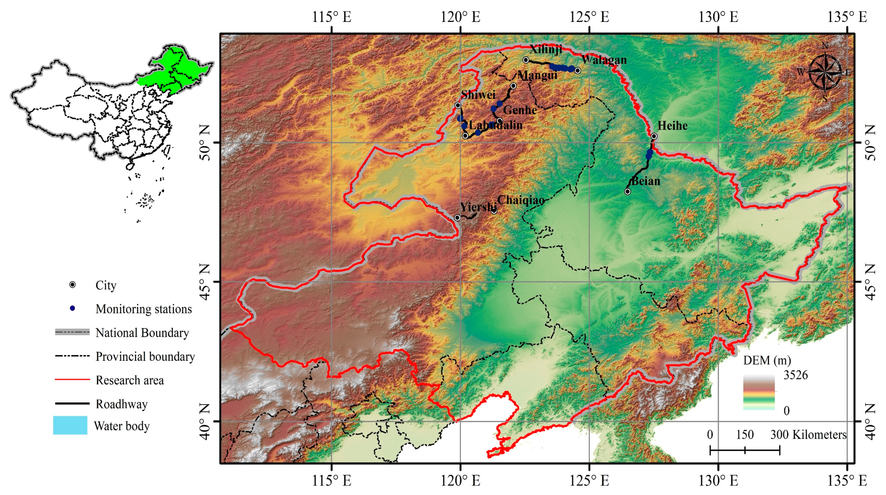
2.1. Study Region
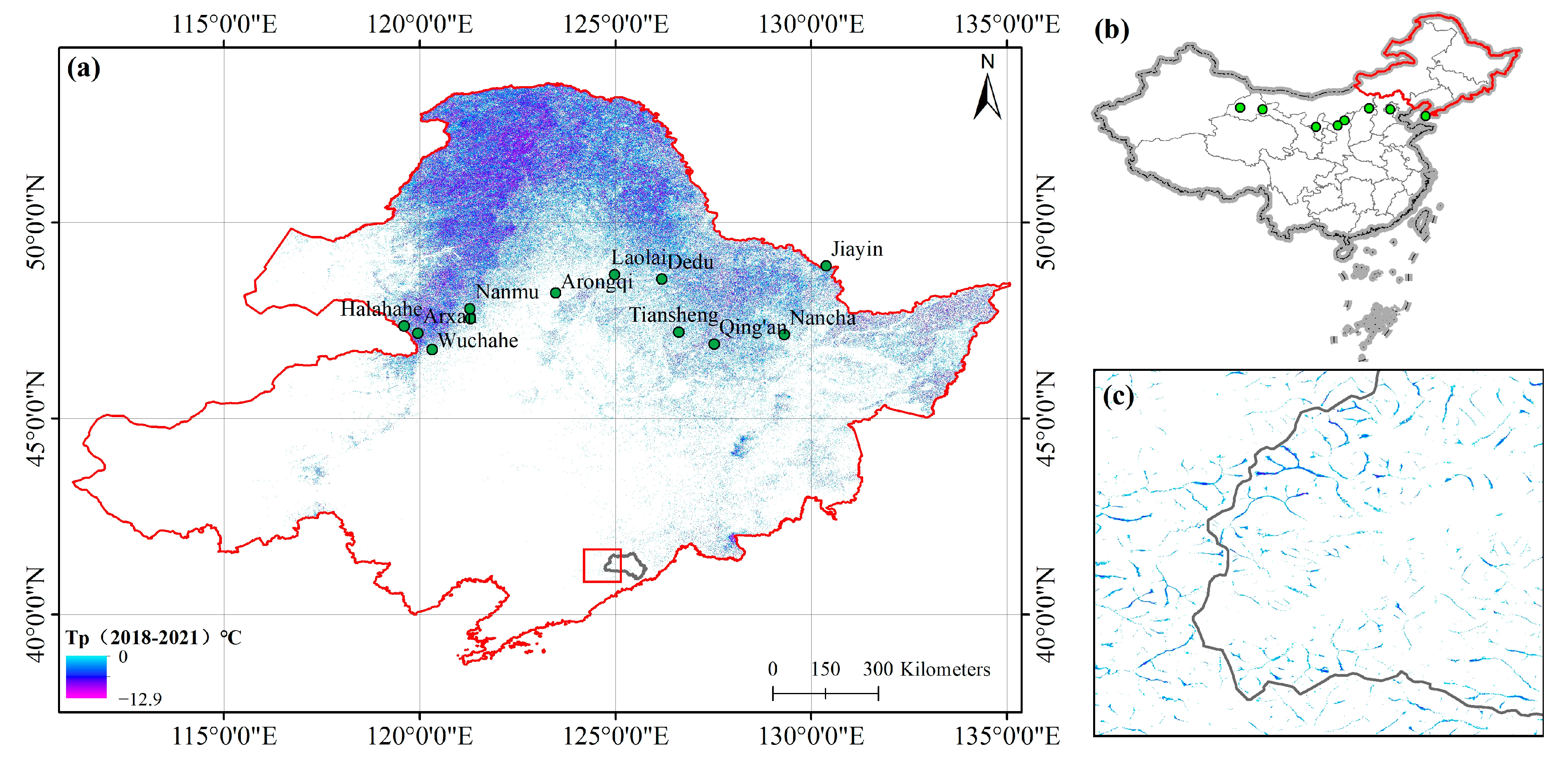
2.2. Monitoring Data
2.3. Surface Frost Number Model
2.4. Surface Frost Number Downscaling
2.5. Surface Frost Number and Permafrost Temperature
3. Results and Tests
3.1. Spatial Distribution and Variation Characteristics of Permafrost Temperature
3.2. Indirect Test
3.2.1. The Relative Accuracy of Permafrost Temperature
3.2.2. The Relative Accuracy of Permafrost Range
4. Discussion
4.1. Permafrost Area in Northeast China
4.2. Analysis of Permafrost Temperature Distribution
4.3. The Southern Boundary of Permafrost Region in the Northeast
4.4. Application Prospect of 30 m Resolution Permafrost Map
5. Conclusions
- During 2003–2007, 2008–2012, 2013–2017, and 2018–2021, the permafrost area is 28.35 × 10⁴ km2, 35.14 × 10⁴ km2, 28.96 × 10⁴ km2, and 25.21 × 10⁴ km2, respectively (excluding lakes).
- The proportion of permafrost of extremely stable, stable, sub-stable, transitional, and unstable types is 0.50~1.27%, 6.77~12.45%, 29.08~33.94%, 34.52~39.50%, and 19.87~26.79%, respectively. The permafrost area shows a decreasing trend, the temperature shows an increasing trend, and stability declines.
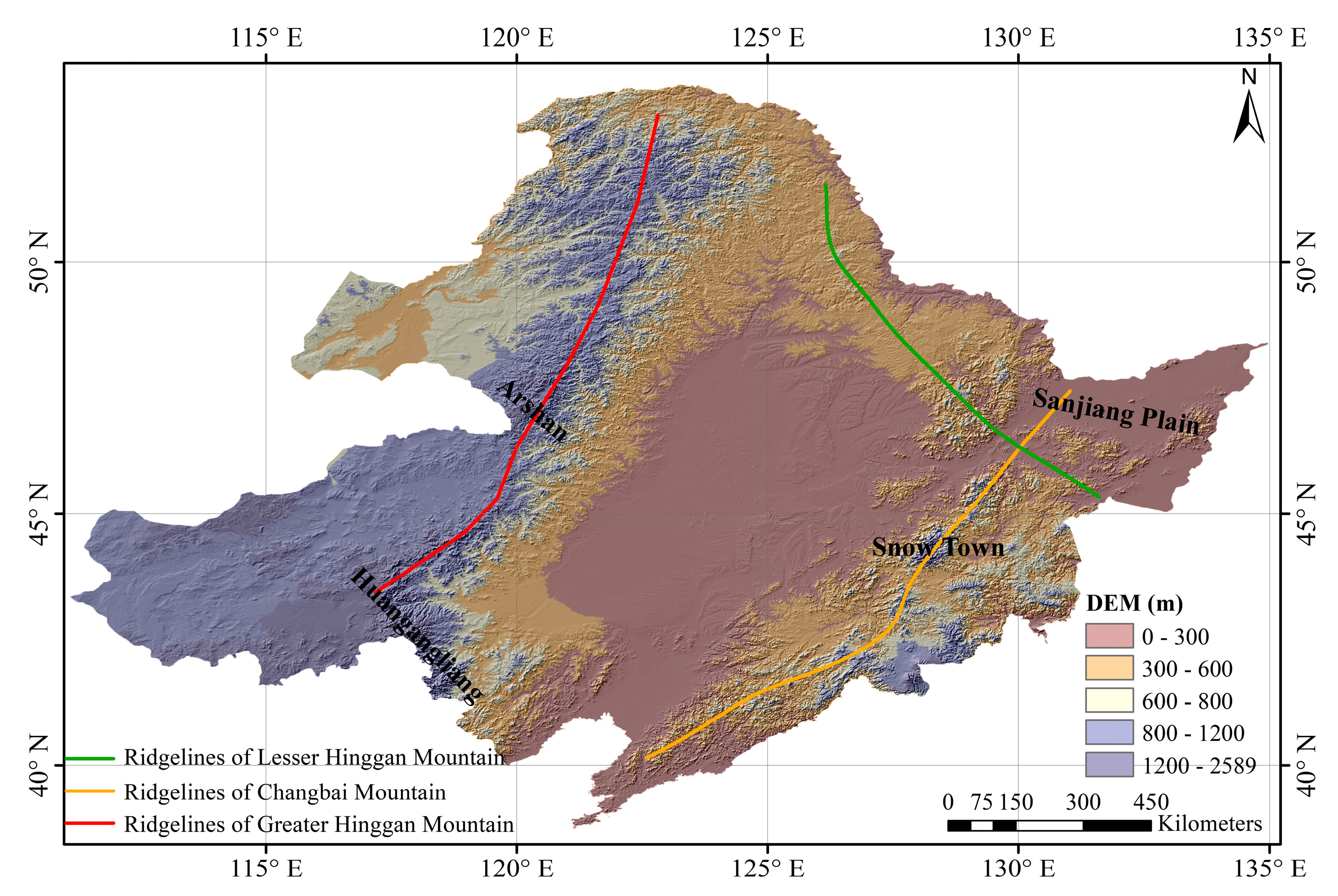
- The permafrost temperature in the Greater Khingan Mountain is mainly affected by elevation while the latitude has a more significant effect on the permafrost temperature in the Lesser Khingan Mountains and Changbai Mountain.
Author Contributions
Funding
Conflicts of Interest
References
- Li, X.; Cheng, G.; Jin, H.; Kang, E.; Che, T.; Jin, R.; Wu, L.; Nan, Z.; Wang, J.; Shen, Y. Cryospheric change in China. Glob. Planet. Chang. 2008, 62, 210–218. [Google Scholar] [CrossRef]
- Ran, Y.; Li, X.; Cheng, G.; Zhang, T.; Wu, Q.; Jin, H.; Jin, R. Distribution of permafrost in China: An overview of existing permafrost map. Permafr. Periglac. Process. 2012, 23, 322–333. [Google Scholar] [CrossRef]
- Yang, J.P.; Yang, S.Q.; Li, M.; Tan, C.P. Vulnerability of frozen ground to climate change in China. J. Glaciol. Geocryol. 2013, 35, 1436–1445. [Google Scholar]
- Peng, X.; Zhang, T.; Frauenfeld, O.W.; Wang, K.; Luo, D.; Cao, B.; Su, H.; Jin, H.; Wu, Q. Spatio-temporal changes in active layer thickness under contemporary and projected climate in the Northern Hemisphere. J. Clim. 2018, 31, 251–266. [Google Scholar] [CrossRef]
- Gubler, S.; Fiddes, J.; Keller, M.; Gruber, S. Scale-dependent measurement and analysis of ground surface temperature variability in alpine terrain. Cryosphere 2011, 5, 431–443. [Google Scholar] [CrossRef]
- Gubler, S.; Endrizzi, S.; Gruber, S.; Purves, R.S. Sensitivities and uncertainties of modeled ground temperatures in mountain environments. Geosci. Model. Dev. 2013, 6, 1319–1336. [Google Scholar] [CrossRef]
- Westermann, S.; Duguay, C.R.; Grosse, G.; Kääb, A. Remote sensing of permafrost and frozen ground. In Remote Sensing of the Cryosphere, 1st ed.; Tedesco, M., Ed.; Wiley-Blackwell: Chichester, UK, 2015; pp. 307–344. [Google Scholar]
- Jin, H.; Yu, S.; Lü, L.; Guo, D.; Li, Y. Degradation of the Da and Xiao Hinggan Mountains, Northeast China, and preliminary assessment of it’s trend. J. Glaciol. Geocryol. 2006, 28, 467–475. [Google Scholar]
- Zhou, Y.; Wang, Y.; Gao, X.; Yue, H. Ground Temperature, Permafrost Distribution and Climate Warming in Northeastern China. J. Glaciol. Geocryol. 1996, 20, 139–147. [Google Scholar]
- Nelson, F.E.; Outcalt, S.I. A Computational Method for Prediction and Regionalization of Permafrost. Arct. Alp. Res. 1987, 19, 279–288. [Google Scholar] [CrossRef]
- Nelson, F.E. Permafrost Distribution in Central Canada: Applications of a Climate-Based Predictive Model. Ann. Assoc. Am. Geogr. 1986, 76, 550–569. [Google Scholar] [CrossRef]
- Nelson, F.E.; Anisimov, O.A. Permafrost zonation in Russia under anthropogenic climatic change. Permafr. Periglac. Process. 1993, 4, 137–148. [Google Scholar] [CrossRef]
- Cao, B.; Zhang, T.; Peng, X.; Zheng, L.; Mu, C.; Wang, Q. Spatial Variability of Freezing-thawing Index over the Heihe River Basin. Adv. Earth Sci. 2015, 30, 357–366. [Google Scholar]
- Nan, Z.; LI, S.; Cheng, G.; Huang, P. Surface Frost Number Model and Its Application to the Tibetan Plateau. J. Glaciol. Geocryol. 2012, 34, 89–95. [Google Scholar]
- Hu, T.; Lü, S.; Chang, Y.; Yang, M.; Luo, J.; Cheng, X. Analysis and Prediction of Permafrost Changes in Qinghai-Xizang Plateau by CMIP6 Climate Models. Plateau Meteorol. 2022, 41, 363–375. [Google Scholar]
- Lv, J.; Li, X.; Hu, Y.; Wang, X.; Sun, J. Application of frost number model in Northeast China pepmafrost regionalization. Chin. J. Appl. Ecol. 2008, 10, 177–182. [Google Scholar]
- Zhang, Z.; Wu, Q.; Xun, X.; Wang, B.; Wang, X. Climate change and the distribution of frozen soil in 1980–2010 in northern northeast China. Quat. Int. 2018, 467 Pt B, 230–241. [Google Scholar] [CrossRef]
- Zhang, Z.; Wu, Q.; Xun, X.; Li, Y. Spatial distribution and changes of Xing’an permafrost in China over the past three decades. Quat. Int. 2019, 523, 16–24. [Google Scholar]
- Li, X. The Cryosphere Information System and Its Application. Ph.D. Thesis, Cold and Arid Regions Environmental and Engineering Reasearch Institute, Lanzhou, China, 1998. [Google Scholar]
- Wang, Z. Research on the Applications of Permafrost Distribution Models in the Qinghai-Tibet Plateau. Ph.D. Thesis, Lanzhou University, Lanzhou, China, 2010. [Google Scholar]
- Han, X. Dynamic response of Terrestrial ecosystem Carbon cycle to global climate change. J. Geosci. Transl. 1998, 15, 18–20. [Google Scholar]
- Jorgenson, M.T.; Romanovsky, V.; Harden, J.; Shur, Y.; O’Donnell, J.; Schuur, E.A.G.; Kanevskiy, M.; Marchenko, S. Resilience and vulnerability of permafrost to climate. Can. J. Res. 2010, 40, 1219–1236. [Google Scholar] [CrossRef]
- Woo, M.; Lewkowicz, A.G.; Rouse, W.R. Response of the Canadian permafrost environment to climatic change. Phys. Geogr. 1992, 13, 287–317. [Google Scholar] [CrossRef]
- Shan, W.; Zhang, C.; Guo, Y.; Qiu, L.; Xu, Z.; Wang, Y. Spatial Distribution and Variation Characteristics of Permafrost Temperature in Northeast China. Sustainability 2022, 14, 8178. [Google Scholar] [CrossRef]
- Shan, W.; Zhang, C.; Guo, Y.; Qiu, L. Mapping the Thermal State of Permafrost in Northeast China Based on the Surface Frost Number Model. Remote Sens. 2022, 14, 3185. [Google Scholar] [CrossRef]
- Zhou, Y.W.; Guo, D.X.; Qiu, G.Q. China Permafrost; Science Press: Beijing, Chian, 2000. [Google Scholar]
- Guo, D.; Wang, S.; Lu, G.; Dan, J. Division of permafrost regions in Daxiao Hinggan Ling northeast China. J. Glaciol. Geocryol. 1981, 3, 1–9. [Google Scholar]
- Jin, H.; Yu, Q.; Lü, L.; Guo, D.; He, R.; Yu, S.; Sun, G.; Li, Y. Degradation of permafrost in the Xing’anling Mountains, northeastern China. Permafr. Periglac. Process. 2007, 18, 245–258. [Google Scholar] [CrossRef]
- Dai, J. Characteristics of ground temperature in permafrost areas in the northern part of great xinan mountain. J. Glaciol. Geocryol. 1982, 4, 53–63. [Google Scholar]
- Obu, J.; Westermann, S.; Bartsch, A.; Berdnikov, N.; Christiansen, H.H.; Dashtseren, A.; Delaloye, R.; Elberling, B.; Etzelmüller, B.; Kholodov, A.; et al. Northern Hemisphere permafrost map based on TTOP modelling for 2000–2016 at 1 km2 scale. Earth Sci. Rev. 2019, 193, 299–316. [Google Scholar] [CrossRef]
- Gruber, S. Derivation and analysis of a high-resolution estimate of global permafrost zonation. Cryosphere 2012, 6, 221–233. [Google Scholar] [CrossRef]
- Zou, D.F.; Zhao, L.; Sheng, Y.; Chen, J.; Hu, G.; Wu, T.; Wu, J.; Xie, C.; Wu, X.; Pang, Q. A new map of permafrost distribution on the Tibetan Plateau. Cryosphere 2017, 11, 2527–2542. [Google Scholar] [CrossRef]
- Ran, Y.; Li, X.; Jin, R.; Guo, J. Remote sensing of the mean annual surface temperature and surface frost number for mapping permafrost in China. Arct. Antarct. Alp. Res. 2015, 47, 255–265. [Google Scholar] [CrossRef]
- Doblas-Reyes, F.J.; Srensson, A.A.; Almazroui, M.; Dosio, A.; Gutowski, W.J.; Haarsma, R.; Hamdi, R.; Hewitson, B.; Kwon, B.T.; Lamptey, B.L.; et al. IPCC AR6 WGI Chapter 10: Linking global to regional climate change. In Climate Change 2021: The Physical Science Basis; Masson-Delmotte, V.P., Zhai, A., Pirani, S.L., Connors, C., Péan, S., Berger, N., Caud, Y., Chen, L., Goldfarb, M.I., Gomis, M., et al., Eds.; Cambridge University Press: Cambridge, UK; New York, NY, USA, 2021; pp. 1363–1512. [Google Scholar]
- Solomon, S.D.; Qin, D.; Manning, M.; Chen, Z.; Miller, H.L. Climate Change 2007: The Physical Science Basis. Working Group I Contribution to the Fourth Assessment Report of the IPCC; Intergovernmental Panel on Climate Change Climate Change: Geneva, Switzerland, 2007. [Google Scholar]
- Shan, W.; Xu, Z.; Guo, Y.; Zhang, C.; Zhao, H.; Wang, Y. Geological methane emissions and wildfire risk in the degraded permafrost area of the Xiao Xing’an Mountains, China. Sci. Rep. 2020, 10, 21297. [Google Scholar] [CrossRef]
- Xiao, C.D.; Wang, S.J.; Qin, D.H. A preliminary study of cryosphere service function and value evaluation. Adv. Clim. Chang. Res. 2015, 6, 181–187. [Google Scholar] [CrossRef]
- Guo, Y.; Shan, W.; Zhang, C.; Hu, Z.; Wang, S.; Gao, J. Monitoring of permafrost degradation along the Bei’an-Heihe Expressway in China. Bull. Eng. Geol. Environ. 2020, 16, 1–10. [Google Scholar] [CrossRef]
- Ma, J.; Li, R.; Liu, H.; Wu, T.; Xiao, Y.; Du, Y.; Yang, S.; Shi, J.; Qiao, Y. A review on the development of study on hydrothermal characteristics of active layer in permafrost areas in Qinghai-Tibet Plateau. J. Glaciol. Geocryol. 2020, 42, 195–204. [Google Scholar]
- Yang, S.; Li, R.; Wu, T.; Hu, G.; Xiao, Y.; Du, Y.; Zhu, X.; Ni, J. The variation characteristics of different freeze-thaw status in the near surface and the relationship with temperature over the Qinghai-Tibet Plateau. J. Glaciol. Geocryol. 2019, 41, 1377–1387. [Google Scholar]
- Yang, C.; Wu, T.; Yao, J.; Li, R.; Xie, C.; Hu, G.; Zhu, X.; Hao, j.; Ni, J.; Li, X. Temporal and Spatial Characteristics of Ground Surface Soil Heat Flux over the Qinghai-Ti-betan Plateau. Plateau Meteorol. 2020, 39, 706–718. [Google Scholar] [CrossRef]
- Qin, Y.; Wu, T.; Li, R.; Hu, G.; Qiao, Y.; Zhu, X.; Yang, S.; Yu, W.; Wang, W. Thermal condition of the active layer on the Qinghai-Tibet Plateau simulated by using the Model of GIPL2. J. Glaciol. Geocryol. 2018, 40, 1153–1166. [Google Scholar]
- Wang, C.; Shan, W.; Guo, Y.; Hu, Z.; Jiang, H. Permafrost Distribution Study Based on Landsat ETM+ Imagery of the Northwest Section of the Lesser Khingan Range, China. In Landslide Science for a Safer Geoenvironment; Sassa, K., Canuti, P., Yin, Y., Eds.; Springer International Publishing: Berlin, Germany, 2014; Volume 3, pp. 529–534. [Google Scholar]
- Wei, S.; Hua, J.; Hu, Z.; Guo, Y.; Wang, C. Island Permafrost Degrading Process and Deformation Characteristics of Expressway Widen Subgrade Foundation. Disaster Adv. 2012, 5, 827–832. [Google Scholar]
- Yang, Y.; Cheng, D.; Fu, H. Engineering geological characteristics and evaluations of permafrost in Daxing’an mountains. J. Eng. Geol. 2008, 16, 657–662. [Google Scholar]
- Wang, C.; Shan, W.; Guo, Y.; Hu, Z.; Jiang, H. Relative factors of Beihei Highway’s ground deformation interpretation based on remote-sensing imagery technology. In Landslides in Cold Regions in the Context of Climate Change; Wei, S., Guo, Y., Wang, F., Marui, H., Strom, A., Eds.; Springer International Publishing: Berlin, Germany, 2014; pp. 191–204. [Google Scholar]
- Fensholt, R.; Rasmussen, K.; Nielsen, T.T.; Mbow, C. Evaluation of earth observation based long term vegetation trends-Intercomparing NDVI time series trend analysis consistency of Sahel from AVHRR GIMMS, Terra MODIS and SPOT VGT data. Remote Sens. Environ. 2009, 113, 1886–1898. [Google Scholar] [CrossRef]
- Poutou, E.; Krinner, G.; Genthon, C. Role of soil freezing in future boreal climate change. Clim. Dyn. 2004, 23, 621–639. [Google Scholar] [CrossRef]
- Guo, J.; Hu, Y.; Xiong, Z.; Yan, X.; Bu, R. Spatiotemporal variations of growing-season NDVI and response to climate change in permafrost zone of Northeast China. Chin. J. Appl. Ecol. 2017, 28, 2413–2422. [Google Scholar]
- Chang, X.; Jin, H.; Wang, Y.; Zhang, Y.; Zhou, G.; Che, F.; Zhao, Y. Influences of vegetation on permafrost: A review. Acta Ecol. Sin. 2012, 32, 7981–7990. [Google Scholar] [CrossRef]
- Liu, Y.; Hu, Z.; Jiang, H.; Shan, W. Application of High-density Resistance to Detect Island Permafrost Distribution under the Foundation in High-latitude Frozen Regions. For. Eng. 2014, 30, 161–165. [Google Scholar] [CrossRef]
- Liu, F.; Lv, Y.; Jiang, L.; Xin, H.; Zhang, T.; Lv, X. Correlation Analysis between Modis Brightness Temperature and Surface Temperature Provided by Meteorological Station. Seismol. Geol. 2010, 32, 127–137. [Google Scholar]
- Ke, L.; Wang, Z.; Song, C.; Lu, Z. Reconstruction of MODIS LST Time Series and Comparison with Land Surface Temperature (T) among Observation Stations in the Northeast Qinghai-Tibet Plateau. Prog. Geogr. 2011, 30, 819–826. [Google Scholar]
- Li, M.; Guo, H.; Fan, W.; Zhen, Z. Remote Sensing Analysis of Forest Site Quality in Daxing’an Mountain Based on GWR. Sci. Silvae Sin. 2017, 6, 59–69. [Google Scholar]
- Wei, H.; Dong, L.; Liu, Z. Spatial structure optimization simulation of main forest types in Great Xing’an Mountains, Northeast China. Chin. J. Appl. Ecol. 2019, 30, 3824–3832. [Google Scholar]
- Zhao, L.; Sheng, Y.; Nan, Z.; Wu, T.; Zhou, G. Permafrost Survey Manual; Ke Xue Chu Ban She Press: Beijing, China, 2015. [Google Scholar]
- Harris, S.A.; Brouchkov, A.; Guodong, C. Geocryology: Characteristics and Use of Frozen Ground and Permafrost Landforms; CRC Press: Boca Raton, FL, USA, 2017. [Google Scholar]
- Amici, V. Dealing with vagueness in complex forest landscapes: A soft classification approach through a niche-based distribution model. Ecol. Inform. 2011, 6, 371–383. [Google Scholar] [CrossRef]
- Fu, P. A Geometric Solar Radiation Model with Applications in Landscape Ecology. Ph.D. Thesis, Department of Geography, University of Kansas, Lawrence, KS, USA, 2000. [Google Scholar]
- Fu, P.; Rich, P.M. A geometric solar radiation model with applications in agriculture and forestry. Comput. Electron. Agric. 2002, 37, 25–35. [Google Scholar] [CrossRef]
- Wilson, J.P.; Gallant, J.C. Digital Terrain Analysis in Terrain Analysis: Principles and Applications. In Terrain Analysis: Principles and Applications; Gallant, J.C., Ed.; John Wilson John Wiley & Sons. Press: New York, NY, USA, 2000; pp. 1–27. [Google Scholar]
- Weiss, A. Topographic position and landforms analysis. In Proceedings of the Poster Presentation, ESRI User Conference, San Diego, CA, USA, 9–13 July 2001; Volume 200. [Google Scholar]
- De Reu, J.; Bourgeois, J.; Bats, M.; Zwertvaegher, A.; Gelorini, V.; De Smedt, P.; Chu, W.; Antrop, M.; De Maeyer, P.; Finke, P. Application of the topographic position index to heterogeneous landscapes. Geomorphology 2013, 186, 39–49. [Google Scholar] [CrossRef]
- Theobald, D.M.; Harrison-Atlas, D.; Monahan, W.B.; Albano, C.M. Ecologically-relevant maps of landforms and physiographic diversity for climate adaptation planning. PLoS ONE 2015, 10, e0143619. [Google Scholar] [CrossRef] [PubMed]
- Cheng, G. Problems On Zonation Of High-Altitude Permafrost. Acta Geogr. Sin. 1984, 39, 185–193. [Google Scholar]
- Editor Committee of Local Records in Heilongjiang Province. Heilongjiang Records‚ 4:Geological-Mineral Records; People Press of Heilongjiang Province: Harbin, China, 1994; pp. 185–193. [Google Scholar]
- Wang, C.; Shan, M.; Hu, Z.; Shan, W. Multi-spectral remote sensing based land surface temperature retrieval and isolated permafrost zone segmentation. Infrared Laser Eng. 2015, 44, 1390–1396. [Google Scholar]
- Ran, Y.; Li, X. Progress, Challenges and opportunities of permafrost mapping in China. Adv. Earth Sci. 2019, 34, 1015–1027. [Google Scholar] [CrossRef]
- Xin, K.; Ren, Q. Distribution of permafrost in Northeast China. Geol. China 1956, 10, 15–18. [Google Scholar]
- Shi, Y.; Mi, D. Distribution Map of Frozen Ground in China Based on Map of Snow, Ice and Frozen Ground in China (1998); National Tibetan Plateau Data Center: Beijing, China, 2013. [Google Scholar]
- Zhou, Y.W.; Guo, D.X.; Qiu, G.Q. Geocryological Regionalization and Classification Map of the Frozen Soil in China (1:10,000,000); National Tibetan Plateau Data Center: Beijing, China, 2000. [Google Scholar]
- Nan, Z.; Li, S.; Liu, Y. Mean Annual Ground Temperature Distribution on the Tibetan Plateau: Permafrost Distribution Mapping and Further Application. J. Glaciolgy Geocryol. 2002, 2, 142–148. [Google Scholar]
- Wang, T.; Shi, Y.; Guo, D. Frozen Ground Map of China Based on a Map of the Glaciers, Frozen Ground and Deserts in China (1981–2006); National Tibetan Plateau Data Center: Beijing, China, 2012. [Google Scholar]
- Wei, Z.; Jin, H.; Zhang, J.; Yu, S.; Han, X.; Ji, Y.; He, R.; Chang, X. Prediction of permafrost changes in Northeastern China under a changing climate. China Earth Sci. 2011, 54, 924–935. [Google Scholar] [CrossRef]
- Zhang, Z.Q.; Wu, Q.B.; Hou, M.T.; Tai, B.W.; AN, Y.K. Permafrost change in Northeast China in the 1950–2010s. Adv. Clim. Chang. Res. 2021, 12, 18–28. [Google Scholar] [CrossRef]
- Wang, Y.; Tan, D.; Han, L.; Li, D.; Wang, X.; Lu, G.; Lin, J. Review of climate change in the Yellow River Basin. Rev. Clim. Chang. Yellow River Basin 2021, 41, 235–246. [Google Scholar]
- Zhang, T. Progress in global permafrost and climate change studies. Quat. Sci. 2012, 32, 27–38. [Google Scholar]
- Cui, Z.; Yang, J.; Zhao, L.; Zhang, W.; Xie, Y. The Discovery of a Large Area Ice Wedge Group in Ordos and the Southern Boundary and Environment of Permafrost in Northern China Since 20 ka. Chin. Sci. Bull. 2004, 49, 1304–1310. [Google Scholar] [CrossRef]
- Zhao, W.; Liu, D. The analysis and prevention of Ji-Yan highway salivary flow ice. J. Chang. Inst. Technol. (Soc. Sci. Ed.) 2012, 13, 7–9. [Google Scholar]
- Yu, N. Brief analysis on salivary flow ice treatment measure of HEDA expressway Huanren (Xinkailing) to Dandong (Guchengzi) section. North. Commun. 2013, 5–8. [Google Scholar] [CrossRef]
- Lu, G.; Weng, B.; Guo, D. The Geographic Boundary of Permafrost in the Northeast of China. J. Glaciol. Geocryol. 1993, 15, 214–218. [Google Scholar]
- Webb, E.E.; Liljedahl, A.K.; Cordeiro, J.A.; Loranty, M.M.; Witharana, C.; Lichstein, J.W. Permafrost thaw drives surface water decline across lake-rich regions of the Arctic. Nat. Clim. Change 2022, 12, 841–846. [Google Scholar] [CrossRef]
- Chang, K.Y.; Riley, W.J.; Crill, P.M.; Grant, R.F.; Rich, V.I.; Saleska, S.R. Large carbon cycle sensitivities to climate across a permafrost thaw gradient in subarctic Sweden. Cryosphere Discuss. 2019, 13, 647–663. [Google Scholar] [CrossRef]
- Jie, N.; Tonghua, W.; Lin, Z. Carbon cycle in circum-Arctic permafrost regions: Progress and prospects. J. Glaciol. Geocryol. 2019, 41, 101–113. [Google Scholar]
- Jingyun, F.; Songlin, F. Carbon cycle in the Arctic terrestrial ecosystems in relation to the global warming. Chin. J. Polar Sci. 1998, 9, 92–100. [Google Scholar]
- Shan, W.; Qiu, L.; Guo, Y.; Zhang, C.; Xu, Z.; Liu, S. Spatiotemporal Distribution Characteristics of Fire Scars Further Prove the Correlation between Permafrost Swamp Wildfires and Methane Geological Emissions. Sustainability 2022, 14, 14947. [Google Scholar] [CrossRef]
- Baltzer, J.L.; Day, N.J.; Walker, X.J.; Johnstone, J.F. Increasing fire and the decline of fire adapted black spruce in the boreal forest. Proc. Natl. Acad. Sci. USA 2021, 118, e2024872118. [Google Scholar] [CrossRef]
- Li, X.; Jin, H.; Wang, H.; Marchenko, S.S.; Jia, N. Influences of forest fires on the permafrost environment: A review. Adv. Clim. Chang. Res. 2021, 12, 48–65. [Google Scholar] [CrossRef]


| Permafrost Stability Types | Extremely Stable | Stable | Sub-Stable | Transitional | Unstable | Area (×104 km2) | Minimum Tp (°C) | Mean Annual Air Temperature (°C) |
|---|---|---|---|---|---|---|---|---|
| 2003–2007 | 0.27 | 2.90 | 9.25 | 10.14 | 5.79 | 28.35 | −13.3 | 3.2 |
| 2008–2012 | 0.45 | 4.37 | 11.93 | 12.13 | 6.98 | 35.14 | −13.9 | 2.6 |
| 2013–2017 | 0.18 | 2.34 | 8.98 | 10.94 | 7.76 | 28.96 | −13.1 | 3.1 |
| 2018–2021 | 0.13 | 1.71 | 7.33 | 9.96 | 6.09 | 25.21 | −12.9 | 4.0 |
| No. | Location | Road Length (km) | Number of Boreholes | Drilling Depth (m) | Permafrost Section Length (km) | Drilling Time | Same Length as Investigation Data | Consistency |
|---|---|---|---|---|---|---|---|---|
| 1 | Walagan–Xilinji section of National Highway G111 | 157.01 | 1112 | 3.5~40 | 47.26 | September. 2017 | 45.59 | 96.47% |
| 2 | Genhe–Mangui section of provincial highway S204 | 255.00 | 522 | 5~40 | 112.98 | May. 2020 | 108.04 | 95.63% |
| 3 | Jiageda–Changqing Forest Farm section of National Highway G331 | 52.85 | 161 | 5~25 | 11.52 | May. 2020 | 10.16 | 88.19% |
| 4 | Kubuchun Forest Farm–Genhe section of National Highway G332 | 59.69 | 382 | 5~35 | 34.58 | December. 2020 | 30.23 | 87.74% |
| 5 | Shiwei–Labudalin Highway section of National Highway G331 | 153.74 | 425 | 5~40 | 29.01 | July. 2012 | 24.14 | 83.21% |
| 6 | Yiershi–Chaiqiao section of provincial highway S308 | 87.08 | 243 | 5~40 | 5.35 | July. 2017 | 4.45 | 83.17% |
| Permafrost Map Name | Area (104 km2) | Age | Source |
|---|---|---|---|
| Distribution of permafrost in Northeast China | 40~50 | 1950s | Xin KuiDe, Ren QiJia [69], 1956 |
| Division of permafrost regions in Daxiao Hinggan Ling Northeast China (1:200,000) | 38.67 | 1970s | Guo Dongxin, et al. [27], 1981 |
| Map of snow, ice, and frozen ground in China (1:400,000) | 38–39 | 1990s | Shi Yafeng, Mi Desheng [70], 1988 |
| Geocryological regionalization and classification map of the frozen soil in China (1:1000,000) | 39 | 1990s | Zhou Youwu, et al. [71], 2000 |
| Map of the Glaciers, Frozen Ground and Deserts in China (1:400,000) | 39 | 1980–1990s | Nan zhuotong, et al. [72], 2002; Wang Tao [73], 2006 |
| Frozen soil map of China | 24.0 | 2000s | Ran Youhua, Li Xin [2] (2018) |
| No Name | 25.7 | 2000s | Wei Zhi, et al. [74] |
| No Name | 27.10 | 2003–2019 | Shan, et al. [24] |
Disclaimer/Publisher’s Note: The statements, opinions and data contained in all publications are solely those of the individual author(s) and contributor(s) and not of MDPI and/or the editor(s). MDPI and/or the editor(s) disclaim responsibility for any injury to people or property resulting from any ideas, methods, instructions or products referred to in the content. |
© 2023 by the authors. Licensee MDPI, Basel, Switzerland. This article is an open access article distributed under the terms and conditions of the Creative Commons Attribution (CC BY) license (https://creativecommons.org/licenses/by/4.0/).
Share and Cite
Zhang, C.; Shan, W.; Liu, S.; Guo, Y.; Qiu, L. Simulation of Spatiotemporal Distribution and Variation of 30 m Resolution Permafrost in Northeast China from 2003 to 2021. Sustainability 2023, 15, 14610. https://doi.org/10.3390/su151914610
Zhang C, Shan W, Liu S, Guo Y, Qiu L. Simulation of Spatiotemporal Distribution and Variation of 30 m Resolution Permafrost in Northeast China from 2003 to 2021. Sustainability. 2023; 15(19):14610. https://doi.org/10.3390/su151914610
Chicago/Turabian StyleZhang, Chengcheng, Wei Shan, Shuai Liu, Ying Guo, and Lisha Qiu. 2023. "Simulation of Spatiotemporal Distribution and Variation of 30 m Resolution Permafrost in Northeast China from 2003 to 2021" Sustainability 15, no. 19: 14610. https://doi.org/10.3390/su151914610
APA StyleZhang, C., Shan, W., Liu, S., Guo, Y., & Qiu, L. (2023). Simulation of Spatiotemporal Distribution and Variation of 30 m Resolution Permafrost in Northeast China from 2003 to 2021. Sustainability, 15(19), 14610. https://doi.org/10.3390/su151914610