Abstract
While the efficiency of incorporating phenology features into vegetation type classification, in general, and coastal wetland vegetation classification, in particular, has been verified, it is difficult to acquire high-spatial-resolution (HSR) images taken at appropriate times for vegetation identification using phenology features because of the coastal climate and the HSR satellite imaging cycle. To strengthen phenology feature differences, in this study, we constructed vegetation phenology metrics according to vegetation NDVI time series curves fitted by samples collected from the Linhong Estuary Wetland and Liezi Estuary Wetland based on Gao Fen (GF) series satellite images taken between 2018 and 2022. Next, we calculated the phenology metrics using GF series satellite imagery taken over the most recent complete phenology cycle: 21 October 2020, 9 January 2021, 19 February 2021, and 8 May 2021. Five vegetation type classifications in the Linhong Estuary Wetland were carried out using single images of 21 October 2020 and 8 May 2021, along with their combination and the further addition of phenology metrics. From our comparison and analysis, the following findings emerged: Combining the images taken in 21 October 2020 and 8 May 2021 provided better vegetation classification accuracy than any single image, and the overall accuracy was, respectively, increased from 47% and 48% to 67%, while the corresponding kappa was increased from 33% and 34% to 58%; however, adding phenology metrics further improved the accuracy by decreasing the effect of some confusion among different vegetation types, and the overall accuracy and kappa were further improved to 75% and 69%, respectively. Though some problems remain to be further dealt with, this exploration offers helpful insights into coastal wetland vegetation classification using phenology based on HSR imagery.
1. Introduction
Vegetation phenology involves the timing of seasonal developmental stages in plant life cycles, including bud burst, canopy growth, flowering, and senescence [1,2]. Phenology events are very useful for vegetation type classification, especially for coastal wetland vegetation, because phenology features are very efficient for dealing with similar spectral characteristics of the vegetation types [3]. To describe vegetation phenology events, high-resolution temporal images are necessary. Therefore, satellite images exhibit advantages for this task, because of their characteristics of high temporal resolution, fine accessibility, and multi-spectral bands.
Coarse-spatial-resolution images (≥30 m)—for example, the Moderate-Resolution Imaging Spectroradiometer (MODIS) [4] or the Advanced Very High-Resolution Radiometer (AVHRR) [5]—have contributed to obtaining image vegetation index (VI) time series and constructing a phenology fitting curve through various fitting functions [6]. However, by these coarse-spatial-resolution images, phenology parameters generally tend to describe the aggregate temporal behavior of multiple plant species at a large scale, and individual plants cannot be classified except in the case of a homogeneous landscape pattern [7,8,9,10,11]. Moderate-spatial-resolution remote sensing imagery (≤30 m), such as that provided by Landsat or Sentinel-2 satellites, allows a phenology time series to be derived at the landscape scale [8,12,13]. In addition, the scope of phenology explored can be extended into areas of mixed vegetation and forest stands [14].
However, the temporal resolution of these images is much lower than that found in MODIS or AVHRR data and offers challenges to extracting phenology metrics due to the influence of clouds and shadows. Several approaches have been developed to deal with this challenge when retrieving phenology parameters, including (1) combining multi-sensor or multiple-year images and (2) pixel-based compositing [8,15,16,17,18,19,20]. This image processing increases the temporal resolution of cloud-free image data that can be used for phenology description. Next, phenology features are retrieved and employed to carry out vegetation type classification, primarily using one of the following two approaches: spectral-temporal metrics (STM) and temporal time series [21,22,23,24]. The STM method entails computing statistics related to the characteristics revealed in the cloud-free observations, including the mean, minimum, maximum, standard deviation, and range for classification performance. In contrast, the time series technique involves calculating phenology metrics, such as start of growing season, peak of growing season, and end of growing season, to use as classification features [3].
The efficiency of these approaches has been verified for coastal wetland vegetation classification when using time series images from Landsat, Sentinel, or other similar satellite platforms to map Spartina alterniflora Loisel (S. alterniflora) [19,25] or to classify coastal wetland plant species [26]. Nevertheless, due to limitations imposed by a low revisit cycle and high costs, the studies about phenology metrics based on HSR images are still limited [27,28,29,30]. Phenology application studies for HSR images for vegetation classification have focused on the combinations of images taken in different seasons, according to the knowledge of evergreen and deciduous plants [31,32,33,34,35,36].
Now, for Lianyungang estuarine wetlands, vegetation type classification using the HSR remote sensing technique has become essential for coastal wetland protection [37], because this area plays an important role for birds inhabiting [38,39], while its vegetation pattern is heterogeneous and fragmented due to invasive vegetation and human activity [40,41]. The advent of Chinese GaoFen (GF) Series Satellites that provide three kinds of HSR images (GF-1, GF-2, and GF-6) has increased the accessibility of HSR images, providing a greater opportunity to explore the time series of different variations in vegetation phenology [42,43,44]. With these images, although we cannot precisely acquire key phenology times by images’ time series, it is practical to calculate phenology metrics using optimized time windows decided by vegetation phenology phases for vegetation classification improvement. Aimed at this objective, this study was carried out as follows: (1) to decide the optimized windows using GF images’ NDVI time series curves fitted by vegetation samples collected from both Linhong Estuary Wetland and Liezi estuary wetland within four years; (2) to construct phenology metrics according to the optimized windows and vegetation phenology events; (3) to perform vegetation type classification using a random forest (RF) method based on object-oriented technology, as well as to verify the efficiency of phenology metrics for improving the accuracy of vegetation classification. Constructed phenology metrics improve estuarine wetland vegetation type classification and provide an efficient method for fully utilizing GF images for estuarine wetland ecological system protection and monitoring.
2. Materials and Methods
2.1. Study Area
Two coastal wetlands in Lianyungang, Jiangsu province, China, were selected as the study area, including the Linhong Estuary Wetland and Liezi Estuary Wetland. The Linhong Estuary Wetland (119°11′37″–119°16′33″ E, 34°45′37″–34°49′15″ N) is located in the northern part of the Lianyungang coastal zone, while the Liezi Estuary Wetland (119°35′24″–119°44′54″ E, 34°28′37″–34°33′15″ N) is located in the southern part of Lianyungang. The distance between these two areas is about 49 km, and their coverage is about 102 km2 and 64 km2, respectively (Figure 1). Of the two areas, the Linhong Estuary Wetland was the main study site in which most of the samples used in the time series construction were surveyed and vegetation type classification was carried out. In contrast, for the Liezi Estuary Wetland, only four scene images from a recent four-year period (2018–2021) were acquired and used to provide samples for time series construction. All data used in this study are shown in Table 1.
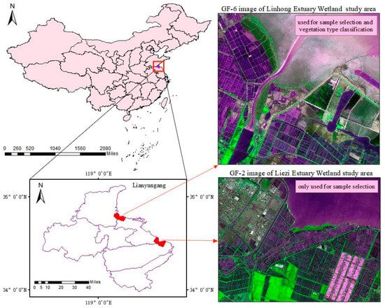
Figure 1.
The location of study sites on the coast of Lianyungang, Jiangsu Province, in northeast China.

Table 1.
The data used in this study and their parameters.
The Lianyungang coastal zone, which is characterized by flat topography with a warm, temperate, humid monsoon climate, is the key stopover and wintering site for shorebirds on the East Asian-Australasian Flyway [38,45,46]. The study area features three main vegetation species, including Spartina alterniflora Loisel (S. alterniflora), Phragmites australias (Cav.) Trin. ex Steud. (P. australis), and Suaeda salsa (Linn.) Pall. (S. salsa) [25,26,47,48]. In particular, S. alterniflora is an invasive vegetation species that is mainly located along two sides of the estuary subject to cyclical tidal flooding. In contrast, P. australis and S. salsa are dominant native vegetation species. Of the two, P. australis has a strong root system and has spread out to dominate large areas along two sides of the Linhong Estuary wetland, while S. salsa is a type of native pioneer plant that can grow in dry, high-salt conditions. S. salsa is vulnerable to invasion by S. alterniflora on wet land and P. australis on dry land, making its dispersion fragmented and changeable. In addition to these three species, other vegetation types are Road green space (R. green space) and M. weeds. R. green space is constructed according to human design and often comprises evergreen and deciduous vegetation. Mixed weeds (M. weeds) is usually found on temporarily vacant land formed by infill-up engineering and is often mixed with P. australis or S. salsa.
2.2. Data and Pre-Processing
All data were acquired from the following website by Lianyungang Natural Resources and Planning Bureau: http://www.sasclouds.com/chinese/normal/ (accessed on 26 April 2022). Three kinds of GF series satellite images (GF-1, GF-2, and GF-6) were selected to construct the full phenology cycle time series for each vegetation type. The selected images, taken during a four-year period (2018–2021), were carefully verified to ensure that all images were cloud-free and no tidal fluctuation had affected the vegetation within the study area. Table 1 displays detailed information about the four multi-spectral bands and one panchromatic band contained in each image. However, the data used for vegetation classification were imaged between 2020 and 2021 to reduce the influence of land-use changes on the classification results. All images used in this study can be seen in Table 1.
The Fast Line-of-sight Atmospheric Analysis of Spectral Hypercubes (FLAASH) model was employed to perform atmospheric correction for all multi-spectral data. In addition, a 3D polynomial model was applied to conduct geometric correction for both panchromatic and multi-spectral data. The control points used for geometric correction were selected on a 0.3 m aerial ortho-rectification image. All the above procedures were carried out using ENVI 5.6 processing image software.
Based on the processing described above, multi-spectral and pan images were fused via the Gram–Schmidt algorithm, which uses multi-spectral images to simulate panchromatic images that can effectively retain image spectral information and high-fidelity characteristics [49]. In this study, the normalized difference vegetation index (NDVI) calculated by the fused images using ENVI 5.6 software was employed to construct the phenology time series and perform image classification. To verify the consistency of NDVI values calculated by the fused image and multi-spectral image, we compared the vegetation sample mean and deviation by random selection on four scene images; the results illustrated that the values of the NDVI data calculated by fused and multi-spectral were very consistent and were closely related.
2.3. Method
2.3.1. Vegetation Types and Sampling
The field surveying for samples used in this study were mainly carried out during the period of 2018 to 2021, with the help of Lianyungang City Forestry Technology Guidance Station. As the government department management, they have definite practical requirements for coastal wetland vegetation classification when using the remote sensing technique. For a long time, they have continued to carry out field surveying and are familiar with vegetation composition and spatial distribution in the study area.
During the process of investigating, the position location of vegetation samples was finished by the GNSS system. However, limited by the accessibility of coastal wetland, some of the field investigating work could only be carried out along the roadside. In this case, samples can be plotted by visual interpretation depending on the spatial structure and spectral information of various objects that have been already fully expressed on HSR images, such as the road intersection, turning point of water, and corner of buildings. To enable each sample region to correspond to the marked type, the delineation was carried out within larger vegetation patches.
The selected samples for time series construction should be identified one by one on each image to ensure that it did not change from 2018 to 2021, especially for R. green space and M. weeds, which maintains the status of changing induced by human disturbance. There are 1300 samples in Linhong Estuary: 296 of S. alterniflora, 478 of P. australis, 162 of S. salsa, 193 of R. green space, and 171 of M. weeds; 200 samples in Liezi Estuary, 65 of S. alterniflora, 89 of P. australis, 5 of S. salsa, 31 of R. green space, and 10 of M. weeds. All the samples that did not change in the two areas were used to construct the vegetation time series, while for the image classification, 1300 samples in Linhong Estuary were divided into two parts, one part for training and another for validation. To manifest the classification result, the samples for training and validation in Linhong Estuary are shown in Figure 2.
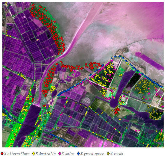
Figure 2.
The location map of samples for classification training and validation in Linhong Estuary.
2.3.2. Vegetation Types and the Image Characteristics
After image feature analysis and field surveying, the vegetation types were classified into five, including Spartina alterniflora (S. alterniflora), Phragmites australis (P. australis), Suaeda salsa (S. salsa), Road green space (R. green space), and Mixed weeds (M. weeds), as shown in Table 2.
Table 2.
Characteristics of each vegetation type on image of 24 June 2022 by 432 bands combination and their photos.
2.3.3. Vegetation Phenology Metric Construction
(1) Phenology time series construction.
NDVI was chosen to construct phenology metrics and then used as coastal wetland vegetation type classification features, because, among many image spectral characteristics, NDVI was the most widely adopted to draw phenology time series curves [12,30,50]. The NDVI values of all the samples collected at both Linhong Estuary and Liezi Estuary were calculated based on data in Table 1 and used for samples-based time series construction.
For five vegetation types, although there are differences in some of the phenology characteristics, for example, green-up ratio during spring season, NDVI maximum value during summer season, and senescence ratio during autumn season, the phenology cycles are identical and uniform with the four seasons. Therefore, we selected a two-term function to fit time series curves of the five vegetation types, and the formula is shown in Table 3.
Table 3.
The fitting curves of five vegetation types.
Table 3.
The fitting curves of five vegetation types.
| Vegetation Type | The Formula of Fitting Curves | R2 | RMSE |
|---|---|---|---|
| S. alterniflora | 0.9098 | 0.0716 | |
| P. australis | 0.827 | 0.0818 | |
| S. salsa | 0.9523 | 0.0186 | |
| R. green space | 0.934 | 0.0287 | |
| M. weeds | 0.8609 | 0.0967 |
In the formula, the x-coordinate indicates day of year (DOY) and the y-coordinate indicates the value of NDVI. w is the coefficient indicating the vegetation phenology cycle and is uniformly set to 0.017 (2π/365). The result is shown in Figure 3, and formulas of five vegetation fitting curves are shown in Table 3.

Figure 3.
The NDVI time series fitting curves of five vegetation types: the symbols of asterisks, dots, circles, squares and triangles indicate the mean NDVI values of S. alterniflora, P. australis, S. salsa, R. green space and M. weeds samples on corresponding images.
Figure 3.
The NDVI time series fitting curves of five vegetation types: the symbols of asterisks, dots, circles, squares and triangles indicate the mean NDVI values of S. alterniflora, P. australis, S. salsa, R. green space and M. weeds samples on corresponding images.

(2) Optimum windows for phenology metrics construction.
The fitting curves suggested that there are some keys of phenology timing at which different vegetation type NDVI values show a distinguished difference. However, it is difficult to acquire image data that was taken at the appropriate timing and to provide the largest separability for vegetation classification, as with the study of Sun [30] and Zhang [23] who used critical phenology timing images to discriminate plant species salt marshes. To adapt to the accessibility of HSR images, we constructed phenology metrics by images taken during optimum windows corresponding to different phenology phases instead of key timing points. According to the time series fitting curves, the optimum window was obtained as:
(1) Base value time window (Base value W)—the minimum NDVI value region of the fitting curves, which corresponds to winter season (late November to early April).
(2) Green-up time window (Green-up W)—the green-up period when P. australis starts to grow rapidly, while S. alterniflora is the stage of the base value or just starts to green up, corresponding to spring season (early April to late June).
(3) Maximum value time window (Maximum value W)—the maximum value of the fitting curve, which often occurs between late summer and early autumn (late June to early September).
(4) Senescence time window (Senescence W)—the senescence period when S. alterniflora is vigorous, while other vegetation types, especially P. australis, are in the process of or are into full senescence, corresponding to the autumn season (early September to late November).
(3) The construction of phenology metrics.
(1) Difference of NDVI (DON):
This metric is first constructed to enhance S. alterniflora and P. australis spectral differences. Of the metric variables, NDVIsenescence is calculated by images acquired during Senescence W and NDVIgreenup is calculated by images acquired during Green-up W.
(2) Ratio of green-up NDVI (ROGN):
This metric is primarily constructed to enhance P. australis spectral information using the green-up time window. Of the metric variables, NDVIgreenup is calculated by images acquired at Green-up W; NDVIbasevalue is calculated by images acquired at later Base value W.
(3) Ratio of senescence NDVI (ROSN):
This metric is constructed to further enhance S. alterniflora spectral information. Of the metric variables, NDVIsenescence is calculated by images acquired at Senescence W, and NDVIbasevalue is calculated by images acquired at early Base value W.
(4) Maximum of NDVI (MON)
This metric is calculated by images acquired in Maximum value W and it presents the maximum NDVI value of one kind of vegetation in four seasons.
(5) Sum of green-up and senescence NDVI (SON)
This metric is constructed to surrogate MON to further enhance S. alterniflora and P. australis spectral information, because it is difficult to take images at Maximum value W for cloudy weather. NDVIgreenup and NDVIsenescence are calculated by images acquired with the above-described methods.
2.3.4. Image Segment for Classification
According to the characteristic of HSR images, in this study, all the classifications were carried out based on object-oriented techniques [51]. Objects were obtained using multiple-scale segmentation by which continuous pixels grow up from bottom pixels to objects whose size and shape are determined by three parameters, including scale, shape, and compactness [52]. All the processes, including segmentation and classification, were performed by software Ecognition9.2.
2.3.5. Classification Algorithm
Two steps were employed to perform vegetation type classification: (1) At first, the threshold value method (Vegetation = NDVI ≥ 0.10) was carried out to discriminate vegetation with no vegetation based on object segmentation of 8 May 2022 using a scale of 100. (2) Then, vegetation areas were further classified by the Random Forest (RF) algorithm at the smaller segmentation scale of 60. The RF algorithm is an ensemble learning technique by which a classifier consisting of a collection of tree-structured classifiers and each tree casts a unit vote for the most popular class [53]. The RF algorithm is based upon the basic premise that a set of classifiers do perform better classifications than an individual classifier does. A tree of a RF grows from different training data subsets created through bagging or bootstrap aggregating [54].
2.3.6. Images Used for Phenology Metrics Calculation and Vegetation Type Classification
With the vegetation area segmentation result by the scale of 60, the RF algorithm was carried out to perform all classifying processes for its ensemble learning ability. Four images, corresponding to different optimized windows of one year, were used to construct phenology metrics to improve classification accuracy. The images, image features, and phenology metrics used for vegetation types classification are shown in Table 4. Compared with the single image of Green-up W or Senescence W, their combination can provide more features corresponding to certain vegetation types brought by different phenology phases. For the addition of four phenology metrics, DON was used to enlarge the difference between S. alterniflora or P. australis with other vegetation types. ROGN and ROSN were calculated to indicate the ratio of green-up in spring and the ratio of senescence in autumn. These metrics should be especially efficient for R. green space, which has a higher NDVI value than other vegetation types in winter. SON was used to identify the phenology characteristics of S. salsa for its lower NDVI value than any other vegetation types in the vigorous phase.
Table 4.
The images and their features used in vegetation type classification.
3. Results
3.1. Phenology Characteristics of Different Vegetation Types
As shown in Figure 3, the fitting curves of the NDVI time series reveal the tendency of changes in phenology for each vegetation type. The predominant characteristics include: (1) In Green-up W, P. australis starts to green-up rapidly and its NDVI value is higher than those of any other vegetation types. (2) In Senescence W, S. alterniflora is in the vigorous phenology phase and displays the highest NDVI value among all vegetation types. (3) M. weeds demonstrates a similar phenological cycle but lower NDVI value to that of P. australis. (4) In each phenological phase, S. salsa returns a lower NDVI value than the other vegetation types. (5) In winter, R. green space shows a higher NDVI value than other vegetation types.
Phenology metrics are constructed to identify the above characteristics. Illustrated as Figure 4, these metrics values of five vegetation types fluctuate in a certain range when the images used to calculate metrics are located in different positions of the optimized window. However, some common traits in favor of improving the classification result are obvious, including: (1) The DON value of S. alterniflora is higher than those of other vegetation types. (2) Both ROGN and ROSN values of R. green space tend to be lower than those of other vegetation types. (3) For five vegetation types, the values of MON and SON have similar comparison characteristics, which means SON can be used to surrogate MON, and the S. salsa value of both MON and SON is lowest among the five vegetation types.
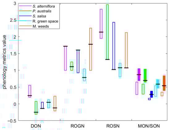
Figure 4.
The data range of phenology metrics. The wireframe filled with color indicates the value of MON, which is surrogated by SON and not used in this study. The black transverse lines on the wireframe indicate the phenology metrics value calculated by the four images in this study.
In this study, phenology metrics were calculated by four images, as shown as Table 4, and the phenology metrics mean value of samples is shown in Figure 4. Obviously, for these phenology metrics in this study, apart from the above common useful traits, some other helpful features could be obtained for improving the classification result, including the DON and ROGN value of P. australis, ROSN value of S. alterniflora, and SON value of P. australis and S. alterniflora.
3.2. Vegetation Type Classification and Accuracy Evaluation
If only by a single image, the confusion phenomena of the classification result are relatively serious. For example, in region (A) in Figure 5 of the classification result by the image taken in Green-up W, lots of pixels of S. alterniflora were classified as S. salsa, while in Figure 6 of the classification result by the image taken in Senescence W, they were classified as P. australis; for region (B), both in Figure 5 and Figure 6, many pixels of the S. salsa were classified as R. green space mistakenly. Among all vegetation types, R. green space was most frequently classified mistakenly; for example, in regions (C), (D), and (E), all pixels classified as R. green space were not identified correctly.
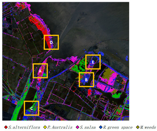
Figure 5.
Vegetation classification result by single image of 21 October 2020: (A) S. alterniflora classified as S. salsa mistakenly; (B) S. salsa classified as R. green space mistakenly; (C) P. australis classified as R. green space mistakenly; (D) S. alterniflora classified as R. green space mistakenly; (E) P. australis classified as R. green space mistakenly.
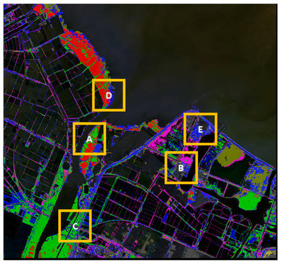
Figure 6.
Vegetation classification result by single image of 8 May 2021: (A) S. alterniflora classified as P. australis mistakenly; (B) S. salsa classified as R. green space mistakenly; (C) P. australis classified as R. green space mistakenly; (D) S. alterniflora classified as R. green space mistakenly; (E) P. australis classified as R. green space mistakenly.
The fitting curves of the NDVI time series revealed the tendency of changes in phenology for each vegetation type. From the curves’ changing tendency, the differing phenology characteristics of five vegetation types made it possible to extract the phenology metrics that were used to improve the vegetation type classification.
From Table 5, it can be shown that, if only by single image, because of the confusion phenomena, the classification accuracy was not high and the overall accuracy was 48% and 47%, respectively, and kappa was 34% and 33%, respectively. Among 5 vegetation types, S. alterniflora and P. australis were classified by higher accuracy than other vegetation types. By images of Green-up W, the classification accuracy of P. australis was highest, while by images of Senescence W, S. alterniflora acquired the highest classification accuracy. S. salsa and M. weeds were frequently confused with any other vegetation type, while every other vegetation was often classified as R. green space mistakenly.
Table 5.
Classification accuracy by single image.
When classification was carried out based on the combination of images taken in Green-up W and Senescence W, the classification accuracy was improved obviously, and the overall accuracy and kappa were improved to 67% and 58%, respectively (Table 5).
As shown in Figure 7, when combining two images, the improvement was mainly produced on regions where the vegetation presented an obvious domain pattern. For example, regions of (A), (C), and (F) belonged to the domain pattern of S. alterniflora, P. australis, and S. salsa, respectively; the omission error was decreased; then, their produce accuracy improved to 66%, 71%, and 61%. However, in some areas with complex vegetation growth conditions or structures, the confusion was also evident. For example, in region of (D), lots of pixels of P. australis were classified as M. weeds mistakenly, while in the entire study area, many pixels of various other vegetation types were mistakenly classified as R. green space.
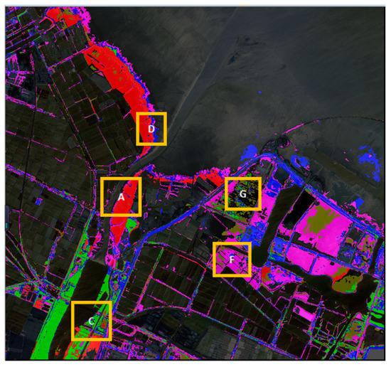
Figure 7.
Vegetation classification result with combination of two images: (A) S. alterniflora omission error decreased; (C) P. australis omission error decreased; (F) S. salsa omission error decreased; (D) S. alterniflora classified as R. green space mistakenly; (G) P. australis classified as M. weeds mistakenly.
When phenology metrics were added to the classification process, the most distinguished changes of the classification result was the improvement of R. green space’s discrimination, as its commission error was obviously decreased in the entire study area (Figure 8). Another evident improvement is shown as region (G), when only by the combination of two images taken on 8 May 2021 and 21 October 2020, the areas of P. australis and S. salsa were mistakenly classified as M. weeds as they were in the original development phase and presented low vegetation cover. When phenology metrics were combined with spectral information, M. weeds was efficiently discriminated from P. australis and S. salsa. In addition, in other areas, the classification result was also improved; for example, in region (F) on Figure 8, the confusion of S. salsa with M. weeds was decreased. However, in some areas, for example, region (H), the confusion between P. australis and R. green space was increased where P. australis grew around puddles and presented lower NDVI data with characteristics similar to R. green space’s. Finally, by evaluation, the overall accuracy and kappa were improved to 75% and 69%, respectively.
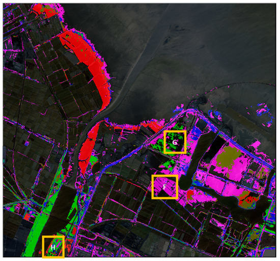
Figure 8.
Vegetation classification result by further addition of phenology metrics: (F) S. salsa classified correctly; (G) P. australis and S. salsa classified correctly; (H) P. australis classified as R. green space mistakenly.
4. Discussion
4.1. The Reasons Leading to Classification Error among Vegetation Types
Among the five vegetation types of interest in the study area, S. alterniflora, P. australis, and S. salsa were the three dominant species. The appearance of these species differed in various characteristics; therefore, combining their differing characteristics with their phenology differences in Green-up W or Senescence W might suggest that these species would be highly separable and should be discriminated clearly. However, as shown by the above classification results, if only by using a single image of Green-up W or Senescence W, the overall accuracy was 48% and 47%, respectively. The overall classification accuracy was obviously improved to 67% by combining images of the two optimization windows for areas, where vegetation was flourishing and displayed an obvious dominance pattern. In other areas, the confusion phenomena of the classification result were also obvious, for example, the user accuracy of R. green space was only 31%.
From our analysis of the classification error in combining the land-use characteristics in the study area, we arrived at two explanations for the observed decrease in classification accuracy.
(1) Strong and continuing disturbance of human activities. Such disturbances caused complex vegetation composition, such as the fragmented patches composed of P. australis with S. salsa and M. weeds (Figure 9a), the expansion of different M. weeds (Figure 9b), or the emergence of different vegetation succession phases (Figure 9c). It is worth mentioning among all the causes of disturbance is the emergence of R. green space (Figure 9e,f), featuring a complex composition and displaying similar spectral characteristics to those of S. alterniflora in senescence W, yet resembling P. australis in Green-up W.
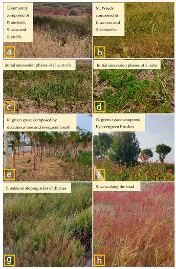
Figure 9.
The on-site situations leading to classification error among vegetation types: in photo (a), S. viridis is the abbreviation of Setaria viridis (Linn.) Beauv.; in photo (b), E. annuus and S. cannabinais are the abbreviations of Erigeron annuus (Linn.) Pers. and Sesbania cannabina (Retz.) Poir., respectively.
(2) Vegetation spectral instability induced by different microclimate conditions. For example, S. salsa, during the growth process, changed in stem color and form according to the environment (such as unused salt ponds, the sloping sides of ditches, or along the road near fishponds), producing differences even in the same phenology timing (Figure 9g,h).
4.2. Efficiency of Phenology Metrics for above Disadvantages for Vegetation Type Classification
Adding four phenology metrics to the classification process directly improved the vegetation classification results in comparison to the classification results acquired by the direct combination of images of 8 May 2021 and 21 October 2020.
The most significant improvement acquired was to discriminate R. green space. From Figure 8, the phenomenon of its misclassification in a large area shown in Figure 7 decreased; as shown in Table 5, the user accuracy improved from 31% to 52%. The second prominent improvement was about the M. weeds misclassification with P. australis or S. salsa, as shown in Figure 8. In addition, there were also some improvements for other situation, for example, between the S. alterniflora and M. weeds. With these improvements, most of the produce and user accuracy were increased at different levels, and the overall accuracy and kappa reached to 75% and 69% from 67% and 58%, when phenology metrics were added to the combination of images of Green-up W and Senescence W. These improvements displayed the efficiency of phenology metrics for dealing with the above disadvantages for vegetation classification.
However, in some areas, such as region (H), the confusion between P. australis and R. green space was increased, where P. australis grew around puddles and yielded lower NDVI data values that showed characteristics similar to R. green space.
4.3. Significance of This Study for Estuarine Wetlands Vegetation Type Classification
Although HSR satellite images are advanced data for estuarine wetlands vegetation type classification, because of its multi-spectral information and fine spatial detail, their temporal resolution is not high enough to satisfy the need of phenology time series fitting when used for vegetation type classification. This study was constructed to deal with this conflict, with the advent of China GF series satellites. With these high spatial images, although we cannot acquire high-temporal-resolution satellite images, it is practical to obtain a certain number of images taken in spring, autumn, and winter within one year, and these times are located in three optimized windows that could be used to calculate phenology metrics constructed in this study.
In this study, we acquired four scene images taken in Base value W, Green-up W, and Senescence W, respectively, to calculate phenology metrics to improve the vegetation type classification result. The study results demonstrate that these metrics could obviously increase the estuarine wetland vegetation type classification accuracy; therefore, this research provides efficient approaches for combing spectral information with phenology features to obtain satisfying estuarine vegetation type classification results for ecological system management and protection.
Though the advantages of combining phenology metrics with spectral features is evident, some limitations were also obvious. In the future, with the progress of remote sensing technology, the accessibility of high-spatial-resolution images would be increased, and these questions will be further studied by exploring the selection of images taken in more appropriate times, determining more precisely optimized windows, and developing more reasonable phenology metrics.
5. Conclusions
In this study, four phenology metrics were constructed according to phenology time series fitting curves using samples selected from two areas, the Linhong Estuary Wetland and Liezi Estuary Wetland, based on images taken during a five-year period (2018–2022). After evaluating and analyzing the classification results, we drew the following conclusions:
(1) Differences in vegetation phenology characteristics provided a feasible approach for phenology metrics construction. In this study, five vegetation types had obvious phenology timing that produced four optimized windows, as follows: Base value W, Maximum value W, Green-up W, and Senescence W. During each optimized window, the characteristics of the five vegetation types corresponded to different phenology features, which allowed the construction of various phenology metrics for discriminating between vegetation types, including Difference of NDVI (DON), Ratio of green-up NDVI (ROGN), Ratio of senescence NDVI (ROSN), and Sum of green-up and senescence NDVI (SON).
(2) The phenology metrics had an evident positive effect on the vegetation type classification results. Compared to classification using only a single image taken in Green-up W or Senescence W, adding the metrics to the classification procedure obviously improved the accuracy of the classification of the vegetation types. Combining the images provided better vegetation classification accuracy than any single image. This improvement mainly occurred in regions where each vegetation type was obviously dominant and in a flourish growth state. Adding phenology metrics to the classification process could overcome some confusing phenomena caused by changing growth conditions to some extent, especially in the case of R. green space, and further improved the classification accuracy.
(3) This study’s results offer some benefits for the classification of coastal wetland vegetation using GF series satellite imagery. However, limitations are also evident, and many problems require further study. Recommended studies include the accumulation of additional images and samples that precisely describe the vegetation phenology timing, as well as images taken at more appropriate times to carry out classification tasks. Additional investigation is also needed to develop more reasonable phenology metrics and more advanced classification methods to achieve higher classification accuracy.
Author Contributions
Conceptualization, Z.H. and Y.Z.; methodology, Y.G. (Yu Gao); software, Q.S.; validation, Z.W., D.C. and Y.G. (Yajun Gao); formal analysis, D.C. and S.W.; investigation, Y.G. (Yu Gao); resources, S.W.; data curation, Y.G. (Yu Gao); writing—original draft preparation, Y.G. (Yu Gao); writing—review and editing, Z.H. and Y.Z.; visualization, Z.W.; supervision, Z.H.; project administration, Z.H.; funding acquisition, Z.H. All authors have read and agreed to the published version of the manuscript.
Funding
China GF series satellites data are highly appreciated. This research was funded by the Key Laboratory of Coastal Salt Marsh Ecology and Resources, Ministry of Natural Resources (KLCSMERMNR2021102), the National Natural Science Foundation of China (NSFC Nos. 52074133; 31270745), A Project Funded by the Priority Academic Program Development of Jiangsu Higher Education Institutions (PAPD) of Jiangsu Normal University; the Key subject of “Surveying and Mapping Science and Technology” of Jiangsu Ocean University (KSJOU), Postgraduate Research & Practice Innovation Program of Jiangsu Normal University (2021XKT0085).
Institutional Review Board Statement
Not applicable.
Informed Consent Statement
Not applicable.
Data Availability Statement
All China GF series satellites data are available at http://www.sasclouds.com/chinese/normal/ (accessed on 26 April 2022).
Acknowledgments
China GF series satellites data are highly appreciated.
Conflicts of Interest
The authors declare no conflict of interest.
References
- Kimball, J. Vegetation Phenology. In Encyclopedia of Remote Sensing; Njoku, E.G., Ed.; Springer New York: New York, NY, USA, 2014; pp. 886–890. [Google Scholar]
- Katharine, W.; Jennifer, P.; Paul, S. Remote sensing of spring phenology in northeastern forests: A comparison of methods, field metrics and sources of uncertainty. Remote Sens. Environ. 2014, 148, 97–107. [Google Scholar]
- Berra, E.F.; Gaulton, R. Remote sensing of temperate and boreal forest phenology: A review of progress, challenges and op-portunities in the intercomparison of in-situ and satellite phenological metrics. For. Ecol. Manag. 2021, 480, 118663. [Google Scholar] [CrossRef]
- Zhang, X.; Friedl, M.A.; Schaaf, C.B.; Strahler, A.H.; Hodges, J.C.; Gao, F.; Reed, B.C.; Huete, A. Monitoring vegetation phenology using MODIS. Remote Sens. Environ. Interdiscip. J. 2003, 84, 471–475. [Google Scholar] [CrossRef]
- Zhang, X. Reconstruction of a complete global time series of daily vegetation index trajectory from long-term AVHRR data. Remote. Sens. Environ. 2015, 156, 457–472. [Google Scholar] [CrossRef]
- Atkinson, P.M.; Jeganathan, C.; Dash, J.; Atzberger, C. Inter-comparison of four models for smoothing satellite sensor time-series data to estimate vegetation phenology. Remote Sens. Environ. 2012, 123, 400–417. [Google Scholar] [CrossRef]
- Vrieling, A.; Skidmore, A.K.; Wang, T.; Meroni, M.; Ens, B.J.; Oosterbeek, K.; O’Connor, B.; Darvishzadeh, R.; Heurich, M.; Shepherd, A.; et al. Spatially detailed retrievals of spring phenology from single-season high-resolution image time series. Int. J. Appl. Earth Obs. Geoinf. 2017, 59, 19–30. [Google Scholar] [CrossRef]
- Vrieling, A.; Meroni, M.; Darvishzadeh, R.; Skidmore, A.K.; Wang, T.; Zurita-Milla, R.; Oosterbeek, K.; O’Connor, B.; Paganini, M. Vegetation phenology from Sentinel-2 and field cameras for a Dutch barrier island. Remote Sens. Environ. 2018, 215, 517–529. [Google Scholar] [CrossRef]
- Zeng, L.; Wardlow, B.D.; Xiang, D.; Hu, S.; Li, D. A review of vegetation phenological metrics extraction using time-series, multispectral satellite data. Remote Sens. Environ. 2020, 237, 111511. [Google Scholar] [CrossRef]
- Son, N.-T.; Chen, C.-F.; Chen, C.-R.; Duc, H.-N.; Chang, L.-Y. A Phenology-Based Classification of Time-Series MODIS Data for Rice Crop Monitoring in Mekong Delta, Vietnam. Remote Sens. 2013, 6, 135–156. [Google Scholar] [CrossRef]
- David, H.; Itamar, L.; Naama, T.; Yagil, O. A Phenology-Based Method for Monitoring Woody and Herbaceous Vegetation in Mediterranean Forests from NDVI Time Series. Remote Sens. 2015, 7, 12314–12335. [Google Scholar]
- Eli, K.M.; Damien, S.; Josh, M.G.; Black, T.A.; Timothy, H.M.; Andrew, D.R.; Mark, A.F. Multisite analysis of land surface phenology in North American temperate and boreal deciduous forests from Landsat. Remote Sens. Environ. 2016, 186, 452–464. [Google Scholar]
- Feng, G.; Martha, C.A.; Xiaoyang, Z.; Zhengwei, Y.; Joseph, G.A.; William, P.K.; Rick, M.; David, M.J.; John, H.P. Toward mapping crop progress at field scales through fusion of Landsat and MODIS imagery. Remote Sens. Environ. 2017, 188, 9–25. [Google Scholar]
- Nijland, W.; Bolton, D.; Coops, N.; Stenhouse, G. Imaging phenology; scaling from camera plots to landscapes. Remote Sens. Environ. 2016, 177, 13–20. [Google Scholar] [CrossRef]
- Fisher, J.I.; Mustard, J.F.; Vadeboncoeur, M.A. Green leaf phenology at Landsat resolution: Scaling from the field to the satellite. Remote Sens. Environ. 2006, 100, 265–279. [Google Scholar] [CrossRef]
- Walker, J.J.; de Beurs, K.M.; Wynne, R.H. Dryland vegetation phenology across an elevation gradient in Arizona, USA, investigated with fused MODIS and Landsat data. Remote Sens. Environ. 2014, 144, 85–97. [Google Scholar] [CrossRef]
- Frantz, D.; Stellmes, M.; Röder, A.; Udelhoven, T.; Mader, S.; Hill, J. Improving the Spatial Resolution of Land Surface Phenology by Fusing Medium- and Coarse-Resolution Inputs. IEEE T Geosc. Remote 2016, 54, 4153–4164. [Google Scholar] [CrossRef]
- Patrick, G.; Claas, N.; Patrick, H. Intra-annual reflectance composites from Sentinel-2 and Landsat for national-scale crop and land cover mapping. Remote Sens. Environ. 2019, 220, 135–151. [Google Scholar]
- Zhang, X.; Xiao, X.; Wang, X.; Xu, X.; Chen, B.; Wang, J.; Ma, J.; Zhao, B.; Li, B. Quantifying expansion and removal of Spartina alterniflora on Chongming island, China, using time series Landsat images during 1995–2018. Remote Sens. Environ. 2020, 247, 111916. [Google Scholar] [CrossRef]
- Xu, R.; Zhao, S.; Ke, Y. A Simple Phenology-Based Vegetation Index for Mapping Invasive Spartina Alterniflora Using Google Earth Engine. IEEE J. Sel. Top. Appl. Earth Obs. Remote Sens. 2020, 14, 190–201. [Google Scholar] [CrossRef]
- Rufin, P.; Frantz, D.; Ernst, S.; Rabe, A.; Griffiths, P.; Özdoğan, M.; Hostert, P. Mapping Cropping Practices on a National Scale Using Intra-Annual Landsat Time Series Binning. Remote Sens. 2019, 11, 232. [Google Scholar] [CrossRef]
- Grabska, E.; Frantz, D.; Ostapowicz, K. Evaluation of machine learning algorithms for forest stand species mapping using Sentinel-2 imagery and environmental data in the Polish Carpathians. Remote Sens. Environ. 2020, 251, 112103. [Google Scholar] [CrossRef]
- Bendini, H.D.N.; Fonseca, L.M.G.; Schwieder, M.; Körting, T.S.; Rufin, P.; Sanches, I.D.A.; Leitão, P.J.; Hostert, P. Detailed agricultural land classification in the Brazilian cerrado based on phenological information from dense satellite image time series. Int. J. Appl. Earth Obs. Geoinf. 2019, 82, 101872. [Google Scholar] [CrossRef]
- Hemmerling, J.; Pflugmacher, D.; Hostert, P. Mapping temperate forest tree species using dense Sentinel-2 time series. Remote Sens. Environ. 2021, 267, 112743. [Google Scholar] [CrossRef]
- Ai, J.; Gao, W.; Gao, Z.; Shi, R.; Zhang, C. Phenology-based Spartina alterniflora mapping in coastal wetland of the Yangtze Estuary using time series of GaoFen satellite no. 1 wide field of view imagery. J. Appl. Remote Sens. 2017, 11, 026020. [Google Scholar] [CrossRef]
- Sun, C.; Li, J.; Liu, Y.; Liu, Y.; Liu, R. Plant species classification in salt marshes using phenological parameters derived from Sentinel-2 pixel-differential time-series. Remote Sens. Environ. 2021, 256, 112320. [Google Scholar] [CrossRef]
- Wang, M.; Fei, X.; Zhang, Y.; Chen, Z.; Wang, X.; Tsou, J.Y.; Liu, D.; Lu, X. Assessing Texture Features to Classify Coastal Wetland Vegetation from High Spatial Resolution Imagery Using Completed Local Binary Patterns (CLBP). Remote Sens. 2018, 10, 778. [Google Scholar] [CrossRef]
- Yokoya, N.; Grohnfeldt, C.; Chanussot, J. Hyperspectral and Multispectral Data Fusion: A comparative review of the recent literature. IEEE Geosci. Remote Sens. 2017, 5, 29–56. [Google Scholar] [CrossRef]
- Li, Q.; Wong, F.K.K.; Fung, T. Mapping multi-layered mangroves from multispectral, hyperspectral, and LiDAR data. Remote Sens. Environ. 2021, 258, 112403. [Google Scholar] [CrossRef]
- Takeshi, S.; Junichi, I.; Keiko, I.; Yukihiro, M.; Katsunori, K. Object-based classification of land cover and tree species by integrating airborne LiDAR and high spatial resolution imagery data. Landsc. Ecol. Eng. 2012, 8, 157–171. [Google Scholar]
- Hill, R.A.; Wilson, A.K.M.; Hinsley, G.S.A. Mapping tree species in temperate deciduous woodland using time series multispectral data. Appl. Veg. Sci. 2010, 13, 86–99. [Google Scholar] [CrossRef]
- Tigges, J.; Lakes, T.; Hostert, P. Urban vegetation classification: Benefits of multitemporal RapidEye satellite data. Remote Sens. Environ. 2013, 136, 66–75. [Google Scholar] [CrossRef]
- Li, D.; Ke, Y.; Gong, H.; Li, X. Object-Based Urban Tree Species Classification Using Bi-Temporal WorldView-2 and WorldView-3 Images. Remote Sens. 2015, 7, 16917–16937. [Google Scholar] [CrossRef]
- Yan, J.; Zhou, W.; Han, L.; Qian, Y. Mapping vegetation functional types in urban areas with WorldView-2 imagery: Integrating object-based classification with phenology. Urban Urban Gree 2018, 31, 230–240. [Google Scholar] [CrossRef]
- Li, Z.; Zhang, Q.Y.; Qiu, X.C.; Peng, D.L. Temporal stage and method selection of tree species classification based on GF-2 remote sensing image. Chin. J. Appl. Ecol. 2019, 30, 4059–4070. [Google Scholar]
- Wang, E.L.; Li, C.J.; Zhou, J.P.; Peng, D.L.; Hu, H.T.; Dong, X. Classification of Beijing Afforestation Species Based on Multi-temporal Images. J. Beijing Univ. Technol. 2017, 43, 710–718. [Google Scholar]
- Gedan, K.B.; Kirwan, M.L.; Wolanski, E.; Barbier, E.B.; Silliman, B. The present and future role of coastal wetland vegetation in protecting shorelines: Answering recent challenges to the paradigm. Clim. Chang. 2010, 106, 7–29. [Google Scholar] [CrossRef]
- Shuai, Z.; Shuai, G.; Ning, L.; Zheng, W. Community structure and diversity of overwintering waterbirds in four estuarine wetlands of Lianyungang City. J. Ecol. Rural. Environ. 2020, 36, 560–566. [Google Scholar]
- Victor, K. Using Remote Sensing to Select and Monitor Wetland Restoration Sites: An Overview. J. Coast. Res. 2013, 29, 958–970. [Google Scholar]
- Gao, X.; Fei, X.; Soldiers, K. Object-oriented analysis of land use change and driving forces in lianyungang coastal zone. Mar. Sci. 2014, 38, 81–87. [Google Scholar]
- Fei, X.; He, X.; Xie, H.; Wang, H.; Chen, S.; Chen, T. Remote Sensing Classification of Linhong Estuary Wetlands Based on GF-1 Satellite Image. J. Jiangsu Ocean Univ. Nat. Sci. Ed. 2021, 30, 50–57. [Google Scholar]
- Bai, Z. GF-1 Satellite—The First Satellite of CHEOS. Aerosp. China 2013, 14, 11–16. [Google Scholar]
- Huang, W.; Sun, S.; Jiang, H.; Gao, C.; Zong, X. GF-2 Satellite 1m/4m Camera Design and In-Orbit Commissioning. Electron. J. Engl. 2018, 27, 1316–1321. [Google Scholar] [CrossRef]
- Ren, K.; Sun, W.; Meng, X.; Yang, G.; Du, Q. Fusing China GF-5 Hyperspectral Data with GF-1, GF-2 and Sentinel-2A Multi-spectral Data: Which Methods Should Be Used? Remote Sens. 2020, 12, 882. [Google Scholar] [CrossRef]
- Li, Y.; Yang, Y.; Zhu, X. A preliminary study on the functional zoning of lianyungang coastal zone. Coast. Eng. 2001, 4, 43–50. [Google Scholar]
- Xu, X.; Liu, Y.; Ran, S. Analysis on Change Trend of Evaporation in Lianyungang City. Adm. Huaihe River 2008, 9, 6–7. [Google Scholar]
- Li, H.; Li, C.; Shen, Y.; Li, H.; Li, F.; Jiang, J. Study on the Ecological Distribution Characteristics and Growth Competitiveness of Suaeda salsa in Beach Salt Land. Jiangsu Agric. Sci. 2009, 2, 296–298. [Google Scholar]
- You, C.; Mo, X.; Zhang, S.; Zheng, Y.; Liu, F. Ecological stoichiometric characteristics of different plant communities at the mouth of the Meihe River in Duliu, Tianjin. Chin. J. Appl. Environ. Biol. 2019, 25, 617–625. [Google Scholar]
- Chen, D.; Fei, X.; Wang, Z.; Gao, Y.; Shen, X.; Han, T.; Zhang, Y. Classifying Vegetation Types in Mountainous Areas with Fused High Spatial Resolution Images: The Case of Huaguo Mountain, Jiangsu, China. Sustainability 2022, 14, 13390. [Google Scholar] [CrossRef]
- Yan, J.; Guo, J. Extraction and Analysis of Natural Vegetation Cover and Soil Moisture Using Landsat TM Data in the Arid Oasis of Xinjiang, China. J. Indian Soc. Remote Sens. 2019, 47, 213–221. [Google Scholar] [CrossRef]
- Blaschke, T.; Burnett, C.; Pekkarinen, A. Image Segmentation Methods for Object-based Analysis and Classification; Springer: Dordrecht, The Netherlands, 2004; pp. 211–236. [Google Scholar]
- Chen, Z.; Fei, X.; Gao, X.; Wang, X.; Zhao, H.; Wong, K.; Tsou, J.; Zhang, Y. The Influence of CLBP Window Size on Urban Vegetation Type Classification Using High Spatial Resolution Satellite Images. Remote Sens. 2020, 12, 3393. [Google Scholar] [CrossRef]
- Breiman, L. Random Forests. Mach Learn. 2001, 45, 5–32. [Google Scholar] [CrossRef]
- Wang, X.; Gao, X.; Zhang, Y.; Fei, X.; Chen, Z.; Wang, J.; Zhang, Y.; Lu, X.; Zhao, H. Land-Cover Classification of Coastal Wetlands Using the RF Algorithm for Worldview-2 and Landsat 8 Images. Remote Sens. 2019, 11, 1927. [Google Scholar] [CrossRef]


Disclaimer/Publisher’s Note: The statements, opinions and data contained in all publications are solely those of the individual author(s) and contributor(s) and not of MDPI and/or the editor(s). MDPI and/or the editor(s) disclaim responsibility for any injury to people or property resulting from any ideas, methods, instructions or products referred to in the content. |
© 2023 by the authors. Licensee MDPI, Basel, Switzerland. This article is an open access article distributed under the terms and conditions of the Creative Commons Attribution (CC BY) license (https://creativecommons.org/licenses/by/4.0/).