Examining the Factors Influencing Agricultural Surface Source Pollution in the Yangtze River Economic Zone from the Perspectives of Government, Enterprise, and Agriculture

Abstract

In this study, for the period between 2006 and 2021, we used the spatial Durbin model and dynamic Generalized Method of Moments to analyze the spatial and temporal characteristics and contributory factors of agricultural surface source pollution in 11 provinces and cities within China’s Yangtze River Economic Belt from the perspectives of governments, enterprises, and farmers. In addition, we also investigated the threshold characteristics of the distortion of the factor market for agricultural surface source pollution under different levels of environmental regulation. Our results revealed a positive spatial correlation between agricultural surface pollution in the Yangtze River Economic Belt which was significant at the 1% level. Furthermore, we established that government environmental regulation, input factor market distortion, and labor transfer have significant effects on agricultural surface pollution, among which factor market distortion has a significant spatial spillover effect in this economic zone, and environmental regulation has a significant single-threshold effect, with a threshold value of 0.1405. Based on these findings, we propose practical steps for the mitigation of agricultural surface pollution from the perspectives of governments, enterprises, and farmers which could be adopted to support countryside revitalization.

1. Introduction

As a major agricultural country, China has made significant progress in agricultural development in recent years. According to the Ministry of Agriculture and Rural Development, China’s total trade in agricultural products in 2006 amounted to $63.48 billion and has shown a rising trend in the past 16 years, reaching a figure of $334.32 billion in 2022 [1]. However, as the scale of China’s agricultural trade continues to expand, it is increasingly becoming a source of serious environmental problems, among which agricultural surface pollution has been identified as an important factor hindering the sustainable development of the country’s agricultural production. Moreover, these pollutants can also damage the soil structure, cause fires, and pollute the air environment which in turn have an impact on health. According to China’s seventh population census, 40% of all cancers occur in rural areas, where the resident population is only half that of towns and cities. At present, the relevant authorities and measures implemented to tackle agricultural surface pollution in China are characterized by decentralization, uncertainty, and delay [2]. Indeed, it is difficult to identify the main body responsible for the management of agricultural pollution and supervision of the process of governance, thereby resulting in insufficient participation by the main body and an unsatisfactory governance effect. Currently, the prevention and control of agricultural surface pollution in China is far from satisfactory. For a prolonged period of time, the Yangtze River Economic Zone—considered the most important agricultural production base in China—has been a region of rapid economic growth. However, the degree of agricultural surface pollution is concomitantly increasing, which is severely restricting the sustainable economic development and ecological protection of this economic zone. Accordingly, as a key area of concern for the green development of agriculture in this new environmentally aware era, in this study, we selected panel data for the Yangtze River Economic Belt for empirical analysis [3].

Given that the agricultural environment has the attributes of public goods, governments should in theory be the main governing bodies addressing the problem of agricultural surface pollution, and the environmental regulations these governments adopt largely influence whether the problem of agricultural surface pollution can be effectively solved [4]. As far as the market is concerned, failure of the input factor market exacerbates the use of inferior products by farmers to a certain extent, thereby contributing further to agricultural surface pollution. In the context of China’s large national population, the pressure of market demand for agricultural security, and small-scale agricultural operations, farmers comprise the largest number of agricultural producers with the largest total production and operation area and are consequently considered the major source of agricultural surface pollution [5].

Our group—in the book “Research on Lake Protection Strategies in Northern Jiangsu” [6]—selected farmers in Jinhu County, Huai’an City, Jiangsu Province, China as the survey object, resulting in 240 questionnaires being distributed, 238 recovered—excluding duplicates and incomplete invalid questionnaires—and 162 used as valid questionnaires; the questionnaire validity rate was 68%. The results of the questionnaire showed that 8% of the farmers chose to rely very much on fertilizers, 33% chose to rely generally on fertilizers, 24% chose to rely on fertilizers, 19% chose to rely slightly on fertilizers, and 16% chose not to rely on fertilizers during planting, which indicates that farmers in the region still rely on fertilizers to a high degree at this stage to obtain high output and high yields. According to the Ministry of Agriculture and Rural Affairs of the People’s Republic of China [7], chemical oxygen demand (COD), total nitrogen (TN), and total phosphorus (TP) have been identified as the main pollution load indicators of agricultural non-point source pollution. Existing literature [8,9] analyzed the main sources of agricultural non-point source pollution through clustering analysis and concluded that the main sources of agricultural non-point source pollutants TN and TP in China consist of livestock and poultry manure and farmland cultivation. Although the pollution situation varies from province to province, these two pollutants combined account for the majority of the pollution, exceeding 90%.

Researchers in both China and other countries have expended considerable effort in assessing the problem of agricultural surface pollution and the factors contributing to this pollution from several different perspectives. From a governmental perspective, studies have shown that an improvement in the intensity of government environmental management is conducive to an improvement in its efficacy [10]. Similar studies have also confirmed that the development of appropriate environmental regulations is an important strategy for curbing agricultural surface pollution [11,12,13]. For example, to effectively reduce the degree of agricultural surface pollution, governments can use agricultural insurance as an important policy tool to promote the green transformation of agricultural practices [14]. Environmental regulatory policies can also promote advances in agricultural production technology; for example, via the implementation of environmental regulatory policies that tax firms that pollute beyond prescribed limits. This approach accordingly aims to incentivize firms to adopt innovative technological approaches, thereby enhancing their environmental performance and competitiveness, and consequently reducing the degree of agricultural surface source pollution [15]. From a market perspective, the studies conducted to date have mainly focused on analyzing input factor markets. With progress in the development of agricultural technology, there has been an increase in the input of agricultural production factors within the market, which has brought about larger-scale agricultural production and exacerbated the problem of agricultural surface pollution [16]. Furthermore, from the perspectives of the chemical fertilizer market and agricultural labor force, several scholars have assessed the impact of fertilizer market distortion and reductions in the rural labor force on the application of chemical fertilizers by farmers, and, ultimately, the exacerbation of agricultural surface pollution [17,18,19].

Based on the foregoing considerations, in this study, where we focus on the Yangtze River Economic Belt, we developed an econometric model to examine the spatial and temporal characteristics and contributory factors of agricultural surface pollution from the multiple perspectives of government, market, and farmers. The main contributions and innovations of this study are as follows. Firstly, we focus on the Yangtze River Economic Belt in China, rather than on a specific province or city, and assess the current status of agricultural surface pollution in the region to provide policy recommendations for the realization of sustainable economic and ecological development. Secondly, we examine the impacts of environmental regulations, factor market distortion, and labor transfer on agricultural surface pollution from the perspectives of the government, market, and farmers, which provides new insights into this problem. Thirdly, to provide targeted suggestions for the promotion of pollution management and realization of rural revitalization, we employed spatial Durbin and threshold effect models to examine the spatial spillover effect of factor market distortion. This means that factor prices no longer truly reflect the effects of the scarcity of factor resources and the value of products on agricultural surface pollution and its threshold effect on this pollution under different intensities of environmental regulation. Fourthly, considering the time lag and negative externalities of environmental pollution, we evaluated the robustness of our analysis using a dynamic GMM method, which takes into account the effects of the lagged term, thereby correcting this error and enabling us to present more credible conclusions.

2. Materials and Methods

2.1. Research Methodology

2.1.1. Spatial Autocorrelation Model

Prior to performing spatial econometric regression, it was necessary to establish the spatial autocorrelation of agricultural surface pollution in the Yangtze River Economic Belt. In this regard, we used the global and local Moran indices to enable a more comprehensive characterization of the spatial distribution and aggregation of agricultural surface pollution in the Yangtze River Economic Zone as a whole and the different provinces and cities within this zone. Before calculating these Moran indices, it is initially essential to determine the spatial weight matrix, the main selection methods of which are based on collinearity and distance. Given that the provinces and cities in the Yangtze River Economic Belt analyzed in this study have common boundaries, we selected the 0–1 neighboring weight matrix W, the formula of which is expressed as follows:

Spatial weighting matrix:

$${\mathrm{W}}_{ij}=\left\{\begin{array}{c}1,\mathrm{regions}i\mathrm{and}j\mathrm{are}\mathrm{adjacent}\\ 0,\mathrm{regions}i\mathrm{and}j\mathrm{are}\mathrm{not}\mathrm{adjacent}\end{array}\right.$$

(1)

Global Moran I index:

$${\mathrm{M}\mathrm{o}\mathrm{r}\mathrm{a}\mathrm{n}}^{}\mathrm{I}=\frac{{\sum }_{i=1}^n\sum _{j=1}^n{W}_{ij}\left(x_i-\overline{x}\right)\left(x_j-\overline{x}\right)}{S^2{\sum }_{i=1}^n\sum _{j=1}^n{W}_{ij}}$$

(2)

Lisa index:

$$I_i=\frac{y_i-\overline{y}}{S^2}\sum _{j=1}^n{W}_{ij}\left(y_i-\overline{y}\right)$$

(3)

$$S^2=\frac{1}{n}\sum _{i=1}^n{\left(y_i-\overline{y}\right)}^2,\overline{y}=\frac{1}{n}\sum _{i=0}^n{y}_i,$$

(4)

where x_i and x_j are the observed sample values of provinces i and j, respectively; n is the number of provinces and cities; S² is the sample variance; and w_ij is the spatial weight matrix. When there is a neighboring boundary between city i and city j, w_ij is recorded as 1, whereas if there is no neighboring boundary, it is recorded as 0. The Moran I index takes a value between −1 and 1, with a larger absolute value being indicative of a stronger spatial correlation.

2.1.2. Spatial Durbin Model

To further examine the factors influencing agricultural surface pollution in the Yangtze River Economic Belt from the three perspectives of government, enterprise, and agriculture, based on reference to previous studies [20,21], we employed a spatial Durbin model (SDM) to analyze the influences of the explanatory variables on agricultural surface pollution, the expression of which is as follows:

$$\begin{array}{ll}Ln{P}_{it}={\beta }_0+& \rho W_{ij}Ln{P}_{it}+{\beta }_1{ER}_{it}+{\beta }_2{D}_{it}+{\beta }_3{LM}_{it}+{\beta }_4{Control}_{it}+{\delta }_1{W}_{ij}{ER}_{it}+{\delta }_2{W}_{ij}{D}_{it}+{\delta }_3{W}_{ij}{LM}_{it}\\ & +{\delta }_4{W}_{ij}{Control}_{it}+{\mu }_i+v_t+{\epsilon }_{it,}\end{array}$$

(5)

where the subscripts i and t denote province and year, respectively, P_it is the explanatory variable for agricultural surface pollution, E_Rit is environmental regulation, D_it represents fertilizer factor market distortion, LM_it is labor migration, Control_it is the control variable, and W_ij is the spatial weight matrix. β is the corresponding coefficient which represents the effect and degree of influence of each variable on the dependent variable, ρ is the spatial autocorrelation coefficient representing the extent to which data have a stronger correlation the closer the distance between geographic locations, u_i is the individual effect which used to capture differences between individuals that do not change over time, vi is the temporal effect which is used to solve with respect to omitted variables that do not change with individuals but change over time, and ε_it is the residual which refers to the difference between the actual observed value and the estimated value.

2.1.3. GMM Methods for Dynamic Systems

To avoid problems associated with endogeneity that may arise from the use of traditional static models, we introduced a term reflecting the lag in agricultural surface pollution as an explanatory variable based on Equation (8), and the dynamic systematic GMM method was used to perform a robustness test, which is given by the following formula:

$$Ln{P}_{it}=\alpha +{\beta }_{0}Ln{P}_{i,t-1}+{\beta }_1{ER}_{it}+{\beta }_2{D}_{it}+{\beta }_3{LM}_{it}+{\beta }_4{Control}_{it}+{\mu }_i+v_t+{\epsilon }_{it},$$

(6)

where P_{i, t−1} denotes the lag period for agricultural surface pollution. The remaining variables used in Equation (6) correspond to those used in Equation (5) and are not defined here [22].

2.1.4. Threshold Model

To further examine the non-linear impact of factor market distortion on agricultural surface pollution, we modified Hansen’s [23] threshold effect test to construct a threshold model with environmental regulation as the threshold variable using the following formula:

$$\begin{array}{ll}\mathrm{L}\mathrm{n}{\mathrm{P}}_{\mathrm{i}\mathrm{t}}={\beta }_0+& {\beta }_1{\mathrm{D}}_{\mathrm{i}\mathrm{t}}\times \mathrm{K}\left({\mathrm{E}\mathrm{R}}_{\mathrm{i}\mathrm{t}}\le {\tau }_1\right){+}^{\dots }{+\beta }_n{\mathrm{D}}_{\mathrm{i}\mathrm{t}}\times \mathrm{K}\left({\tau }_{n-1}<{\mathrm{E}\mathrm{R}}_{\mathrm{i}\mathrm{t}}\le {\tau }_n\right)+{\beta }_{n+1}{\mathrm{D}}_{\mathrm{i}\mathrm{t}}\times \mathrm{K}\left({\mathrm{E}\mathrm{R}}_{\mathrm{i}\mathrm{t}}>{\tau }_n\right)+{\beta }_c{\mathrm{C}\mathrm{o}\mathrm{n}\mathrm{t}\mathrm{r}\mathrm{o}\mathrm{l}}_{\mathrm{i}\mathrm{t}}\\ & +{\epsilon }_{it},\end{array}$$

(7)

where τ is the threshold to be estimated and K(…) is a schematic function. If the expression within the parentheses is true, it is assigned a value of 1; otherwise, it is designated as 0.

2.2. Variable Selection and Data Sources

Our analysis of the factors influencing agricultural surface pollution in the Yangtze River Economic Zone was based on previous research focusing on the perspectives of government, the market, and farmers, for each of which we selected a representative indicator, the selection of which is described as follows.

2.2.1. Explained Variable: Agricultural Surface Source Pollution (lnp)

By comprehensively comparing the existing literature on the measurement methods of agricultural surface source pollution, this paper adopts the unit investigation and assessment method based on inventory analysis [24] to account for the pollutant emissions from agricultural surface sources. The inventory analysis method is to determine the pollutant production unit, based on the pollution production unit of the production coefficient, with the help of the accounting formula to measure the amount of environmental pollution, which can effectively establish the relationship between the amount of pollutants produced and pollutant emissions. Specific ideas are as follows: through the identification of rural water environment pollution unit, determine the pollution coefficient and accounting formula to measure the pollution of rural water environment of chemical oxygen demand (COD), total nitrogen (TN), and total phosphorus (TP) occurrence. This paper refers to the practice of Chen Minpeng et al. [25], although slightly optimized: according to the availability of data, agricultural surface pollution is identified as the two pollution units of fertilizer application and farmland solid waste, as shown in

Table 1. List of pollution production from agricultural surface sources.

Source of Contamination	Module of Investigation	Survey Indicators	Emission Inventories
Fertilizer application	Nitrogen fertilizer, phosphorus fertilizer	Application rate/million tons	Tn, Tp
Agricultural solid waste	Cereals, pulses, potatoes, cotton, oilseeds, sugar, vegetables, fruits	Total production/million tons	Cod, Tn, Tp

. Taking into account China’s Yangtze River Basin, hemp, tobacco, medicinal herbs, and other crops planted in the area of the small, incomplete statistical data, this paper selects the eight kinds of cereals, legumes, yams, oilseeds, cotton, sugar, vegetables, fruits. The agricultural solid waste of crops to account for pollutant emissions is expressed as follows [26]:

$$\mathrm{P}=\mathrm{C}\mathrm{o}\mathrm{d}+\mathrm{T}\mathrm{n}+\mathrm{T}\mathrm{p}$$

(8)

$$E_{kj}={EU}_{kj}{\rho }_{kj}\left(1-{\eta }_{kj}\right)C_{kj}\left({EU}_{kj},S\right)={\mathrm{P}\mathrm{E}}_{\mathrm{k}\mathrm{j}}\left(1-{\eta }_{kj}\right)C_{kj}\left({EU}_{kj},S\right)$$

(9)

where Te is the explanatory variable agricultural surface pollution, Cod is chemical oxygen demand, Tn is total nitrogen, Tp is total phosphorus, E_kj is the emission of agricultural surface pollution in province k, EU_kj is the statistic of unit j indicator in province k, ρ_kj is the coefficient of the product intensity of unit j indicator in province k, η_kj is the coefficient of the relevant resource utilization efficiency in province _k, PE_kj is the emission of pollutants in unit j indicator in province k, C_kj is the emissions of pollutants of unit j indicators in province k, depending on the unit’s characteristics EU_kj and spatial characteristics S, characterizing the integrated impact of provincial ecological environment, climate, and various management measures on agricultural surface pollution.

2.2.2. Explanatory Variables

(1)

Environmental regulation (ER)

Based on index refinement and availability, to measure the intensity of environmental regulation, we adopted the proportion of the environmental protection investment of the completed environmental protection acceptance project and the gross agricultural product in a given year [27,28]. The larger the proportion of total environmental protection investment, the greater the strength of the local government’s environmental protection. For this analysis, the threshold effect is used as the threshold variable.

(2)

Factor market distortion (D)

Given that the agricultural surface pollution considered in this study is mainly fertilizer-derived, we selected the fertilizer factor market as a representative of the choice of the input factor market. Based on reference to previous research [17], we initially used the agricultural production function to estimate the marginal output of fertilizers and then calculated the distortion index of the fertilizer factor market based on the ratio of the marginal output of fertilizers to the real fertilizer price. This index served as the core explanatory variable in our assessment of the threshold effect.

In an analysis of the input-output relationship of production factors, the three most commonly used production functions are Cobb–Douglas (C–D), constant elasticity of substitution (CES), and the transcendental logarithm (Translog). Owing to the strong assumption of the unit elasticity of substitution, the use of the C–D function may be associated with estimation bias problems when considering two or more outputs and inputs. Similarly, parameter estimation difficulties may be experienced when using the CES function, owing to the non-linearity of this function. The Translog production function is a log-quadratic form of inputs and outputs, a functional form that facilitates a wider range of substitution and switching patterns relative to constant substitution and switching elasticities [29]. In the present study, we measured the degree of distortion of the fertilizer factor market concerning previous research [30,31,32,33,34], initially using the Translog production function to estimate the value of the marginal output of fertilizers, after which the ratio of the marginal output of fertilizers to the real price of fertilizers was used to calculate the distortion index of the fertilizer factor market. The specific calculation method is shown below.

The logarithmic production function form was used to construct the following agricultural production function model:

$$\begin{array}{ll}\mathrm{l}\mathrm{n}{\mathrm{Y}}_{it}={\beta }_0+& {\beta }_{m}ln{M}_{it}+{\beta }_{l}ln{L}_{it}+{\beta }_d{lnD}_{it}+{\beta }_k{lnK}_{it}+{\beta }_{g}ln{G}_{it}+{\beta }_{mm}{{(lnM}_{it})}^2+{\beta }_{ll}{\left(ln{L}_{it}\right)}^2+{\beta }_{dd}{\left({lnD}_{it}\right)}^2\\ & +{\beta }_{kk}{\left({lnK}_{it}\right)}^2+{\beta }_{gg}{\left(ln{G}_{it}\right)}^2+{\beta }_{ml}ln{M}_{it}ln{L}_{it}+{\beta }_{md}ln{M}_{it}{lnD}_{it}+{\beta }_{mk}ln{M}_{it}{lnK}_{it}\\ & +{\beta }_{mg}ln{M}_{it}ln{G}_{it}+{\beta }_{ld}ln{L}_{it}{lnD}_{it}+{\beta }_{lk}ln{L}_{it}{lnK}_{it}+{\beta }_{lg}ln{L}_{it}ln{G}_{it}+{\beta }_{dk}{lnD}_{it}{lnK}_{it}\\ & +{\beta }_{dg}{lnD}_{it}ln{G}_{it}+{\beta }_{kg}{lnK}_{it}ln{G}_{it}+{\epsilon }_{it}\end{array}$$

(10)

The marginal output of fertilizer is estimated based on a measurement of OLS as follows:

$${MPD}_{it}=\frac{\partial ln{Y}_{it}}{\partial ln{D}_{it}}={\beta }_d+{\beta }_{dd}ln{D}_{it}+{\beta }_{md}ln{M}_{it}+{\beta }_{ld}ln{L}_{it}+{\beta }_{dk}{lnK}_{it}+{\beta }_{dg}ln{G}_{it}$$

(11)

The degree of fertilizer market distortion is determined by dividing the value of the marginal output of fertilizers by that of the real price of fertilizers as follows:

$$\mathrm{D}\mathrm{i}\mathrm{s}=\frac{{MPD}_{it}}{p_{it}}$$

(12)

In this equation, the output variable of the Translog production function is the total agricultural GDP. The input variables are sown area (M), labor transfer (L), fertilizer application (D), total power of agricultural machinery (K), and effective irrigated area (G). Yit denotes the total agricultural GDP of the ith city in the tth year, and so on, for the remainder of the variables, and ε is the random disturbance term.

(3)

Labor Migration (LM)

In this study, we used the ratio of rural migrant workers to the total number of rural laborers. It has previously been established that labor force transfer has a factor substitution effect on the fertilizer inputs of farm households, and labor force transfer has the effect of increasing the amount of fertilizer applied [19]. In this analysis, the threshold effect was used as a control variable.

2.2.3. Control Variables

(1)

Consumer price index of rural residents (CPI)

Under the premise that the existing area of arable land remains unchanged, a rise in the consumer price index of rural residents will inevitably lead to an increase in rural household living expenses. To increase crop yields, farming households can increase the input of fertilizers and other factors of production, and thus increase the family’s economic income, which indirectly contributes to an exacerbation of agricultural surface pollution [35].

(2)

Industrial structure (t)

As a measure of industrial structure, we used the ratio of secondary industries to the total output value of the primary, secondary, and tertiary industries. An increase in the proportion of secondary industries can promote upgrading of the rural industrial structure, absorb the rural labor force to work in the city, and increase the overall income of farmers, thereby providing the basis and means for the green development of agriculture [36]. Moreover, industrial upgrading can improve the ecological environment to a certain extent [37].

(3)

Technology level (S)

To measure the level of technology in the region, we adopted the proportion of investment in science and technology R&D concerning the regional GDP [27].

2.2.4. Data Sources

The data used in this study were panel data collected from 11 provinces and cities in China’s Yangtze River Economic Belt covering the period between 2006 and 2021. Data regarding indicators of agricultural surface source pollution were obtained from the China Rural Statistical Yearbook [38], whereas those for indicators of environmental regulation were obtained from the China Environmental Statistics Yearbook [39] and the China Statistical Yearbook [40]. Fertilizer factor market distortion indicators were sourced from the China Statistical Yearbook, provincial and municipal statistical yearbooks, and the National Compendium of Agricultural Product Cost and Benefit Information [41]. Indicators of labor force transfer were taken from the statistical yearbooks of the provinces and cities, and indicators of the rural consumer price index, industrial structure, and technology level were obtained from the China Statistical Yearbook and the China Science and Technology Statistical Yearbook [42]. In the case of missing individual observations, we used linear extrapolation to estimate the missing values, and all variables were standardized prior to performing formal regression.

3. Results

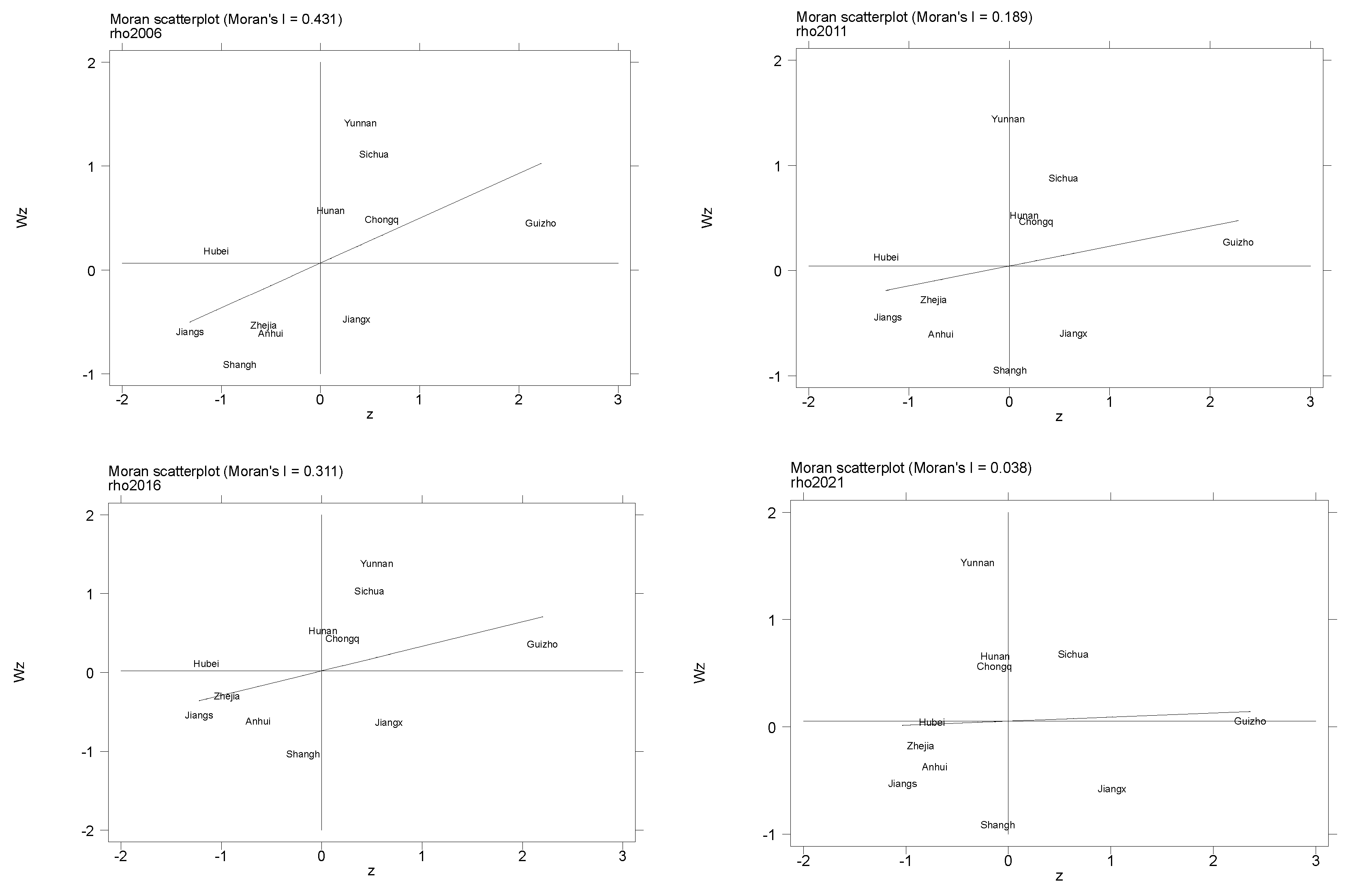
3.1. Changes in Spatial Patterns

Spatial Autocorrelation Test

To determine whether there is a spatial correlation of agricultural surface source pollution in the Yangtze River Economic Belt, we conducted a global spatial autocorrelation test based on geographic neighboring weights for agricultural surface source pollution in this region for the period from 2006 to 2020. As shown in

Table 2. Values of global Moran’s I index for agricultural surface source pollution in provinces and municipalities of the Yangtze River Economic Belt for the period from 2006 to 2020.

Year	I	Year	I
2006	0.431 ***	2014	0.087 **
2007	0.034 ***	2015	0.158 ***
2008	0.017 **	2016	0.311 **
2009	0.271 *	2017	0.023 **
2010	0.176 ***	2018	0.156 ***
2011	0.189 **	2019	0.022 **
2012	0.123 **	2020	0.087 *
2013	0.146 *	2021	0.380 *

Note: *, **, and *** indicate significance at the 10%, 5%, and 1% levels of significance, respectively.

, global Moran’s I index values for the overall agricultural surface source pollution levels in China’s Yangtze River Economic Belt from 2006 to 2020 were all significant at the 10% level, with spatially positive correlations ranging from 0.15 to 0.45. These findings thus indicate that, at the provincial and municipal levels, agricultural surface pollution in the Yangtze River Economic Belt manifests as a spatial aggregation phenomenon that has shown an increasing trend in recent years.

3.2. Spatial Aggregation Characteristics

To further examine the spatial aggregation characteristics of agricultural surface source pollution in the Yangtze River Economic Zone, we used the local Moran I index to assess the aggregation of pollution in the provinces and cities of this region. Moran I scatter plots of agricultural surface source pollution in 2006, 2011, 2016, and 2021 were produced using ArcGIS10.7 software.

3.3. Spatial Correlation Test

As shown in Figure 1, the local Moran indices of agricultural surface pollution in the four years 2006, 2011, 2016, and 2021 were 0.431, 0.189, 0.311, and 0.038, respectively, all of which were significant, thus indicating that agricultural surface pollution in each province was characterized by strong spatial autocorrelation. In the Moran scatter plots, “H-H” (high-high) and “L-L” (low-low) values are located in one or three quadrants, reflecting the positive spatial correlation of environmental pollution; “H-L” (high-low) and “L-H” (low-high) are located in one or three quadrants, reflecting the positive spatial correlation of environmental pollution; “L-H” (low-high) are located in quadrants 2 and 4, reflecting the negative spatial correlation of environmental pollution.

The “H-H” agglomeration pattern of agricultural surface pollution (Figure 1) reflects high environmental pollution areas that are surrounded by high environmental pollution provinces, for which the spatial variability is relatively small. These areas include Yunnan, Guizhou, Sichuan, and the western underdeveloped areas, in which the proportion of primary industries is relatively high. The “L-L” agglomeration pattern of agricultural surface pollution, that is, low environmental pollution areas surrounded by other low environmental pollution provinces, similarly shows relatively little spatial variability. These areas include Jiangsu, Zhejiang, Shanghai, and Anhui, in which tertiary industries account for a high proportion of the developed coastal areas. Overall, the above analysis reveals that there is a significant positive spatial correlation between agricultural surface pollution and China, and a homogeneous spillover effect of agricultural surface pollution is evident. Moreover, this variability could be attributed to differences in the climate and crops cultivated in the assessed regions.

3.4. Analysis of Empirical Results

The analysis described in the previous section revealed that there is a spatial aggregation of agricultural surface pollution in the Yangtze River Economic Belt in China. On the basis of this finding, we constructed a spatial Durbin model to further examine the specific impacts of environmental regulation, input factor market distortion, and labor transfer on the patterns of agricultural surface pollution.

Prior to performing regression analysis, we assessed a spatial econometric model in four steps [36]. Firstly, the LM test based on OLS estimation of the above models rejected the original hypothesis of “no spatial autocorrelation,” thereby indicating that spatial econometric analysis should be conducted. Secondly, Hausman test results were found to be significant at the 5% level, thereby enabling us to reject the random effect and focus on the fixed effect. Thirdly, the LR and Wald test significantly rejected the original hypothesis, indicating that the SDM does not reduce to a spatial error model (SEM) or a spatial lag model (SAR). Finally, the above models were estimated using spatially fixed, time-fixed, and spatiotemporal double-fixed effects. As shown in

Table 3. Estimation results obtained using the spatial a Durbin panel regression model.

Variables	Spatial-Fixed Effects		Time-Fixed Effects		Spatio-Temporal-Fixed Effects
ER/W × ER	−0.167 **	−0.056 *	−1.205 ***	0.087	−0.023 *	−0.377 **
Dis/W × Dis	0.127	0.348 **	2.416 ***	2.007 ***	0.054 **	0.873 ***
LM/W × LM	−0.417 *	−0.947	1.122 ***	−0.320 ***	−0.476 *	−0.151
Lncpi1/W × lncpi1	0.675 **	0.878 ***	1.128 **	0.747	0.234	−1.856 ***
S2/W × s2	−0.979 ***	−0.417 *	−0.219 *	−1.458 ***	−0.764 ***	−0.809 **
t/W × t	0.219	0.476 *	−0.517	0.725 ***	0.151 **	0.513 ***
ρ	−0.219 **		−0.654 ***		−0.135 *
N	176		176		176
R2	0.5471		0.7412		0.5819

Note: *, ** and *** indicate significance at the 10%, 5%, and 1% levels of significance, respectively.

, the results indicated that the SDM under time-fixed effects has a higher degree of fit and the largest R² value, thereby indicating that it is more appropriate to select the time-fixed SDM. Consequently, for analysis in this study, we selected the spatial Durbin model under time-fixed effects.

3.4.1. Spatial Durbin Models

Panel spatial econometric models are mainly categorized into three types: SAR, SEM, and SDM; with respect to robustness, the results obtained using these models under static time-fixed effects are also reported here, as shown in

Table 4. Static spatial panel model econometric regression results.

Variables	SDM		SAR	SEM
ER/W × ER	−0.674 ***	−0.014 **	−0.456 ***	−0.352 **
Dis/W × Dis	1.766 ***	2.980 ***	2.433 ***	1.098 ***
LM/W × LM	−0.734 ***	−0.675 ***	−0.546 ***	0.489 ***
Lncpi1/W × lncpi1	1.218 **	1.657 *	0.452 ***	0.082
S2/W × s2	−0.356 *	−1.209 ***	−0.561 *	−0.144
t/W × t	0.597 **	1.615 ***	0.462 ***	−0.407
ρ	−0.764 ***		−0.143 ***	−0.105 *
N	176		176	176
R2	−0.674 ***		−0.014 **	−0.456 ***

Note: *, ** and *** indicate significance at the 10%, 5%, and 1% levels of significance, respectively.

.

As can be seen from the regression results presented in Table 4, the sign of the regression coefficients of the variables in each model and the size of the values are essentially consistent, indicating that the results are robust and credible. Among these, the time-fixed spatial Durbin model has the largest decidable coefficient, which indicates that the model selected in this study is more applicable.

Agricultural surface pollution. The coefficient ρ in the spatial Durbin model was found to be significantly negative at the 1% level, thereby indicating that agricultural surface pollution between neighboring provinces is characterized by a “neighbor-as-neighbor” effect; that is, local pollution has a negative spatial spillover effect on the pollution in neighboring provinces, and an intensification of local pollution will reduce the pollution of neighboring provinces.

Influence of environmental regulations on agricultural surface pollution. The coefficients of environmental regulation for each of the assessed models were found to be significantly negative, thereby indicating that environmental regulation is an important approach for suppressing agricultural surface pollution. We suspect that this effect could be attributable to the fact that when governments increase the amount of investment in environmental protection or promote the implementation of ecological compensation policies, enterprises will have more funds to improve their production processes to levels that are perceived to be “environmentally friendly,” thereby reducing the emission of pollutants.

The influence of factor market distortion on agricultural surface pollution. We found that in each of the assessed models, the coefficients of factor market distortion were significantly positive, thus indicating that an increase in factor market distortion has the effect of exacerbating agricultural surface pollution. This effect could be attributable to the fact that the greater the degree of distortion in the fertilizer market, the greater the circulation of low-priced inferior-quality fertilizers in the market, and the massive use of poor-quality fertilizers will further exacerbate agricultural surface pollution.

We subsequently examined the effects of factor market distortion on agricultural surface pollution in neighboring provinces and cities. The coefficient of W × Dis in Table 3 was found to be significantly positive, thus indicating that factor market distortion has a strong spatial spillover effect. With the rapid development of the network, information barriers are broken, and when the fertilizer market in a province is distorted to a considerable extent, farmers in adjacent provinces are more willing to purchase low-priced fertilizers from such provinces, which indirectly exacerbates agricultural surface pollution in the adjacent provinces.

Impact of labor transfer on agricultural surface pollution. Using each of the assessed models, the coefficients of labor transfer were found to be significantly negative, thereby indicating that an increase in the proportion of labor force transfer exacerbates the degree of agricultural surface source pollution. As a consequence of the transfer of the rural labor force, farmers may increase the application of fertilizer to compensate for the loss of income associated with this portion of the labor force, which in turn exacerbates agricultural surface pollution.

Influence of control variables. The regression coefficients of the village consumer price index and industrial structure were both shown to be significantly positive, thus indicating that an increase in the consumer price index of rural residents and the gradual shift of the industrial structure to secondary industries will exacerbate agricultural surface pollution to a certain extent. The regression coefficient of science and technology level is significantly negative, indicating that scientific and technological progress will alleviate agricultural surface pollution to some extent.

3.4.2. Effect Decomposition Measures

Given that the variables of the SDM model are characterized by spatial lag terms, the direction and significance of the coefficients of the lag terms are still valid. However, the values do not directly reflect the influence of the independent variables on the dependent variable. Therefore, it is necessary to further apply partial differentiation to decompose the spatial spillover effects into direct, indirect, and total effects. In this study, effect decomposition was carried out on the basis of the SDM model, in which the direct effect represents the impact of environmental regulation intensity, the degree of distortion of the fertilizer factor market, and the transfer of the labor force on agricultural surface pollution in a given province. Similarly, the spatial effect in a given province represents the impact of environmental regulation intensity, the degree of fertilizer factor market distortion, and labor force transfer on agricultural surface pollution in neighboring provinces.

As shown in

Table 5. The decomposition of spatial effects.

Variables	Decomposition of Effects
	Direct Effect	Spatial Effect	Total Effect
ER	−0.134 ***	−0.145	0.102
Dis	1.203 ***	1.403 ***	2.145 ***
LM	0.346 ***	−0.207	0.203 ***
lncpi	2.103 **	1.245	2.301
S2	0.807 ***	1.093 ***	−1.128 ***
t	−0.163	1.018 ***	0.217 **

Note: ** and *** indicate significance at the 5%, and 1% levels of significance levels, respectively.

, in the case of direct effects, the impact of environmental regulation on agricultural surface pollution in the Yangtze River Economic Zone is significantly negative, thereby indicating that the greater the intensity of environmental regulation in a province, the greater the extent to which agricultural surface pollution status can be significantly improved. The impact of the degree of factor market distortion and the transfer of labor in a province is significantly positive, thus indicating that reductions in the degree of fertilizer factor market distortion and the number of labor transfers can effectively contribute to reducing the sources of agricultural surface pollution. With respect to the spatial effect, the degree of factor market distortion was established to have a significant spatial effect on agricultural surface pollution in the Yangtze River Economic Zone, and there is an obvious spillover effect. In contrast, we found the spatial effects of environmental regulation and labor force transfer to be non-significant, thus indicating that spatial effects have a smaller impact on agricultural surface pollution in neighboring provinces and cities and that there is no clear-cut spillover effect. Among the total effects, the degrees of factor market distortion and labor transfer were found to have more significant effects on agricultural surface pollution.

3.4.3. Robustness Test

Although the aforementioned estimation results obtained using the spatial Durbin model revealed the effects of environmental regulation, factor market distortion, and labor transfer on agricultural surface pollution, to compensate for the lack of static spatial measurement, and simultaneously perform an analysis of the robustness of our regression results, we introduced the lagged term of agricultural surface pollution as an explanatory variable, and performed regression using the systematic GMM method.

The results obtained by applying the Hausman test revealed that fixed effects were more relevant than random effects, and on the basis of an AR (2) value greater than 0.1 in the autocorrelation test, we were unable to reject the original hypothesis that the random perturbation term had no autocorrelation. Furthermore, the value obtained for the Sargan over-identification test was found to be greater than 0.1, again indicating the probable veracity of the original hypothesis; that is, all instrumental variables are exogenous and valid.

The regression results presented in

Table 6. Robustness test.

Variables	Dynamic GMM
L1	0.7609 ***
ER	−0.0356 ***
D	0.1450 **
LM	−0.5512 ***
CPI	0.6770 *
S	−0.1026 **
T	0.0145 **
AR (1)	−0.92
AR (2)	−0.78
Sargan	138
N	176

Note: *, ** and *** indicate significance at the 10%, 5%, and 1% levels of significance, respectively.

are consistent with the regression results obtained using the spatial Durbin model under time fixation, and the robustness was assessed. As the coefficients and levels of significance of the control variables estimated using the systematic GMM method are similar to those of the static panel, they are not presented here.

3.4.4. Threshold Effects

(1)

Threshold effects

To further analyze the non-linear role of factor market distortion on agricultural surface pollution under the influence of environmental regulation, we applied Hansen’s panel threshold model, which adopts environmental regulation as the threshold variable and incorporates labor transfer into the control variables to facilitate assessments of the threshold effect. The results (presented in

Table 7. Threshold number test and threshold estimation results.

Threshold Number	F-Statistic	p-Value	Critical Value			Threshold	95% Confidence Interval
			1%	5%	10%
Single Threshold	10.12	0.0102	6.2475	8.5790	11.8042	η1 = 0.1405	(0.0801, 0.0867)
Double threshold	1.74	0.2023	7.9022	11.3527	16.2680

) show that, whereas the results of the single threshold test were significant, those of the double threshold test did not reach the level of significance, thereby indicating that there is only a single threshold value. Accordingly, a single threshold model should be used to analyze factor market distortion and agricultural surface pollution.

(2)

Analysis of the threshold regression results

As shown in

Table 8. Coefficient estimation results of threshold and linear models.

Variables	Estimated Value
D (D ≤ 0.1405)	0. 4572 **(3.07)
D (D > 0.1405)	0.2013 * (3.04)
LM	0.1178 * (1.85)
CPI	0.2147 ** (2.60)
S	−0.7304 *** (−4.50)
T	0.1217 ** (2.48)
conr	4.8301 *** (12.32)
R2	0.975

Note: *, ** and *** indicate significance at the 10%, 5%, and 1%levels of significance, respectively.

, when environmental regulation is lower or greater than the first threshold, factor market distortions significantly exacerbate agricultural surface pollution. However, the effect of enhanced pollution is characterized by a non-linear pattern of an initial increase and subsequent decline. We speculate that this pattern could be attributable to the fact that when the intensity of environmental regulation is low, farmers tend to economize by using inferior quality fertilizers, which, accordingly, has the effects of enhancing agricultural surface pollution. Conversely, with an increase in the intensity of environmental regulations, the compensatory benefits gained by farmers from using organic fertilizers are greater than the costs saved by using poor-quality fertilizers, and farmers tend to use organic fertilizers, which in turn mitigates the rate of increase in agricultural surface pollution.

4. Conclusions and Recommendations

In this study, we demonstrated that there is a positive spatial correlation between agricultural surface pollution in the Yangtze River Economic Belt and an obvious homogeneous spillover effect. Our analysis of the contributory factors revealed that an increase in the distortion of input factor markets will promote a significant increase in agricultural surface pollution within the Yangtze River Economic Zone, whereas increases in governmental environmental regulation and the numbers of rural laborers migrating from the country to urban areas will significantly reduce the agricultural surface pollution in this region. Further research indicated that factor market distortion has a significant single-threshold effect on the effects of environmental regulation on agricultural surface pollution and that this effect is characterized by a non-linear pattern of an initial increase and subsequent decline.

Based on our findings in this study, we propose the following policy recommendations.

Firstly, from the perspective of the coordinated regional development of the Yangtze River Economic Belt, given the tendency of spatial agglomeration of agricultural surface pollution, the mutual influence between different provinces and municipalities has become an important factor in determining the level of regional agricultural surface pollution. Provincial and municipal governments in the Yangtze River Economic Belt region should accordingly strengthen the linkage and establish a sound system of common governance, not only to formulate feasible governance programs in their provinces and municipalities according to local conditions, but also to take into consideration the governance links with their neighboring provinces and the municipalities therein. In particular, the western provinces and municipalities, which tend to be characterized by the highest levels of pollution in the economic zone, should break away from the original “who pollutes, who governs” mode and examine their common governance systems. The government can also refer to the legal enactment framework in the United States, i.e., through the central government, to issue a general overview of the general direction, and each local government to enact locally adapted laws and policies according to the environmental pollution situation in each place.

Secondly, when governments formulate environmental regulations, they can appropriately increase the strength of regulations and continuously improve their applicability and feasibility. Moreover, attention should be paid to environmental regulations and other policies to coordinate operations, such as market mechanisms that match the degree of perfection, thereby enabling the identification of the maximum extent of agricultural pollution that can alleviate the degree of surface pollution of the “first threshold value”. In addition, to implement ecological compensation incentives, governments should not only balance rewards, such as in the simultaneous formulation of punitive laws and regulations, but also continue to improve the agricultural ecological protection compensation system in the system-level design of ecological compensation mechanisms, fertilizer reduction, soil transformation, and the use of green production technology by farmers.

Thirdly, the effective supervision of all aspects of the production and marketing of green agricultural products can be achieved by constructing a model of co-management and co-regulation between the state and society. Taking the fertilizer factor market as an example, governments could promote a balance between supply and demand in the fertilizer market by limiting the minimum or maximum price of fertilizers and granting tax incentives or subsidies, thereby reducing the circulation of low-quality fertilizers and the intensity of fertilizer application to a certain extent.

Fourthly, manpower is an effective guarantee for promoting rural revitalization. If a country wishes to strengthen and promote agriculture, it should focus on cultivating talent. Accordingly, local governments should implement policies designed to attract and cultivate high-quality farmers. In addition, in terms of policy, governments should optimize rural policies, thereby providing incentives for urban migrant workers and unemployed college students to return to their hometowns to start their businesses. Similarly, in terms of education, relevant programs should be developed to cultivate agricultural professionals, whilst promoting the teaching of the concept of sustainable agricultural development. In terms of industry, the resources of the Internet should be exploited to achieve the development of industrial wisdom, promote the progress of human resources, and create a cultured skilled workforce with a good theoretical and practical understanding of the treatment of pollution. The “three farmers” team.

Finally, our study only examined the factors affecting agricultural surface pollution in the Yangtze River Economic Zone and did not examine the effects of agricultural surface pollution on other factors such as regional economic development, ecological environment, water quality, and groundwater. Meanwhile, for the specific content of agricultural surface pollution, only its main components, including total Tn, Tp, and Cod, were studied, ignoring some very trace but difficult-to-handle heavy metals, including boron, potassium, and selenium, which enter the soil through fertilizers and pesticides, and need to be solved through the control of fertilizers and remediation [43]. In the future, we plan to broaden our research to cover these aforementioned areas.

References

1. China’s Import and Export of Agricultural Products, January–December 2022. Available online: http://www.moa.gov.cn/ztzl/nybrl/rlxx/202301/t20230128_6419275.htm (accessed on 20 July 2023).
2. Xia, Q.; Li, D.; Zhou, H. Research on the impact of farm household part-time employment on agricultural surface pollution. China Popul.-Resour. Environ. 2018, 131–138. [Google Scholar]
3. Zhang, Y.; Yang, L.; Ouyang, H.; Song, L. Paths for improving agricultural green production efficiency in the Yangtze River Economic Belt based on surface source pollution and carbon emission. Water Resour. Econ. 2022, 40, 24–33+41+94. [Google Scholar]
4. Chai, Y.; Jiang, L. The gaming behavior and dilemma resolution of participating subjects in China’s agricultural low-carbon development. Rural Econ. 2013, 8–12. [Google Scholar]
5. Huang, Z.; Zhong, Y.; Wang, X. Impacts of different policies on pesticide application behavior of farm households. China Popul.-Resour. Environ. 2016, 26, 148–155. [Google Scholar]
6. Ma, J.; Dan Zeng, W.; Gao, H. Analysis of the spatiotemporal characteristics and impacts of planting industry agglomeration and agricultural non-point source pollution: Evidence from the Yangtze River Basin. Resour. Ind. 2023, 1–19. [Google Scholar] [CrossRef]
7. Ministry of Ecology and Environment of the People’s Republic of China; National Bureau of Statistics of the People’s Republic of China; Ministry of Agriculture and Rural Development of the People’s Republic of China. Announcement on the Release of the Second National Pollution Source Census Bulletin. Available online: https://www.mee.gov.cn/xxgk2018/xxgk/xxgk01/202006/t20200610_783547.html (accessed on 9 June 2020).
8. Hao, G.; Xiong, X.; Zhao, Y.; Fan, H.; Xu, L. Evaluation of water quality of Luanhe River tributaries and correlation between sources of agricultural surface pollution. Water Sav. Irrig. 2023, 59–69. [Google Scholar]
9. Wang, S.; Yang, D.; Sun, J.; Tang, L.; Wang, P.; Lu, S. Current situation and characterization of agricultural surface pollution in China. Water Resour. Conserv. 2021, 37, 140–147+172. [Google Scholar] [CrossRef]
10. Li, B.; Ma, H.; Long, J. A review of environmental federalism theory. Financ. Trade Econ. 2009, 131–135. [Google Scholar] [CrossRef]
11. Dasgupta, S.; Laplante, B.; Mamingi, N.; Wang, H. Inspections, Pollution Prices, and Environmental Performance: Evidence from China. Ecol. Ecol. Econ. 2001, 36, 487–498. [Google Scholar] [CrossRef]
12. Thiel, C.; Nijs, W.; Smoes, S.; Schmidt, J.; van Zyl, A.; Schmid, E. The impact of the EU Car CO2 Regulation on the Energy System and the Role of Electro-mobility to Achieve Transport Decarbonisation. Energy Policy 2016, 96, 153–166. [Google Scholar] [CrossRef]
13. Elgin, C.; Mazhar, U. Environmental Regulation, Pollution and the Informal Economy; Working Papers of Bogazic University: Istanbul, Turkey, 2012. [Google Scholar]
14. Ma, J.; Yang, C.; Cui, H.-Y.; Wang, X. Environmental effects and impact mechanisms of agricultural insurance—An examination from the perspective of chemical fertilizer surface pollution in China. Insur. Res. 2021, 46–61. [Google Scholar] [CrossRef]
15. Wu, C.; Gao, K. Research on environmental regulation and environmental efficiency of high-tech manufacturing industry in the Yangtze River Economic Belt—The test based on “Porter’s hypothesis”. Yangtze River Basin Resour. Environ. 2022, 31, 972–982. [Google Scholar]
16. Cao, L.; Ruan, C.; Lei, T. EKC test of agricultural surface source pollution in coastal areas of China analysis based on spatial Durbin model. Jiangsu Agric. Sci. 2021, 49, 239–245. [Google Scholar]
17. Ge, J.; Zhou, S. Whether factor market distortion stimulates agricultural surface pollution—Take chemical fertilizer as an example. Agric. Econ. Issues 2012, 33, 92–98+112. [Google Scholar]
18. Zhang, S.; Ebenstein, A.; McMillan, M.; Chen, Z. Rural labor migration, fertilizer overuse and environmental pollution. Comp. Econ. Soc. Syst. 2017, 149–160. [Google Scholar]
19. Luan, J.; Li, T.; Ma, K. Research on the impact of labor transfer on agricultural fertilizer surface pollution in China. World Agric. 2016, 63–69+199. [Google Scholar] [CrossRef]
20. He, Z.; Cao, C.; Wang, J. Spatial spillover research on environmental regulation, industrial agglomeration and environmental pollution. East China Econ. Manag. 2022, 36, 12–23. [Google Scholar]
21. Dong, X.L.; Zhang, Y.Y. Industrial Division of Labor, Environmental Pollution and Regional Economic Development—Empirical Evidence Based on Heavy Chemical Industry in the Yangtze River Economic Belt. Econ. Jingwei 2020, 37, 20–28. [Google Scholar]
22. Ran, Q.-Y.; Xu, L.-N. Environmental regulation, interprovincial industrial transfer and pollution spillover effects—Based on the spatial Durbin model and dynamic threshold panel model. East China Econ. Manag. 2019, 33, 5–13. [Google Scholar]
23. Hansen, B.E. Threshold effects in non-dynamic panels: Estimation, testing and inference. J. Econom. 1999, 93, 345–368. [Google Scholar] [CrossRef]
24. Lai, S.-Y.; Du, P.-F.; Chen, J.-N. A non-point source pollution survey and assessment method based on unit analysis. J. Tsinghua Univ. (Nat. Sci. Ed.) 2004, 1184–1187. [Google Scholar]
25. Chen, M.; Chen, J.; Lai, S. Inventory analysis and spatial characteristics of agricultural and rural pollution in China. China Environ. Sci. 2006, 751–755. [Google Scholar]
26. Ma, J.; Gao, H.; Shi, Y.Q. Study on the quantification and spatial and temporal pattern of carbon offset in the Yangtze River Economic Belt. Resour. Ind. 2023, 25, 52–64. [Google Scholar] [CrossRef]
27. Qin, T.; Peng, J.; Dang, Z.; Wang, J. Impact of environmental decentralization and environmental regulation on agricultural surface pollution. China Popul.-Resour. Environ. 2021, 31, 61–70. [Google Scholar]
28. Zhan, J.; Xu, Y. Environmental regulation, agricultural green productivity and food security. China Popul.-Resour. Environ. 2019, 29, 167–176. [Google Scholar]
29. Christensen, L.R.; Jorgenson, D.W.; Lau, L.J. Transcendental Logarithmic Production Frontiers. Rev. Econ. Stat. 1973, 55, 28–45. [Google Scholar] [CrossRef]
30. Shi, J.; Zhao, Z. Ownership constraints and factor price distortions—An empirical analysis based on Chinese industrial sector data. Stat. Res. 2007, 42–47. [Google Scholar] [CrossRef]
31. Li, X.; Lu, Z. Evaluation of Innovation Factor Allocation Efficiency in the Pearl River Delta Region-Analysis Based on beyond Logarithmic Production Function. Reform 2021, 97–111. [Google Scholar]
32. Liu, L.; Liu, J. Analysis of the elasticity of substitution between organic fertilizer and chemical fertilizer based on beyond logarithmic production function—From a survey on the fertilizer application behavior of fruit farmers in the main apple-producing areas of Bohai Bay. Agric. Technol. Econ. 2022, 69–82. [Google Scholar] [CrossRef]
33. Liu, P.; Luo, C. Labor marginal output and firm wage distribution. Econ. Dyn. 2019, 52–65. [Google Scholar]
34. Gu, R. Research on the Impact of Labor Wage Distortion on Enterprise Innovation and Its Role Mechanism. Ph.D. Thesis, Chongqing University, Chongqing, China, 2020. [Google Scholar]
35. Shi, H.-P.; Yi, M.-L. Environmental regulation, non-agricultural part-time employment and agricultural surface source pollution—An example of chemical fertilizer application. Rural. Econ. 2020, 127–136. [Google Scholar]
36. Ma, J.; Le, Z. Analysis of spatial differences and influencing factors of agricultural surface pollution in China. Agric. Mod. Res. 2021, 42, 1137–1145. [Google Scholar]
37. Ma, J.; Cao, F.; Zhou, P. Analysis of the evolution of eco-efficiency and driving factors of cities in the Yangtze River Economic Belt. Resour. Ind. 2020, 22, 32–40. [Google Scholar]
38. China Rural Statistics Yearbook. Available online: https://www.shujuku.org/china-rural-statistical-yearbook.html (accessed on 20 July 2023).
39. China Environmental Statistics Yearbook. Available online: http://navi-cnki-net-s.vpn.hhu.edu.cn:8118/knavi/yearbooks/YHJSD/detail?uniplatform=NZKPT&language=chs (accessed on 20 July 2023).
40. China Statistical Yearbook. Available online: http://www.stats.gov.cn/sj/ndsj/ (accessed on 20 July 2023).
41. National Compendium of Cost-Benefit Information on Agricultural Products. Available online: https://www.shujuku.org/agricultural-products-cost-benefit.html (accessed on 20 July 2023).
42. China Science and Technology Statistical Yearbook. Available online: http://navi-cnki-net-s.vpn.hhu.edu.cn:8118/knavi/yearbooks/YBVCX/detail?uniplatform=NZKPT (accessed on 20 July 2023).
43. Yin, A.; Shen, C.; Huang, Y.; Yue, M.; Huang, B.; Xin, J. Reduction of Cd accumulation in Se-biofortified rice by using fermented manure and fly ash. Environ. Sci. Pollut. Res. 2020, 27, 39391–39401. [Google Scholar] [CrossRef] [PubMed]
Figure 1. Localized Moran scatterplots for agricultural surface source pollution in the Yangtze River Economic Zone for the years 2006, 2011, 2016, and 2021.
Sustainability 15 14753 g001