Abstract
Pavement deterioration models provide the basis for predicting future changes in network conditions, estimating future funding needs, and determining the effectiveness and timing of maintenance and rehabilitation activities. Determining the accurate structural condition of pavements helps identify effective maintenance strategies which enhance the sustainability and service life of pavements. This study aimed to use the Traffic Speed Deflectometer (TSD) and Fast Falling Weight Deflectometer (FFWD) for project-level evaluation of pavements and use pavement properties to calibrate current models that help to predict the structural condition of pavements. Model parameters were calibrated to determine the effective structural number and tensile strains at the bottom of asphalt concrete for asphalt and composite pavements from TSD deflections. Tensile strains from the KENLAYER highlighted varied behaviors for composite pavements. A significant improvement in the calibration was observed for asphalt concrete pavements. While the TSD has higher daily operational costs than FWD, its per-mile cost is significantly lower, making it a viable choice for extensive coverage, even though the quantitative results might differ between the two devices.
1. Introduction
Transportation, specifically highway infrastructure, plays a crucial role in the socioeconomic development of a country. Over the last few decades, the United States (U.S.) has invested heavily in developing its highway infrastructure network. As the infrastructure systems are reaching a mature state, the state transportation agencies are changing their focus from constructing new highways to maintaining the existing ones to meet minimum performance requirements required by the Federal Highway Administration (FHWA) for federal funding. In 2017, over USD 80 billion was spent only to operate, maintain, and rehabilitate the U.S. highway infrastructure [1]. However, the rapid deterioration of the highway infrastructure and limited resources at transportation agencies have necessitated the need for incorporating technically appropriate maintenance solutions that are economically viable and environmentally sustainable. Therefore, there is a need for a well-equipped Pavement Management System (PMS) to provide decision-makers with the required information to ensure efficient and sustainable management of highways.
Transportation agencies collect pavement health or condition data and populate the PMS to optimize agency resources for pavement maintenance and rehabilitation needs. Generally, a PMS uses condition indices or scores of roadway pavements at different levels. The American Association of State Highway and Transportation Officials (AASHTO) defines PMS as “a set of tools or methods that assist decision-makers in finding optimum strategies for providing, evaluating, and maintaining pavements in a serviceable condition over a period of time” [2]. The PMS helps with the decision making for long-term “needs-based” budgeting at the network level to handle the overall state of the network. At the project level, PMS covers the most economical methods of maintenance and rehabilitation for each road segment. Several Maintenance, Rehabilitation, and Reconstruction (MRR) strategies have been proposed in different studies for project-level assessment [3,4,5,6]. Allocating limited resources in the most effective way possible to maximize benefits during the asset life cycle is a crucial component of asset management.
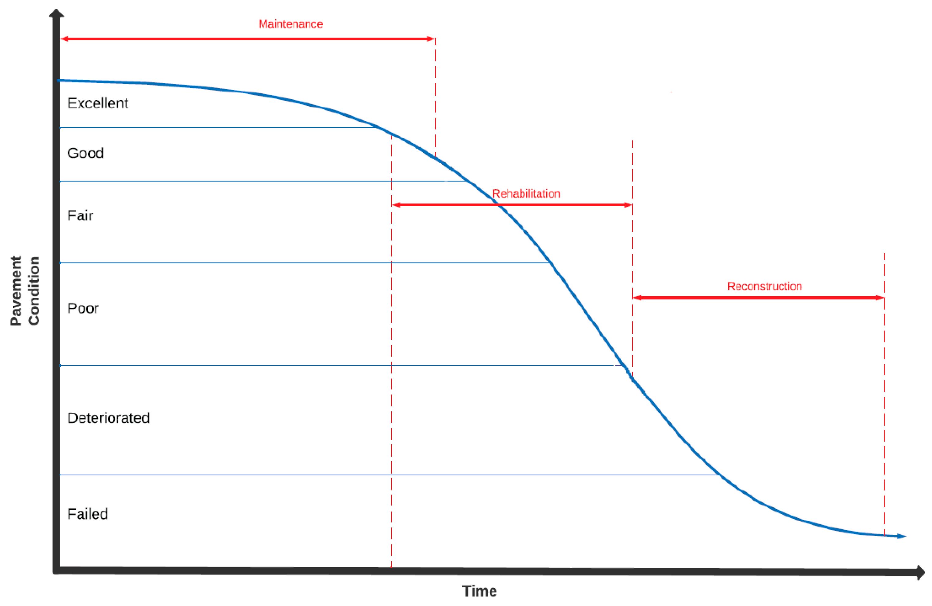
Roadway pavement condition data involve structural conditions (e.g., structural number, layer modulus, and drainage) as well as surface conditions (e.g., roughness, rut, crack, and patch) and other factors (e.g., safety, traffic, and accidents) to determine the condition or rating of the pavement. The structural condition of pavements plays an important role in the project-level PMS. The structural capacity is an indicator of the remaining service life and the condition of the pavements. Pavement performance can go down significantly, and the resulting maintenance and rehabilitation cost can increase exponentially with time, as shown in Figure 1.
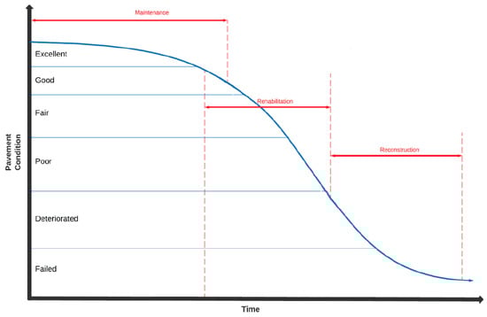
Figure 1.
Condition of pavement over time.
Destructive and non-destructive methods are used to assess the condition of pavements at the project level. The Falling Weight Deflectometer (FWD) and Fast Falling Weight Deflectometer (FFWD) are tools that are commonly used in a PMS at project level. Since the 1980s, the FWD has been one of the most widely used devices for pavement condition assessment in the U.S. In this test, a deflection basin is measured under an impact load using geophones or force balance seismometers [7]. The size of the plate and impact load depends on the material being tested (asphalt, stabilized subgrade, compacted subgrade, etc.). Generally, an impact load is applied on a circular plate 12 in. (300 mm) in diameter and placed on the surface of the pavement. Deflections at the center of the load as well as 12 in. (300 mm), 24 in. (600 mm), 36 in. (900 mm), 48 in. (1200 mm), 60 in. (1500 mm), and 72 in. (1800 mm) from the center of the plate are collected with a FWD.
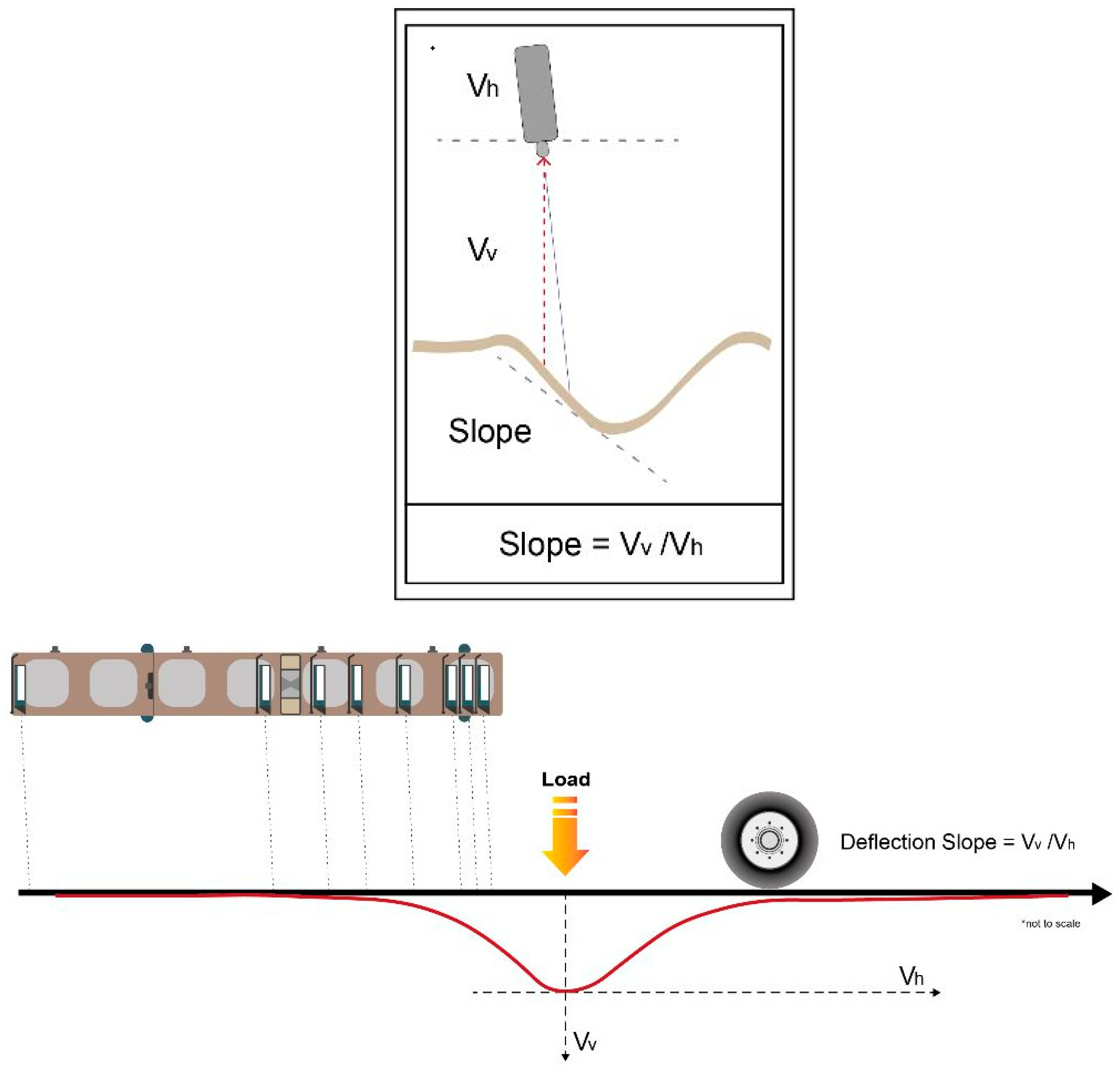
Recently, the Traffic Speed Deflectometer (TSD) has emerged as a useful tool for measuring surface deflections of pavements at close intervals as well as roughness, texture, and rut at traffic speed. The TSD is an instrumented truck that applies a rear axle load varying from 13 to 28 kips (57 kN to 125 kN) on the pavement and measures deflections. It commonly has seven Doppler laser sensors that are positioned at 0, 8 in. (200 mm), 12 in. (300 mm), 24 in. (600 mm), 36 in. (900 mm), 48 in. (1500 mm), 60 in. (1800 mm) and 72 in. (2100 mm) in front of the loaded axle (i.e., traffic direction) and a single laser located outside the bowl that serves as the reference sensor [8]. The TSD can operate at different speeds, although 60 mph (96.5 km/h) with a data collection rate of 1 KHz is commonly used [8]. The TSD determines the deflection slope from the vertical pavement deflection velocity and the vehicle horizontal velocity for each location of laser sensor. From these data, a deflection basin is defined and used to represent the profile of the deflected pavement. Pavement deflection is obtained from the deflection slope by integration. Figure 2 shows a pictorial view of the TSD data collection approach. Additional details on the TSD can be found elsewhere [8,9,10,11,12,13]. As data are collected at traffic speed, no traffic control is needed. The TSD is gaining popularity within transportation agencies for pavement condition assessment and management at the network level.
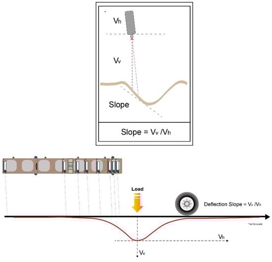
Figure 2.
Deflection slope from Traffic Speed Deflectometer [8].
The main differences between the FWD and TSD measurements are the nature of loading (impact load in the FWD and moving half-axle load in the TSD) and measuring sensors (geophones in the FWD and Doppler laser in the TSD). In addition, multiple drops are used in FWD testing that allows verification of the repeatability, while TSD data are collected at close intervals as the instrumented truck moves at traffic speed. One can argue that some accuracy is lost in the TSD due to the averaging process and the approach used in defining the pavement deflection basin. No such issues exist with FWD testing. In addition, the tensors for stress and strain rotate during data collection in the TSD and they remain constant for the FWD. Also, other factors, namely damping, tire pressure, and truck dynamics, can influence TSD data [14].
Despite the advantages of using the TSD in quantifying both surface and structural conditions of roadway pavements, there are issues pertaining to using deflection data in determining tensile strain at the bottom of asphalt concrete (AC) layers and assessing structural capacity or remaining service life of the pavement. The effective structural number (SNeff) and the tensile strain at the bottom of the AC are indicators of the remaining service life of the pavement and the damage induced in the pavement by traffic loading. An accurate estimation of the SNeff and tensile strain at the bottom of the AC can help to characterize the condition of pavements with more certainty and potentially detect deficiencies that can lead to a faster deterioration of the pavement and a higher maintenance cost in future.
Currently, there are several approaches to determine the SNeff and tensile strains at the bottom of AC, from the FWD, modeling or other non-destructive methods [15,16,17,18,19,20]. For example, Rhode proposed a model and estimated necessary values for coefficients to calculate SNeff from FWD deflections and thicknesses of AC [20]. Based on Rhode’s work, Nasimifar proposed new coefficients to estimate SNeff from TSD deflections [21]. Also, AASHTO proposed a method to calculate SNeff from given layer coefficients that are related to the elastic moduli and thicknesses of the pavement layers [2]. Rada et al. proposed a model to estimate tensile strains at the bottom of AC for different layer thicknesses from basin indices that can be calculated from TSD deflections [13].
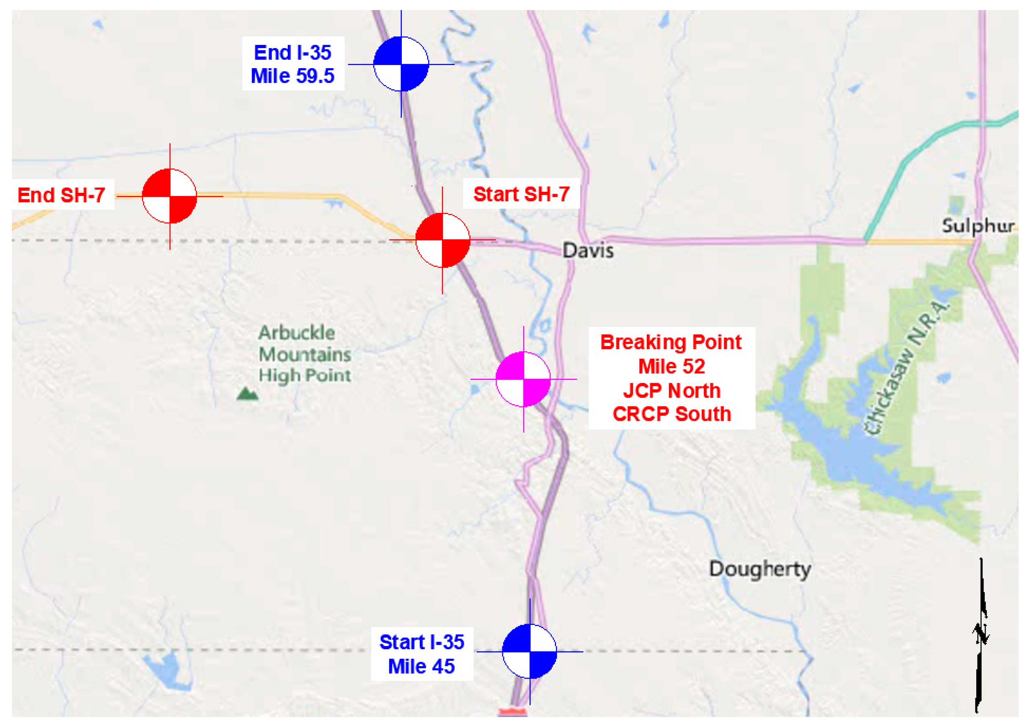
The main objective of this study was to review, compare, analyze, and model the TSD data from Interstate 35 (I-35) and State Highway 7 (SH-7) pavement sections that were collected as a part of a pooled fund study (TPF-5 (385), Pavement Structural Evaluation with Traffic Speed Deflection Devices), conducted by the Virginia Tech Transportation Institute (VTTI). TSD data were collected from several miles of pavement on I-35 and SH-7 in Oklahoma. Specifically, a 14.5-mile segment of I-35 pavement that began at the Carter/Murray County line Mile Post 45 (34.376384, −97.144182) and extended north to Mile Post 59.5 (34.559871, −97.193138) was studied. The SH-7 pavement section started 1 mile west of the intersection with I-35 (34.510042, −97.194876) and extended 5 miles west (34.521343, −97.284874) in Garvin County. Also, FWD data were collected on the same sections of I-35 and SH-7.
In this study, TSD and FWD data were analyzed and compared using statistical and traditional regression methods. The KENLAYER software [18] was used to calculate the deflections, strains, and stresses for the asphalt concrete pavements of SH-7 and composite pavements of I-35. The parameters or coefficients of models proposed by Rada et al. [13], AASHTO [2], and Rhode [20] were calibrated by comparing the TSD and FWD data with KENLAYER outputs. As noted above, a sustainable pavement management plan can only be realized from the true understanding of the conditions of the pavements. An understanding of SNeff and tensile strains at the bottom of AC can lead to a better estimation of the remaining service life of the pavements and improved maintenance, repair, and rehabilitation decisions.
2. Methodologies
In this study, the pavement conditions of a 14.5-mile section of I-35 and a 5-mile section of SH-7 were studied. Figure 3 shows a satellite view of the studied I-35 and SH-7 sections. Based on previous plans, the I-35 section had several modifications over the years. Two different pavement types were observed in the I-35 sections. The section south of Mile Post 52 consisted of an 8- to 10-inch-thick asphalt layer supported by an 8-inch-thick Continuously Reinforced Concrete Pavement (CRCP). The section north of Mile Post 52 had an 8- to 10-inch-thick asphalt layer over a 9-inch-thick Jointed Concrete Pavement (JCP). The SH-7 section consisted of 17 to 21 inches of asphalt with fabric at 1.5 inches below the surface. Layer thicknesses were determined using a Ground Penetration Radar (GPR) and coring.
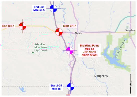
Figure 3.
Satellite view of State Highway 7 and Interstate 35 sections.
A TSD with nine Doppler laser sensors was used for collecting pavement condition data with the help of Australian Road Research Board (ARRB) Systems. The vertical pavement deflection velocities and the vehicle horizontal velocities were recorded at 0 in., 8 in. (200 mm), 12 in. (300 mm), 18 in. (450 mm), 24 in. (600 mm), 36 in. (900 mm), 48 in. (1200 mm), 60 in. (1500 mm), and 72 in. (1800 mm) from the center of the wheel load. Deflections were calculated using the area under the curve (AUTC) model by numerically integrating the deflection bowl. It was observed that the deflection readings of several stations on I-35 section were not recorded by the TSD. Minimal deflection reading, laser reading error, and/or high speed of the TSD may have been responsible for this issue [10,22].
2.1. KENLAYER Analysis
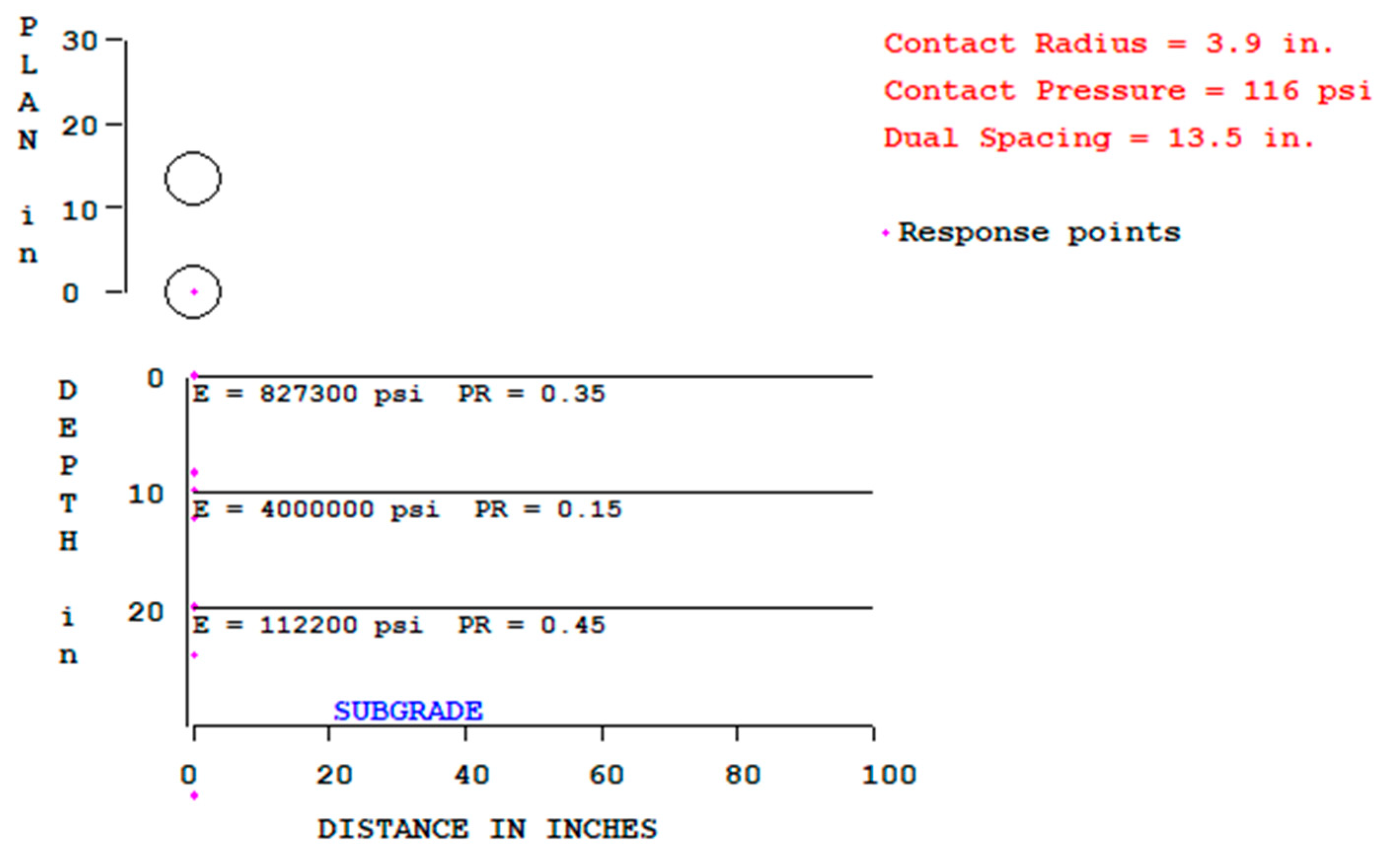
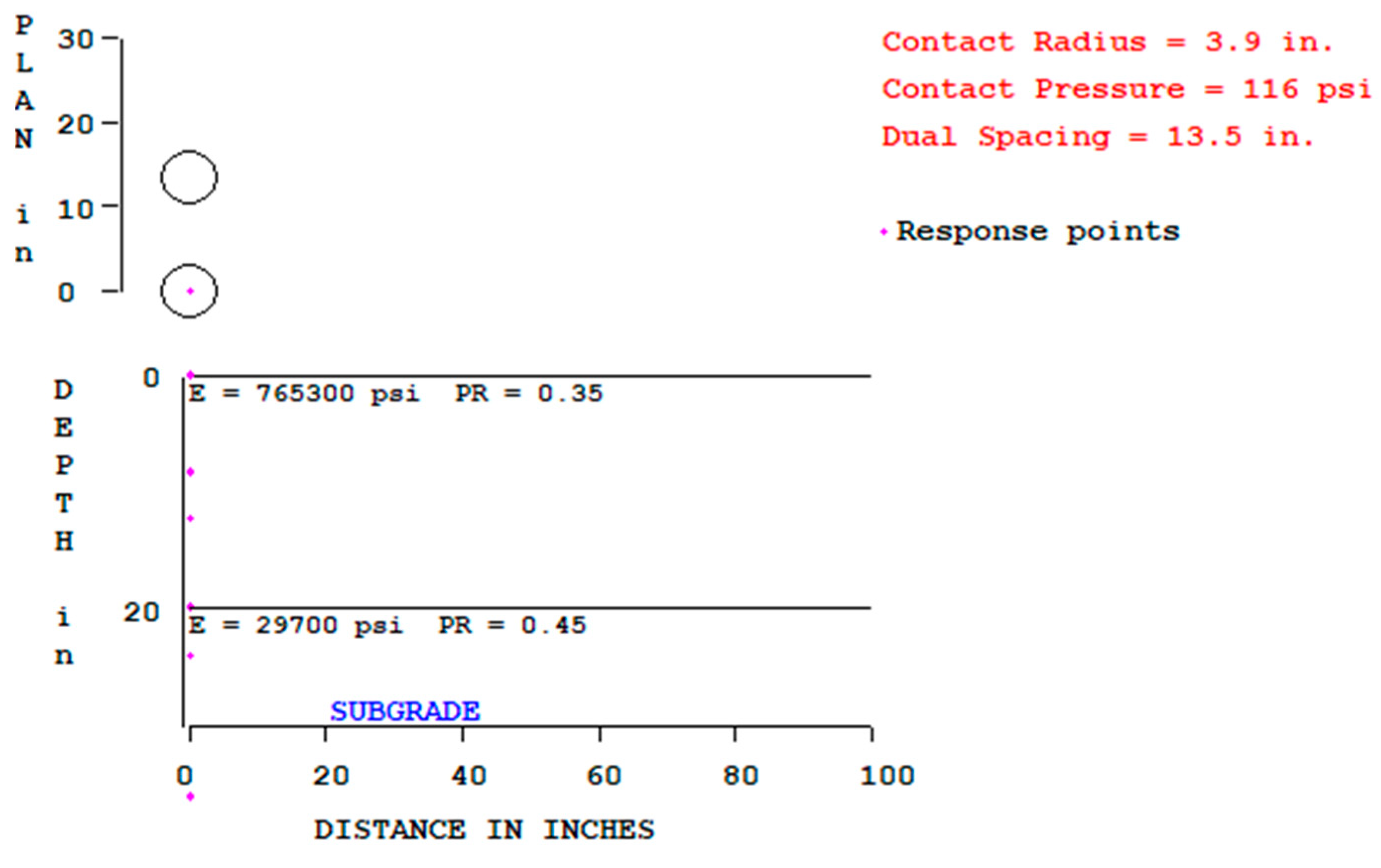
A Dynatest FFWD with seven geophone sensors (W1 to W7) was used for the FWD or FFWD test. The FWD tests were conducted at 359 locations or stations on the I-35 and SH-7 pavement sections. Modulus 7.0 [23] software was used to back-calculate elastic moduli for pavement layers and subgrade. For the purpose of this study, the strains at the bottom of the asphalt layer were determined using the KENLAYER software [18]. KENLAYER analyzes pavement using an elastic multi-layer system under a circular load applied on the pavement surface. During this analysis, load can be applied to layer systems using single, double, double tandem or double tridem wheels. In this study, two typical sections were adopted: one for I-35 that has 10 inches of asphalt concrete over 10 inches of Portland cement concrete and native subgrade, and the other being the pavement at the SH-7 section with 20 inches of asphalt concrete over native subgrade. The back-calculated elastic moduli from Modulus 7.0 were used in the KENLAYER analysis for each FWD location that matched with the TSD data. Figure 4 and Figure 5 show the typical layers for both sections. A contact radius of 3.9 in (99 mm.), contact tire pressure of 116 psi (800 kPa) and a dual spacing of 13.5 in. (342 mm.) were used as the load group. These values are standard for TSD loading. Also, deflection responses beneath the center of the wheel and tensile strain at the bottom of the AC layer were calculated. The following Poisson’s ratios were used in the analyzes by the KENLAYER software: 0.35 for AC, 0.15 for PCC and 0.45 for native subgrade. A total of 147 analyses for I-35 and 110 analyses for SH-7 were conducted using the KENLAYER software. Parameters such as wheel contact radius and pressure, wheel spacing, asphalt elastic moduli for asphalt, concrete and subgrade, and Poisson’s ratios were used as input parameters for each specific analysis.

Figure 4.
Typical section of I-35 used in KENLAYER analysis.
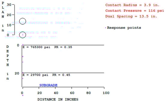
Figure 5.
Typical section of SH-7 used in KENLAYER analysis.
2.2. Approach of Strains and Effective Structural Number Calibration
In this study, deflection-basin-related indices or deflection bowl parameters were used to analyze deflection data from FWD and TSD and calibrate the model parameters. Deflection bowl parameters tend to focus mainly on the deflection under the center of the load (maximum deflection) and differences in deflection among the sensors as an indicator of the stiffness of different layers within the pavement structure, including the stiffness of the subgrade and the remaining life. The most common basin indices are Surface Curvature Index (SCI) (Equation (1)) and Deflection Slope Index (DSI) (Equation (2)). These indices are closely related to the condition of the upper layers of pavements. The SCI with r = 12 in. (300 mm.) is commonly used for deflection bowl analysis. Typically, s = 4 in. (100 mm.) and r = 12 in. (300 mm.) are used to calculate the DSI. Several other basin indices have been proposed by several researchers [24]. Their applications differ based on the layer that is intended to be analyzed. The area under the pavement (AUPP) is a deflection basin parameter that has been utilized successfully to link to horizontal strain at the base of the AC layer as well as to assess pavement stiffness (a lower AUPP equates to higher stiffness and vice versa) [25].
where
Ds and Dr represent deflections ‘’s’’, and ‘’r’’ inches away from the center of the load.
Rada et al. [13] proposed several TSD basin indices and models to calculate tensile strains at the bottom of the AC layer. The most prominent basin index was DSI4-12. Equation (4) describes the maximum fatigue strain as a function of DSI4-12. Coefficients or parameters “a” and “b” from Equation (4) were calibrated by comparing strains from KENLAYER analysis and DSI4-12 from TSD deflections. A non-linear regression analysis was used to calibrate model coefficients. Coefficients “a” and “b” were calibrated with a 90% confidence level along with outliers’ detection and removal techniques. Table 1 shows the most significant models based on AC layer thickness.

Table 1.
TSD index DSI4-12 and maximum fatigue or tensile strain [13].
The design of a pavement using the AASHTO method uses a structural indicator of pavements, known as “Structural Number (SN)” (previously called “thickness index”). It is used to determine the structural capacity or traffic load carrying capacity of a given pavement structure. In this method, contributions of all layers within the pavement structure are added to obtain the overall capacity of the pavement [24]. The SN determines the total number of ESAL a given pavement can support during its service life. Equation (5) describes the SN based on the layer coefficients, drainage coefficients, and layer thicknesses.
where
ai = ith layer coefficient;
Di = ith layer thickness;
mi = ith layer drainage coefficient.
The coefficients for asphalt concrete layer a1 can be determined by Equation (6) and Figure 6, as provided in the 1993 AASHTO Guide [2].
where
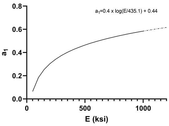
Figure 6.
Relationship of layer coefficient a1 and elastic moduli of AC [2].
a1 = 1st layer coefficient (AC).
Rhode [20] proposed Equation (7) to calculate the SNeff from the FWD measurements. For an asphalt pavement, Rhode proposed 0.4728, −0.4810, and 0.7581 as k1, k2, and k3, respectively. The k1, k2, and k3 values for determining SNeff with the TSD data were proposed by Nasimifar et al. [21] as 0.4369, −0.4768, and 0.8182, respectively.
where
HP = total thickness (mm);
SIP = structural index of pavement = D0 − D1.5HP.
In the present study, the model parameters proposed by Rhode [20] were calibrated by comparing the TSD data with the KENLAYER outputs. To calibrate Rhode’s [20] model parameters (k1, k2, and k3), two approaches were used in this study. The first approach involved using a non-linear regression calibration using FWD SNeff (Rhode’s method) and measured TSD deflections. The second approach used a non-linear regression calibration based on the calculated AASHTO SNeff and measured TSD deflections. In this approach, back-calculated moduli from the FWD were used to determine the asphalt layer coefficients using the AASHTO 1993 design charts. Layer coefficient a1 was calculated for each E modulus obtained from the I-35 and SH-7 sections based on the AASHTO 1993 design chart. A layer coefficient “a2” of 0.5 was assumed for the CRCP and JCP layers present in the I-35 section. Equation (5) was used to calculate SNeff with an assumed drainage coefficient of 1 for the CRCP and JCP layers. A non-linear regression analysis was used to calibrate parameters k1, k2, and k3, in Equation (7) for composite pavement sections on I-35. Coefficients k1, k2, and k3 were calibrated with a 90% confidence level along with outliers’ detection and removal techniques.
Also, an attempt was made to compare the elastic moduli obtained from the FWD and TSD data. Modulus 7.0 was used to back-calculate surface and subgrade elastic moduli from the FWD deflections. A similar approach was used to back-calculate surface and subgrade elastic moduli from the TSD deflections as well. For this purpose, the TSD data were formatted to Modulus 7.0 standards.
3. Results and Discussion
3.1. Traffic Speed Deflectometer Data
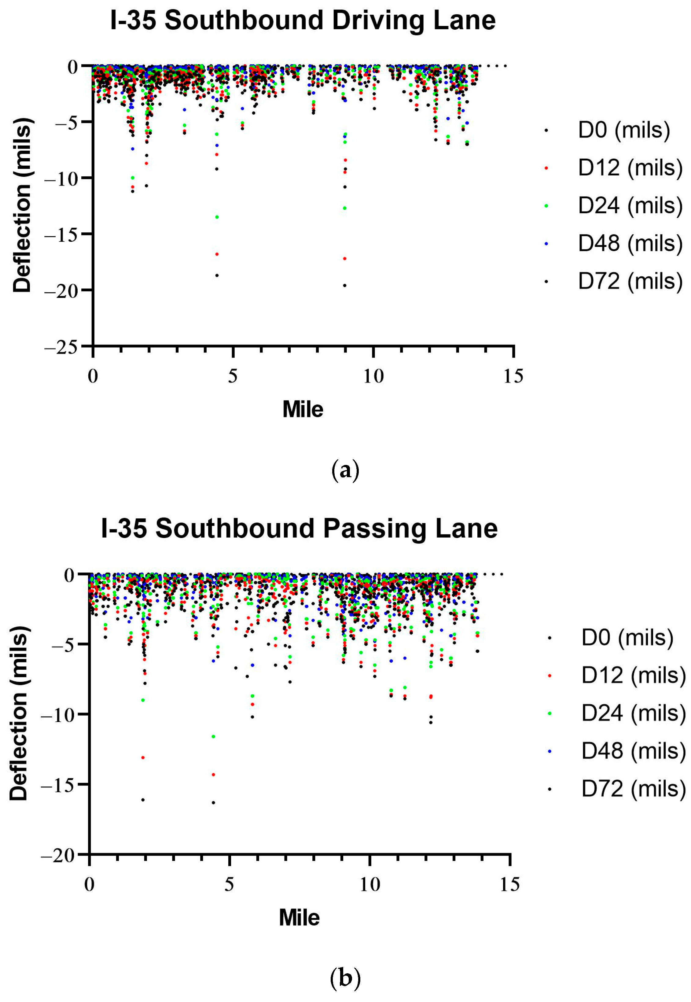
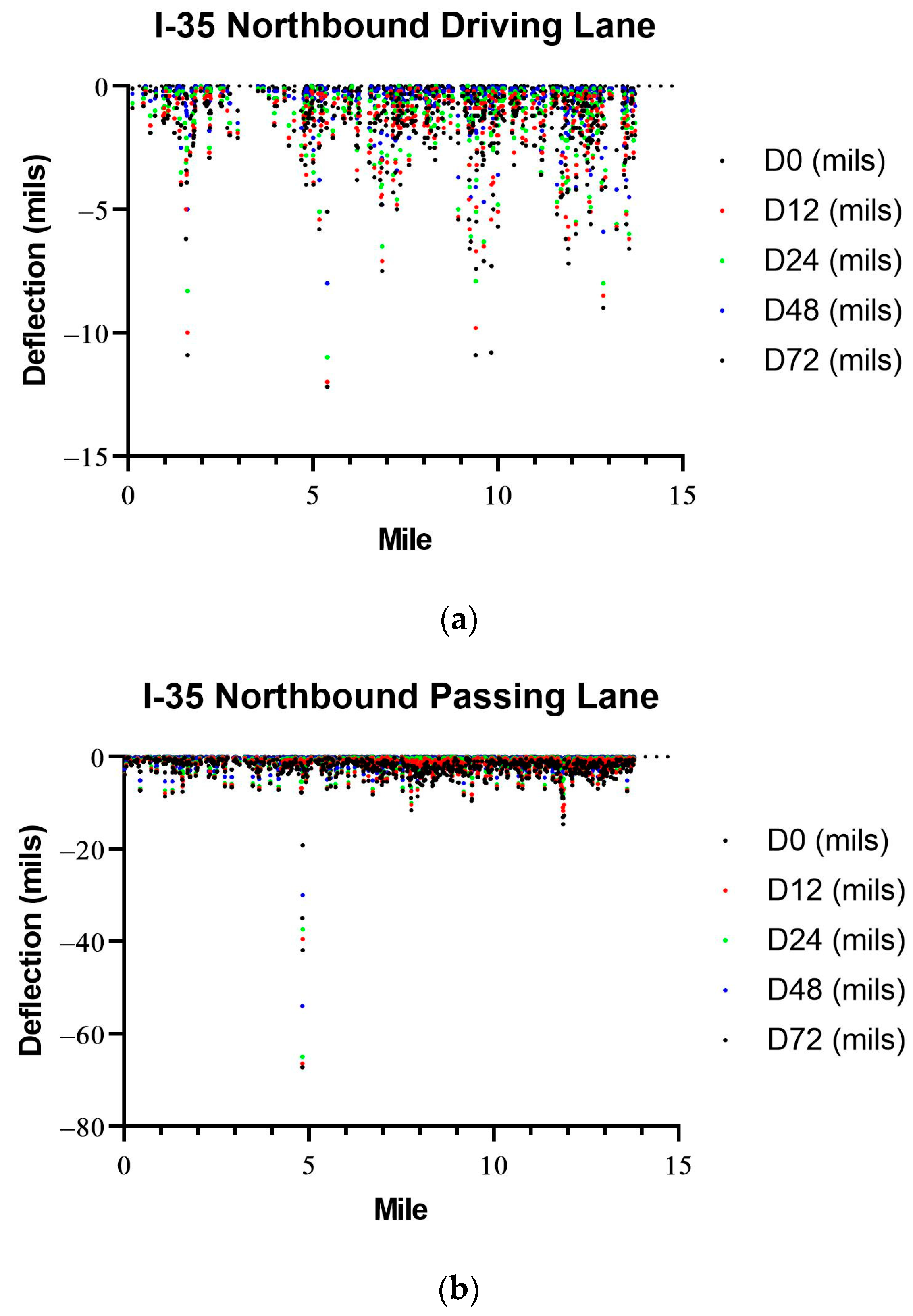
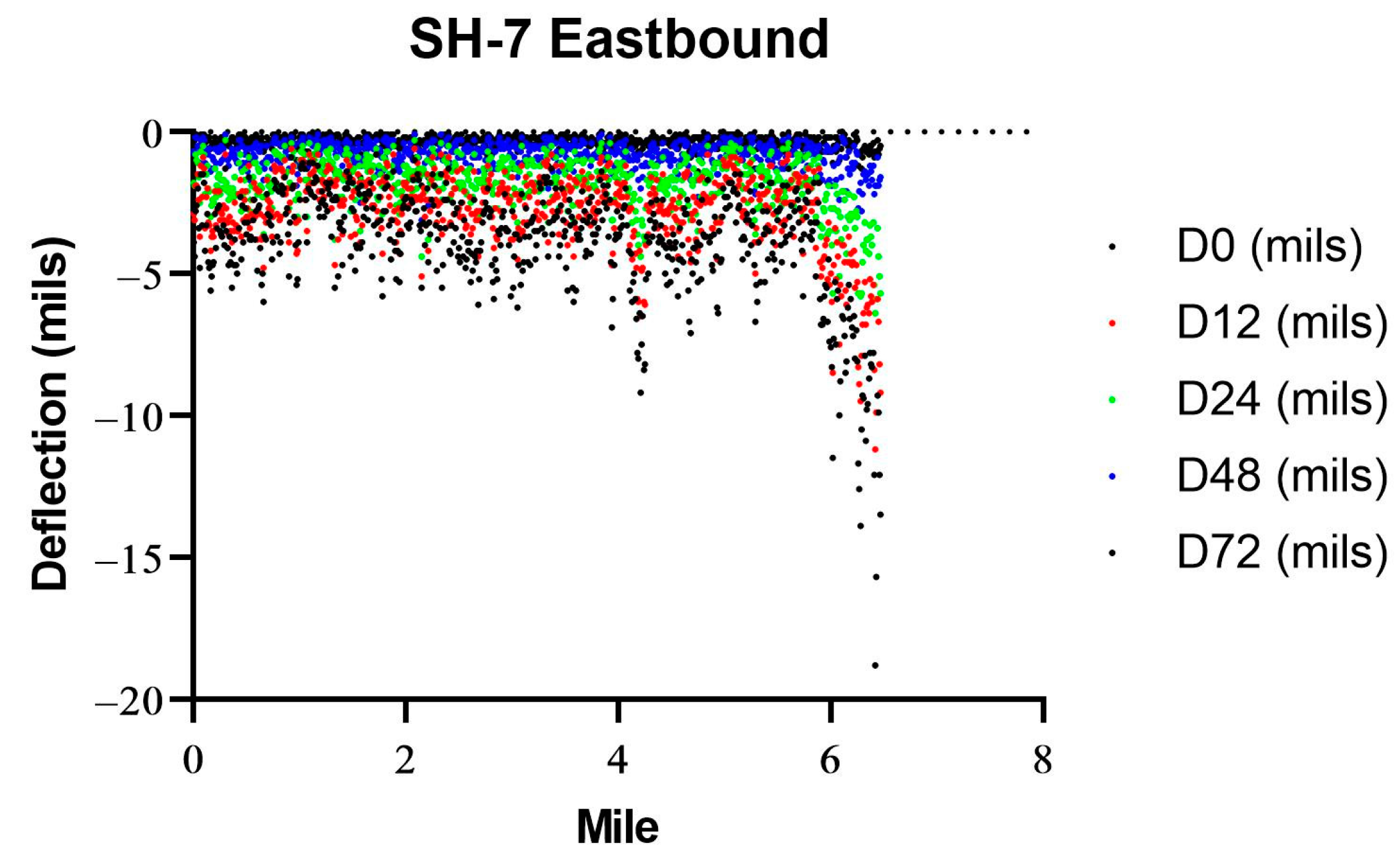
As mentioned above, FWD and TSD deflections, roughness and rut data were collected on I-35 and SH-7 sections. Figure 7, Figure 8, Figure 9 and Figure 10 show the deflection readings for the I-35 and SH-7 sections. For northbound I-35, mile 0 represents the starting point (Mile Post 45). For southbound I-35, mile 0 represents the ending point (Mile Post 59.5). For westbound SH-7, mile 0 represents the starting point (1 mile west of I-35). For eastbound SH-7, mile 0 represents the ending point (6 miles west of I-35). Generally, the passing lane had higher deflections compared to the driving lane of I-35 for both southbound and northbound lanes. For the SH-7 section, higher deflections were observed for both directions close to the starting point (1 mile west of I-35). A total of 535 and 543 points were analyzed for southbound driving lane and passing lane of I-35, with a mean maximum deflection (D0) of 1.9 and 2.2 mils, respectively. A total of 509 and 882 points were analyzed for the northbound driving lane and passing lane of I-35, with a mean maximum deflection (D0) of 1.9 and 2.6 mils, respectively. A total of 641 and 647 points were analyzed for the westbound and eastbound lanes of SH-7, respectively (Figure 8 and Figure 9). The mean maximum deflections (D0) of 3.6 and 3.9 mils were observed for the westbound and eastbound lanes of SH-7, respectively. As shown in Figure 7, Figure 8 and Figure 9, higher deflections were observed in passing lanes on I-35, where no reflection cracking due to JCP and CRCP pavements was observed.
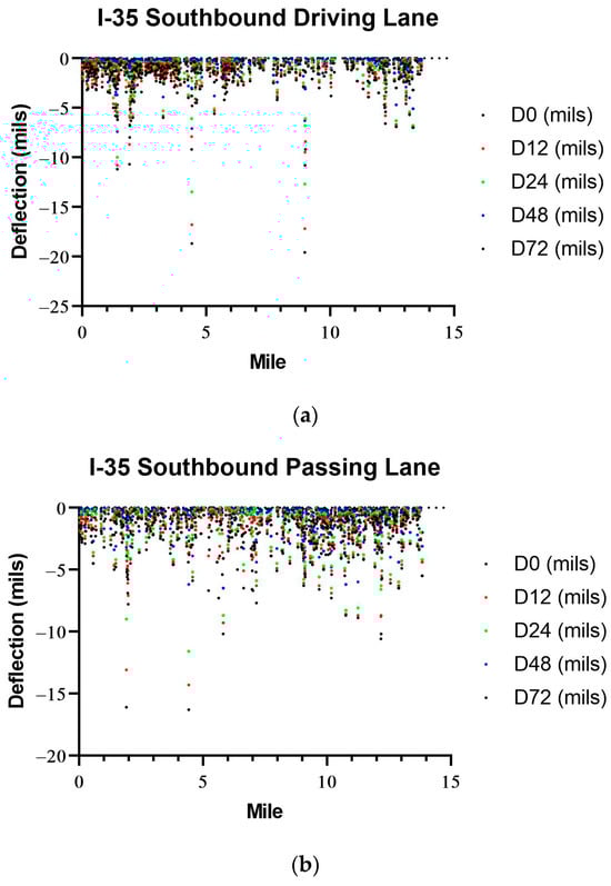
Figure 7.
TSD deflections on the (a) driving and (b) passing lanes of Southbound I-35.
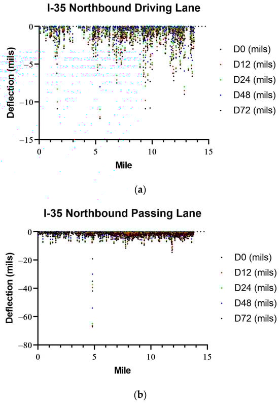
Figure 8.
TSD deflections on the (a) driving and (b) passing lanes of Northbound I-35.
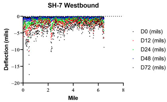
Figure 9.
TSD deflections on Westbound SH-7.

Figure 10.
TSD deflections on Eastbound SH-7.
3.2. Falling Weight Deflectometer Data
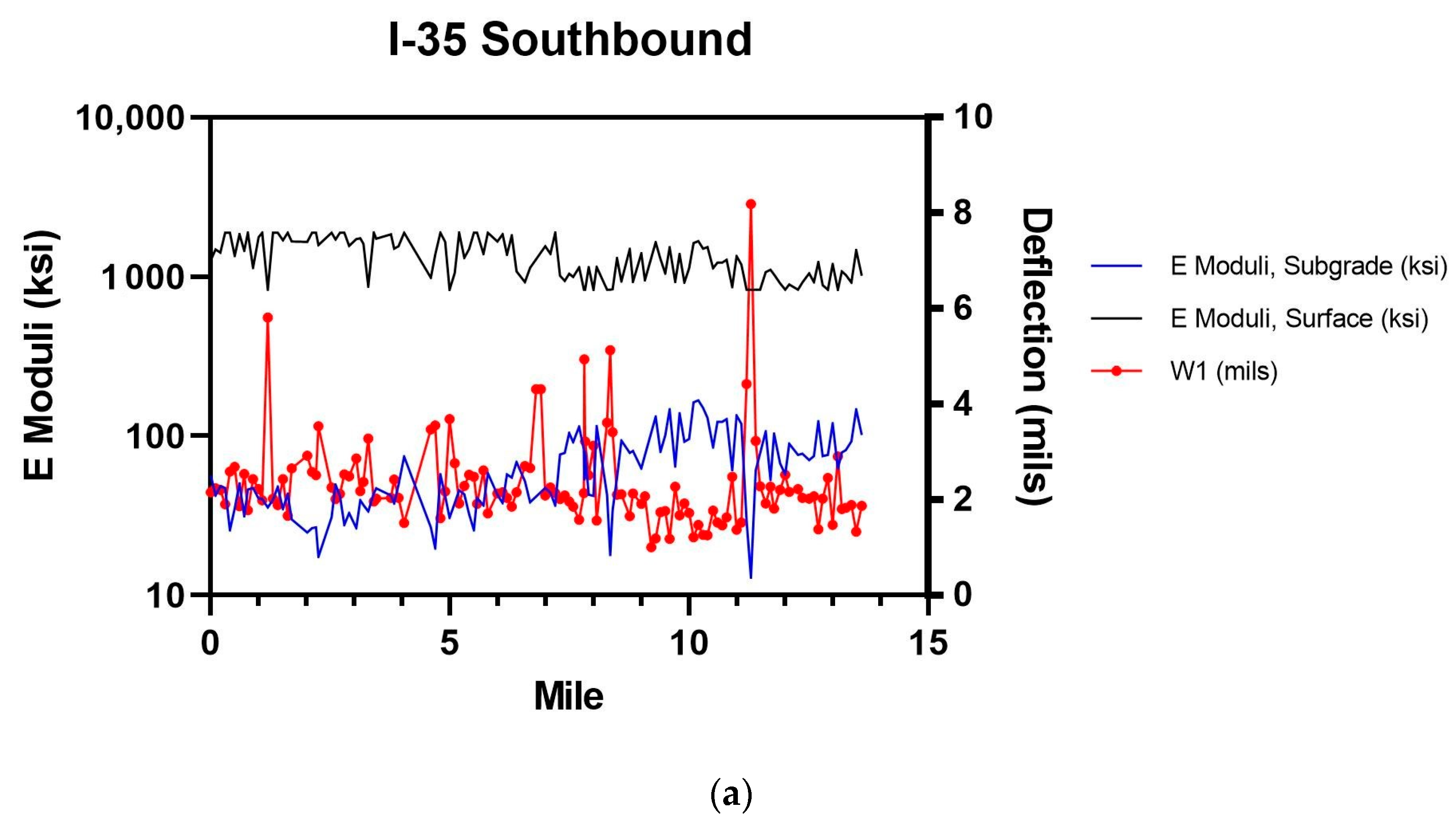
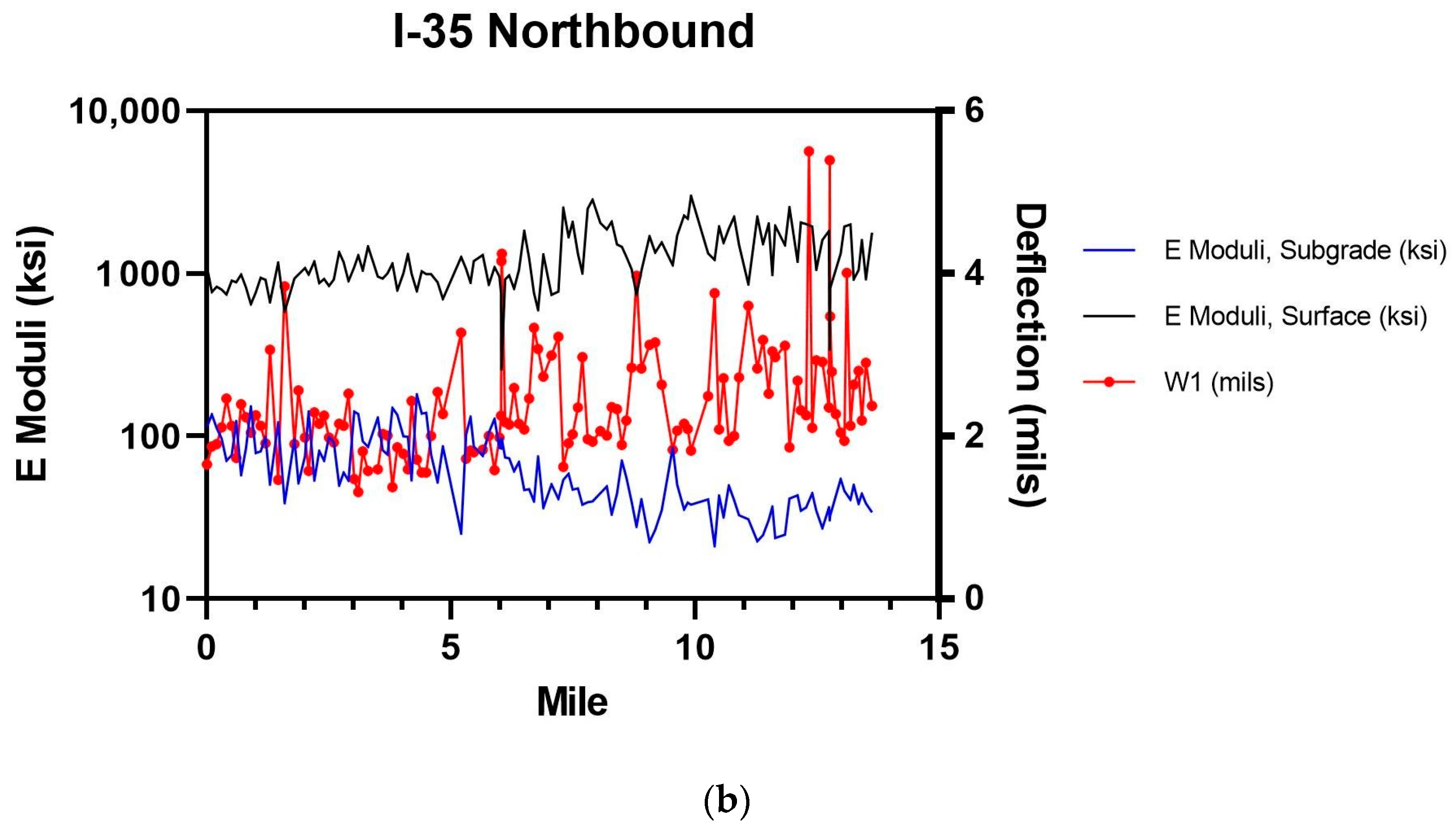
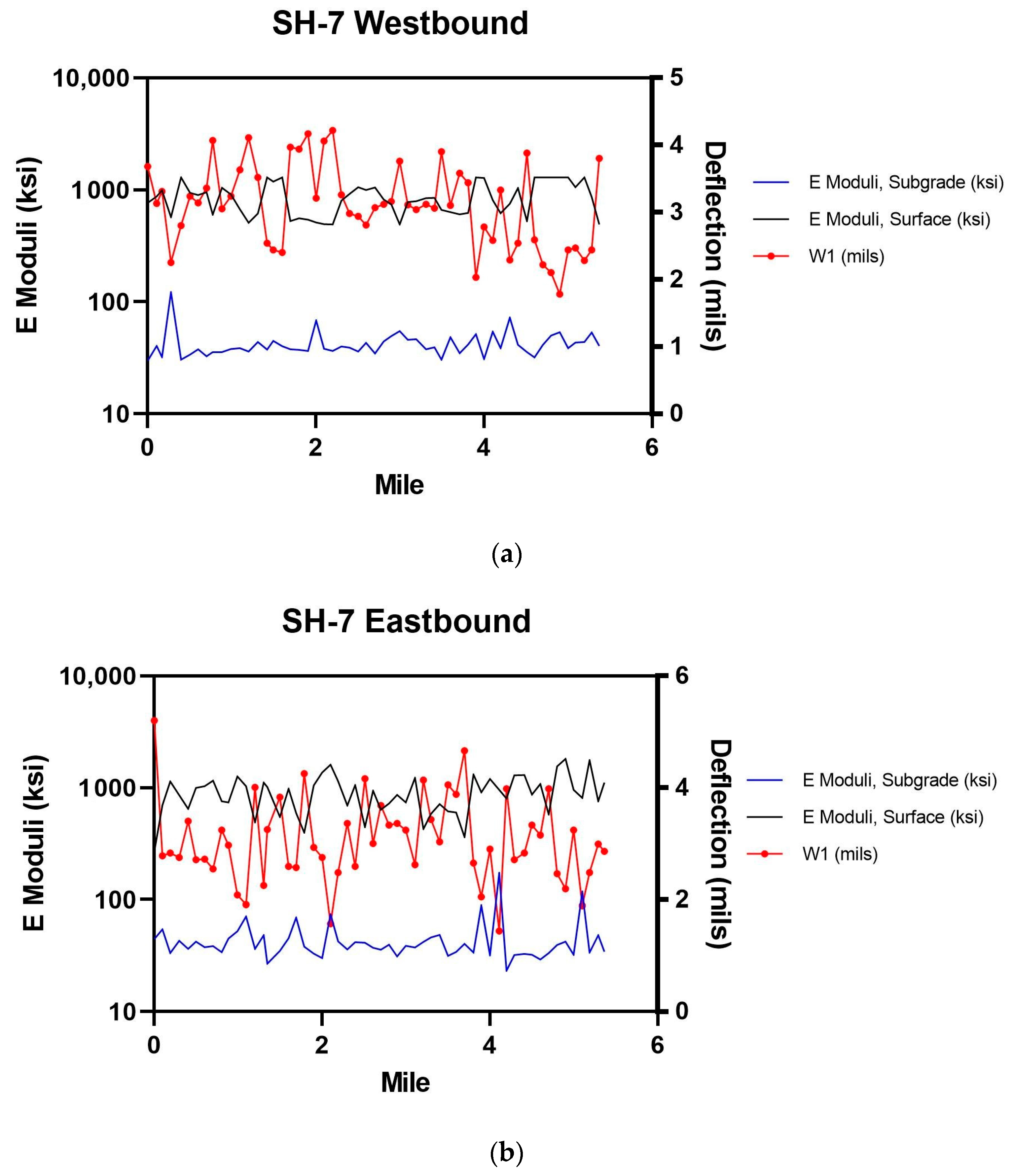
Falling Weight Deflectometer or FFWD data were collected on the I-35 and SH-7 sections. Modulus 7.0 was used to back-calculate elastic moduli for the pavement layers and subgrade. The deflection and elastic moduli values for the northbound and southbound sections of I-35 are shown in Figure 11, while the deflection and elastic moduli values for the eastbound and westbound sections of SH-7 are shown in Figure 12. For safety reasons, FWD tests were performed only on the right-most lane (next to the shoulder) in each direction (i.e., the driving lane). The deflection values at the center of the FWD loading plate correspond to the W1 sensor, which is an indicator of the overall structural condition of the pavement at the time of testing. The W7 sensor, on the other hand, indicates deflection at 60 inches (1500 mm) from the center of the load, which is an indicator of the subgrade strength. The air temperature during testing ranged from 32 °F to 51 °F (0 to 11 °C), as per temperature data collected from the Mesonet site located at Pauls Valley, Oklahoma. For the northbound lane of I-35, FWD tests were conducted at 124 locations. Comparatively, FWD tests at the southbound lane of I-35 were conducted at 123 locations. For the eastbound and westbound lanes of SH-7, FWD tests were conducted at 56 locations in each direction. These measurements and calculations were used in this study to obtain tensile strains at the bottom of the asphalt layer, to compare with the TSD data, and to calibrate the model parameters.
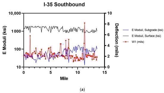
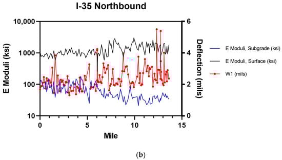
Figure 11.
FWD elastic moduli and deflections for (a) southbound and (b) northbound lanes of I-35.
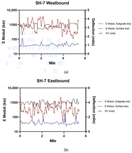
Figure 12.
FWD elastic moduli and deflections for (a) westbound and (b) eastbound lanes of SH-7.
3.3. KENLAYER Analysis and Comparison with TSD and FWD Data
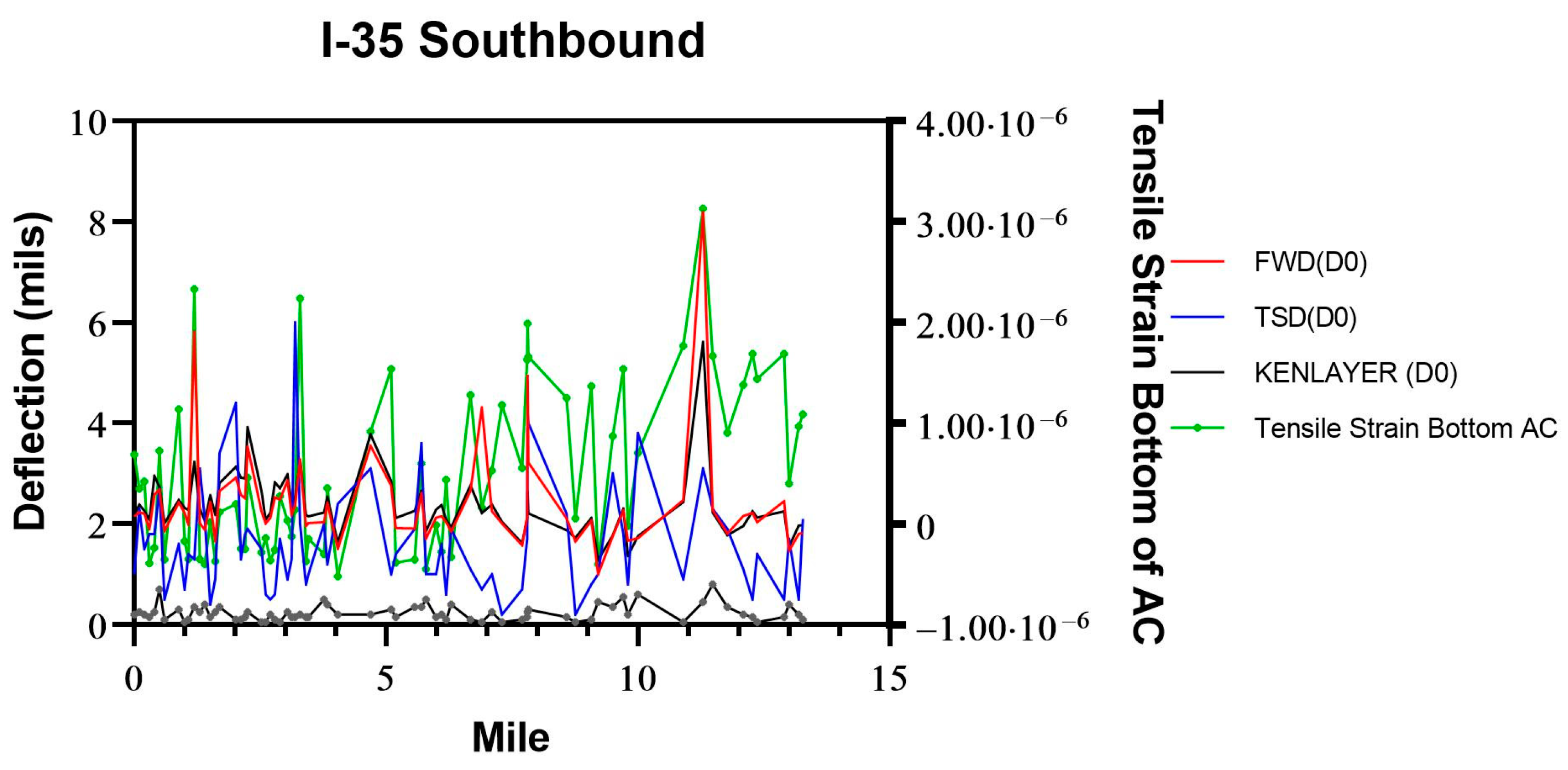
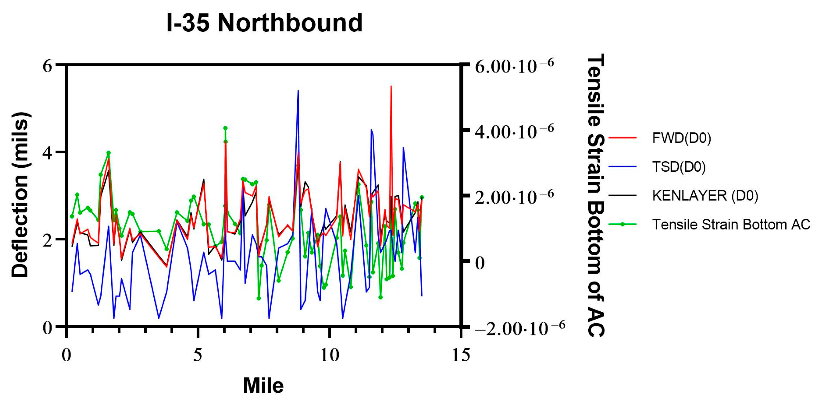
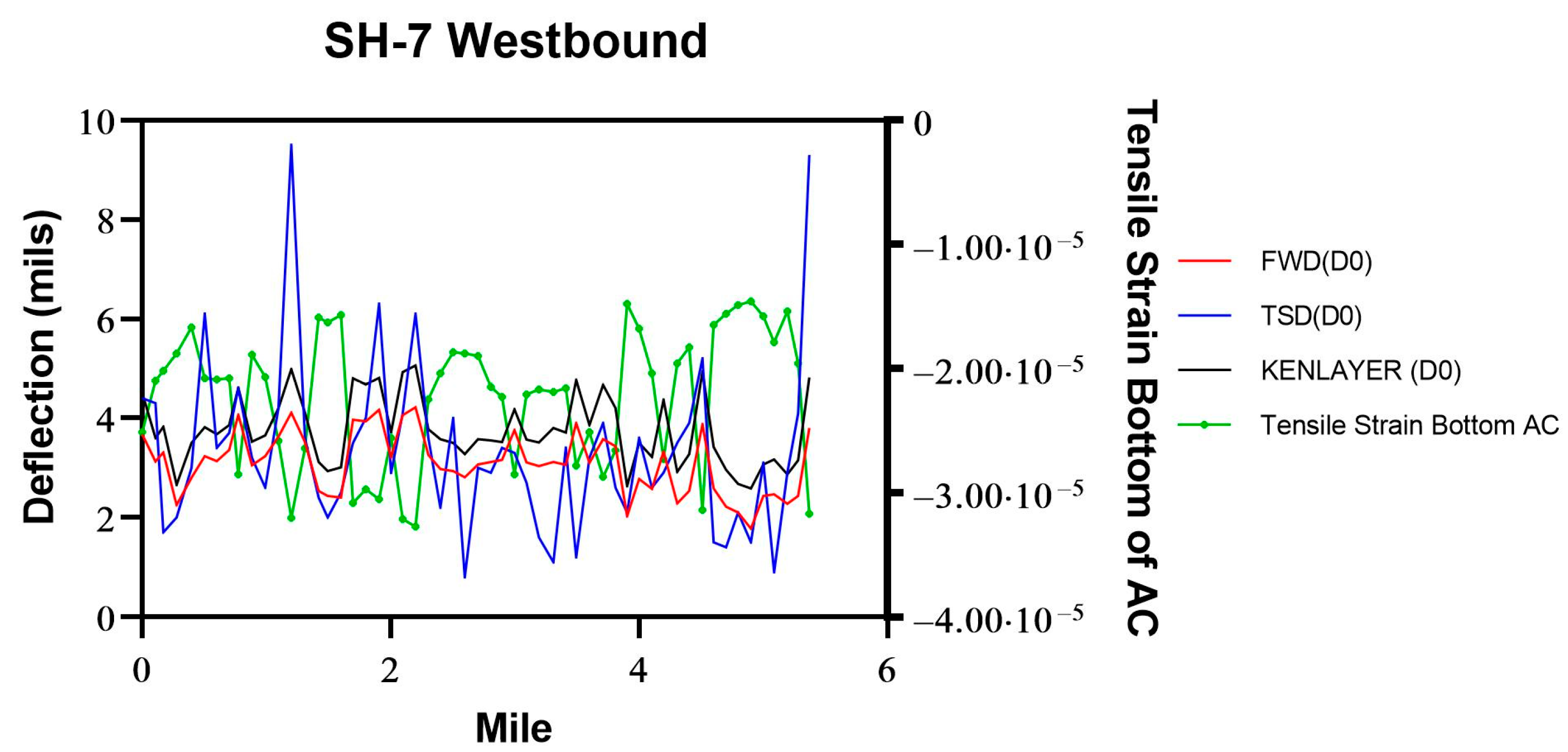
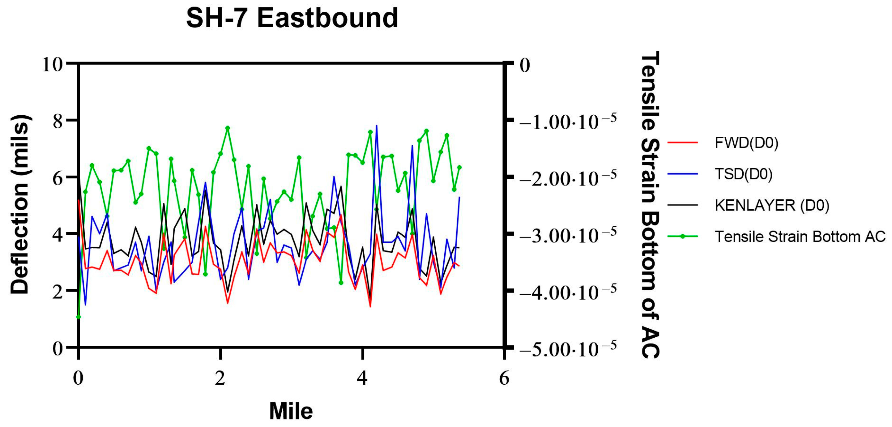
A total of 147 analyses for I-35 and 110 analyses for SH-7 were carried out using the KENLAYER software. Each analysis was conducted using a different set of elastic moduli. Figure 13, Figure 14, Figure 15 and Figure 16 show the tensile strains at the bottom of AC layer and the deflections at the top of the AC layer from the KENLAYER analyses, along with FWD and TSD maximum deflections (D0) for comparison purposes. It can be observed that the KENLAYER and FWD deflections were similar in all directions for both the I-35 and SH-7 sections. This was expected as the elastic moduli input for KENLAYER analyses was based on the FWD data. Better relations were observed between TSD, FWD and KENLAYER deflections for the SH-7 section compared to the I-35 section.
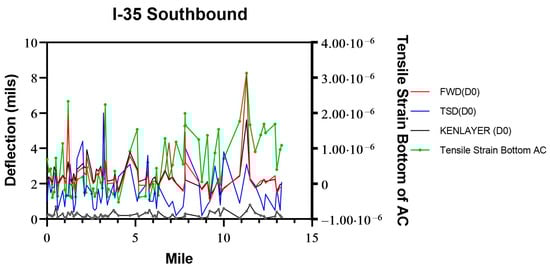
Figure 13.
Comparison of deflections and strains obtained from different methods for the southbound lanes of I-35.
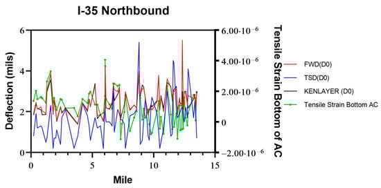
Figure 14.
Comparison of deflections and strains obtained from different methods for the northbound lanes of I-35.
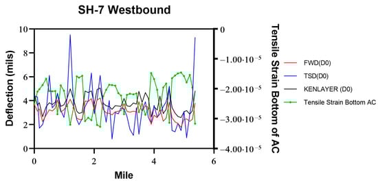
Figure 15.
Comparison of deflections and strains obtained from different methods for the westbound lanes of SH-7.
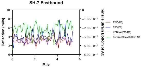
Figure 16.
Comparison of deflections and strains obtained from different methods for the eastbound lanes of SH-7.
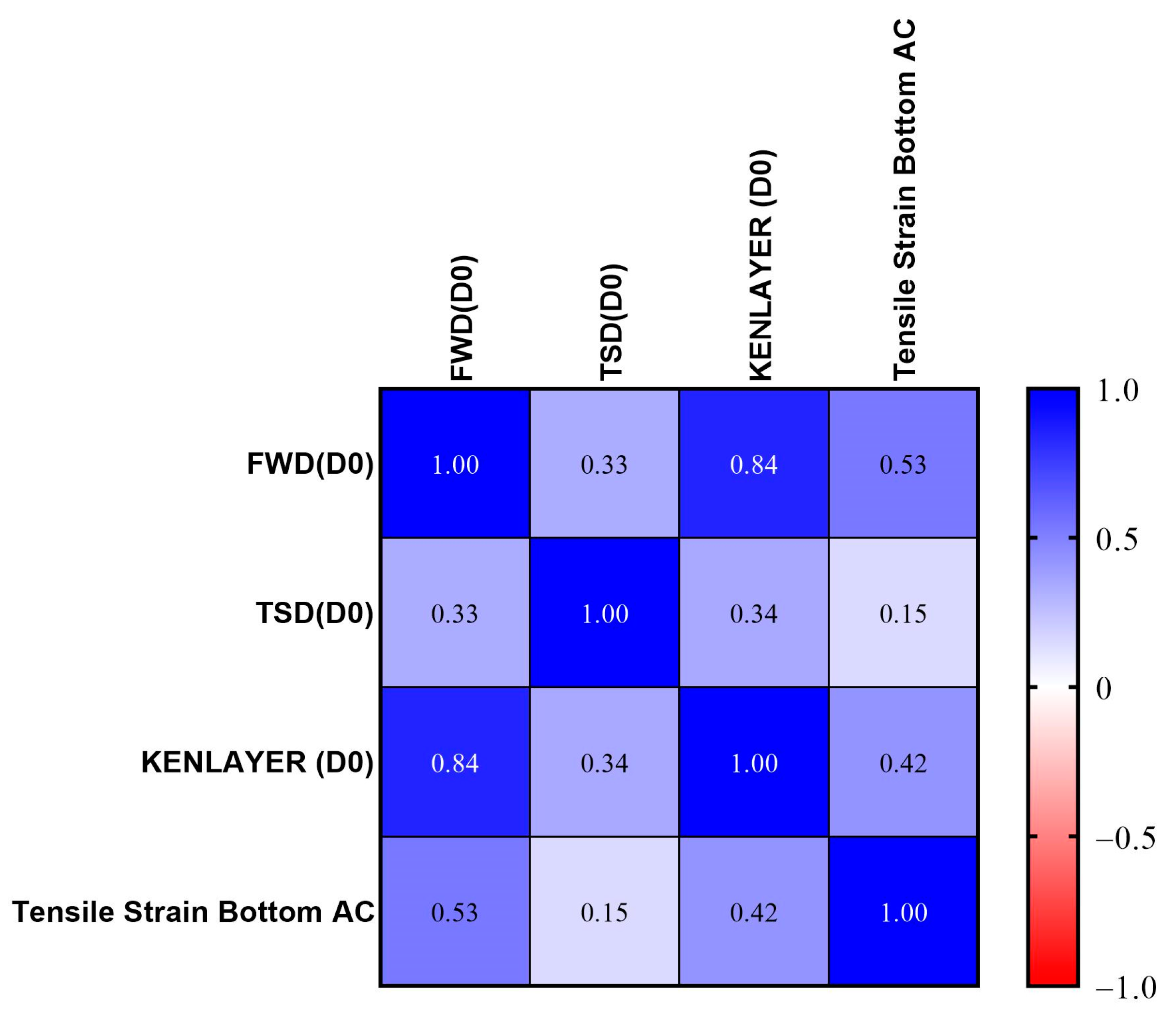
Figure 17 and Figure 18 show the Pearson (r) correlations between the tensile strain at the bottom of AC and TSD and FWD deflections for I-35 and SH-7 sections, respectively. From Figure 16, tensile strain at the bottom of the AC layer from the KENLAYER analyses was found to exhibit a better correlation with the FWD deflections.

Figure 17.
Pearson (r) correlation matrix for deflections and tensile strains for the I-35 section.
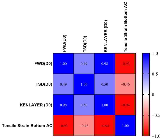
Figure 18.
Pearson (r) correlation matrix for deflections and tensile strains for the SH-7 section.
Figure 18 exhibited relatively higher correlations between deflections obtained from TSD, KENLAYER and FWD for the SH-7 section. Strong correlations were observed (with an r value > 0.53 for the I-35 section and >0.84 for the SH-7 section) between the tensile strains at the bottom of the AC layer obtained from the KENLAYER analyses and FWD deflections. Also, for the SH-7 section, tensile strains at the bottom of the AC layer showed better correlations with the TSD compared to that of the I-35 section. For the I-35 section, an overall compressive strain at the bottom of the AC layer was observed (Figure 13 and Figure 14). This was due to the composite nature of the I-35 section, which produced a neutral axis below the asphalt layer and resulted in compressive strain at the bottom of the asphalt layer. Tensile strains were observed at the bottom of the asphalt layer for the SH-7 section due to the direct contact with a softer layer or native subgrade.
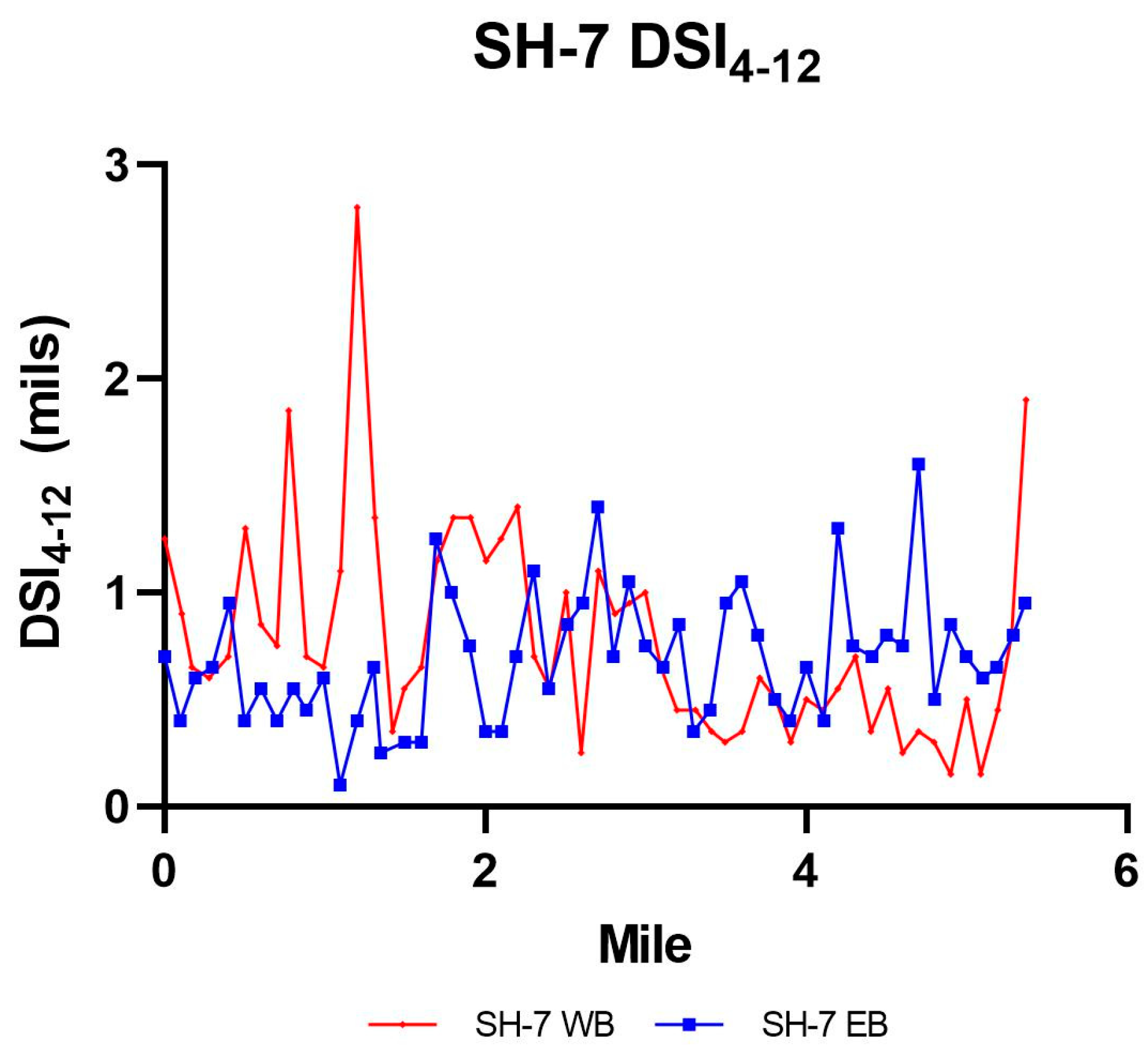
Figure 19 and Figure 20 show the DSI4-12 values obtained from the TSD data for the I-35 and SH-7 sections, respectively. The depths of the AC layers were 10 inches for the I-35 section and 20 inches for the SH-7 section. Equation (4) describes the maximum fatigue strain as a function of DSI4-12.
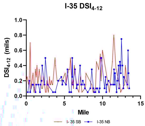
Figure 19.
Deflection Slope Index (DSI) obtained from the TSD data for the I-35 section.

Figure 20.
Deflection Slope Index (DSI) obtained from the TSD data for the SH-7 section.
3.4. Calibration of Tensile Strain Model Coefficients
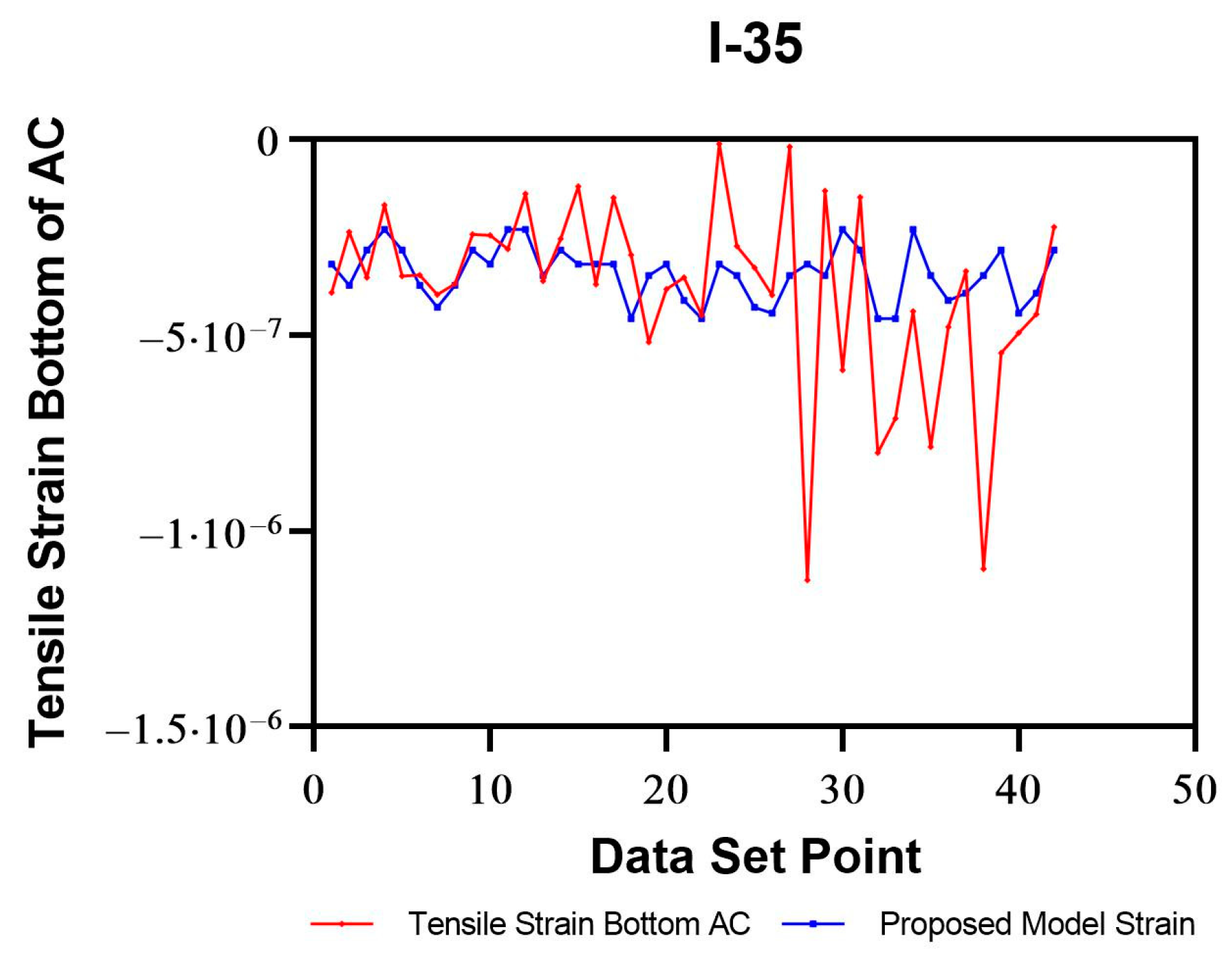
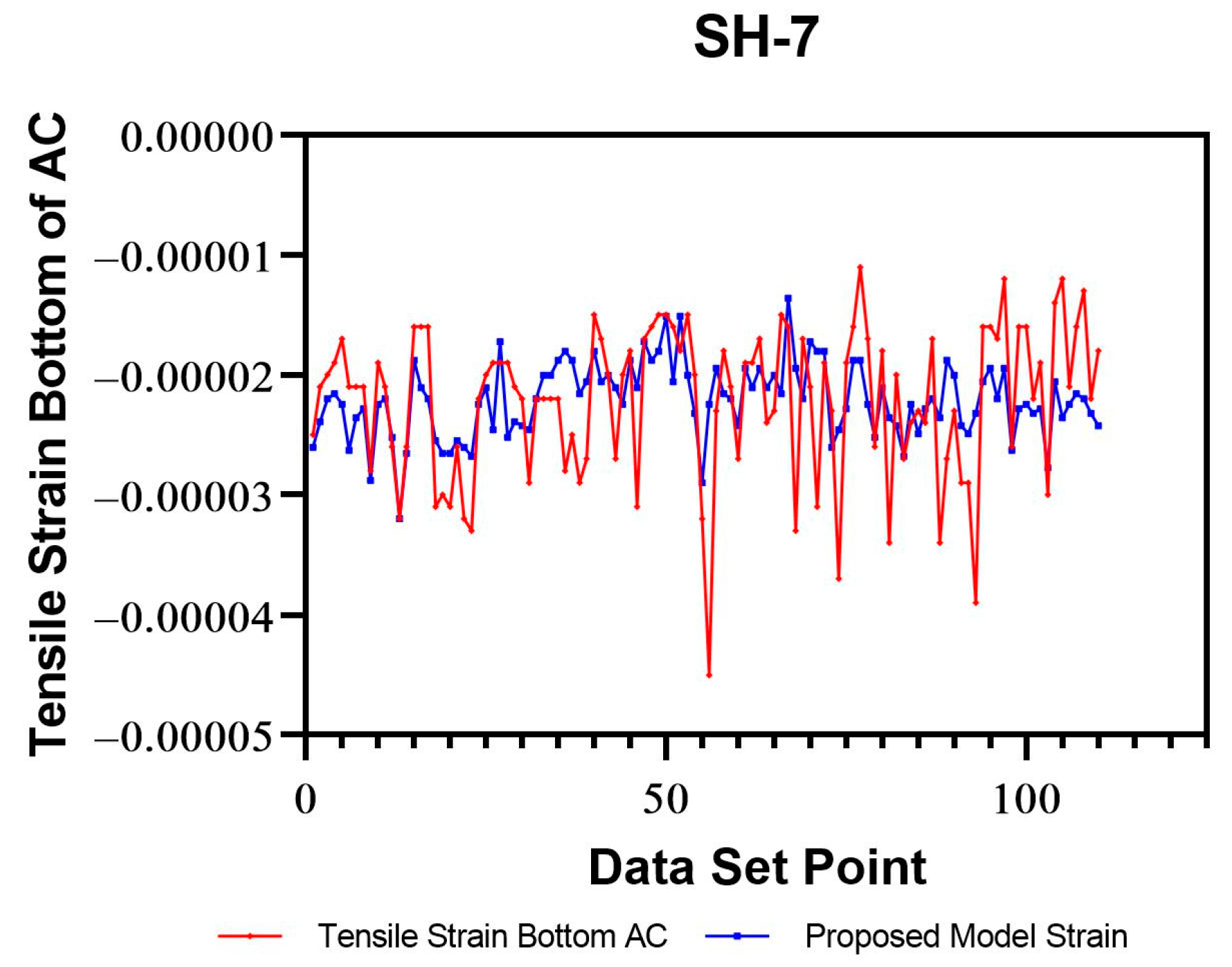
As noted earlier, when calculating tensile strains at the bottom of the AC layer using the KENLAYER software, several data points on I-35 showed compressive strain instead of tensile strain. This change in behavior generally occurred when the AC elastic moduli values were below 1700 ksi, as can be observed in Figure 21. This is due to the composite nature of the I-35 section mentioned above. This was not observed for the SH-7 section, where a softer native subgrade (assumed to be semi-infinite) layer was present underneath the AC layer. Only 42 data points showed tensile strains at the bottom of the AC layer on the I-35 section. These 42 data points were used to fit the non-linear Equation (4) proposed by Rada et al. [13] and to calculate the corresponding parameters “a” and “b”. The coefficient “a” ranged from −0.9054 to −0.3310 and the coefficient “b” ranged from −0.06168 to 0.5535, with the best fit values being −0.5645 and 0.2297 for coefficients “a” and “b,” respectively. Figure 22 shows a comparison between the strain at the bottom of the AC from KENLAYER and the strains calculated from Rada et al.’s [13] calibrated model. As mentioned above, for the SH-7 section, the strains at the bottom of the AC layer were in tension. The corresponding coefficient “a” ranged from −25.9 to −23.22 and coefficient “b” ranged from 0.1657 to 0.3486, with the best fit values being −0.2457 and 0.2566 for coefficients “a” and “b”, respectively. Figure 23 shows a comparison between the tensile strains and the model-calculated strains. An r correlation of 0.5 was observed.
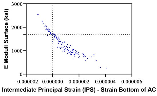
Figure 21.
Tensile strains and surface E moduli for the I-35 section.
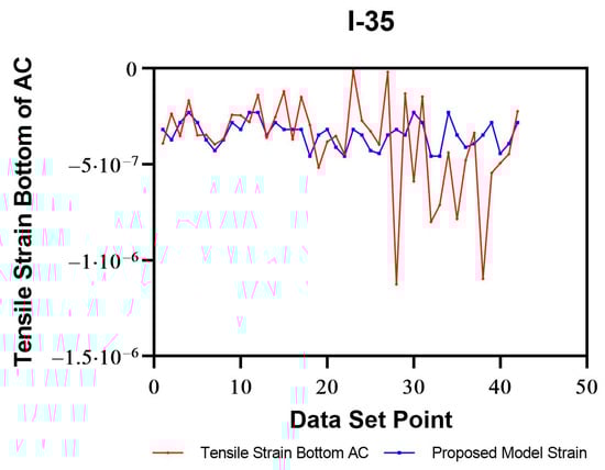
Figure 22.
Comparison of tensile strains from KENLAYER and Rada et al.’s [13] calibrated model for the I-35 section.
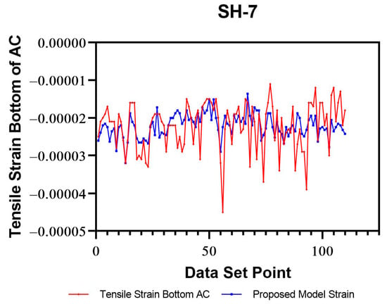
Figure 23.
Comparison of tensile strains from KENLAYER and calibrated Rada et al. [13] model for the SH-7 section.
3.5. Calibration of Effective Structural Number Model Coefficients
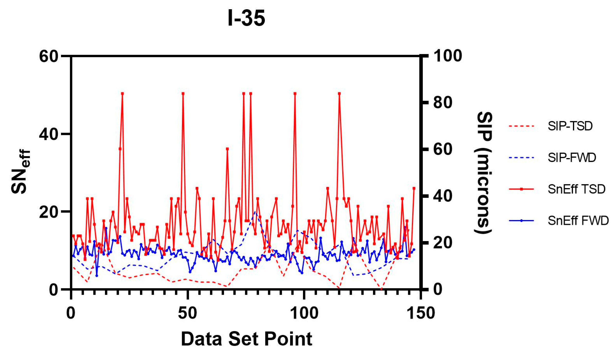
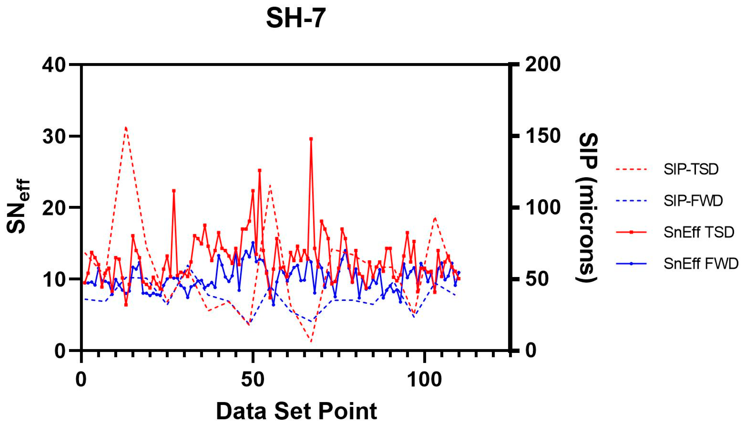
In this study, an attempt was made to calibrate the parameters of Equation (7) for an accurate determination of SNeff from TSD measurements. As shown in Equation (7), the model uses a structural index of pavement (SIP) to calculate the SNeff from the deflection measurements. Figure 24 and Figure 25 show the correlations between SNeff and SIP based on the FWD and TSD and the Rhode [20] and Nasimifar et al. [21] models for the I-35 and SH-7 sections. A poor correlation (r < 0.1) was observed for SNeff from FWD and TSD data for I-35, as shown in Figure 24. However, a better correlation was observed for the SIP from the FWD and TSD. A higher r correlation was observed for SH-7 data for the SIP and SNeff from the FWD and TSD. r values of 0.54 and 0.52 were observed for SNeff and SIP between the FWD and TSD data sets for SH-7.
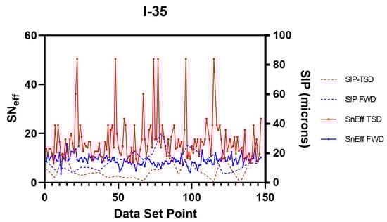
Figure 24.
Comparison of SNeff and SIP for the I-35 section.
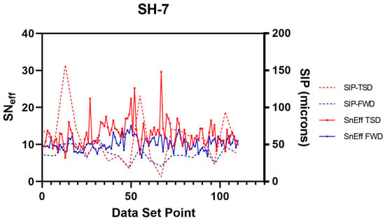
Figure 25.
Comparison of SNeff and SIP for the SH-7 section.
As noted earlier, to calibrate k1, k2, and k3 in Equation (7) for TSD measurements, two approaches were used in this study. The first approach involved using a non-linear regression calibration from FWD SNeff (Rhode’s method) and measured TSD deflections. The second approach used a non-linear regression calibration based on calculated AASHTO SNeff and measured TSD deflections. In this approach, back-calculated elastic moduli from the FWD were used to determine the asphalt layer coefficients using the AASHTO 1993 design charts. Figure 6 shows the a1 layer coefficient based on the asphalt concrete elastic moduli.
3.5.1. Calibration of Effective Structural Number Model Based on Rhode’s Method
A non-linear regression analysis was used to calibrate parameters k1, k2, and k3, in Equation (7). For this purpose, target SNeff values were calculated by the Rhode equation using the FWD data. The SIP and layer thicknesses from TSD were used to fit the model and to calculate the parameters. The parameters k1, k2, and k3 were modeled with a 90% confidence interval along with outliers’ detection and removal. For the I-35 section, the calibrated values for the parameters k1, k2, and k3 were found to be 0.2796, −0.01121, and 0.6296, respectively. Figure 26 shows the SNeff values calculated by Rhode’s equation using the FWD data and the SNeff values from TSD data using the calibrated model parameters for the I-35 sections. The overall correlation was observed to be low. For the SH-7 section, the calibrated values for the parameters k1, k2, and k3 were found to be 0.3131, −0.1797 and 0.6639, respectively. Figure 27 shows a comparison of the SNeff values calculated by Rhode’s equation using the FWD data and the predicted SNeff values from TSD data using calibrated model parameters for the SH-7 sections. An improved correlation with an R value of 0.55 was observed for the SH-7 section. As described in the previous sections, the application of Rada et al.’s [13] and Rhode’s [20] equations may be limited for composite pavements.

Figure 26.
Comparison of SNeff Values for the I-35 section predicted using the Rhode equation, FWD data, and calibrated model.
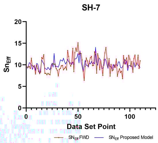
Figure 27.
Comparison of SNeff values for the SH-7 section predicted using the Rhode equation, FWD data, and calibrated model.
3.5.2. Calibration of Effective Structural Number Model Based on the AASHTO Method
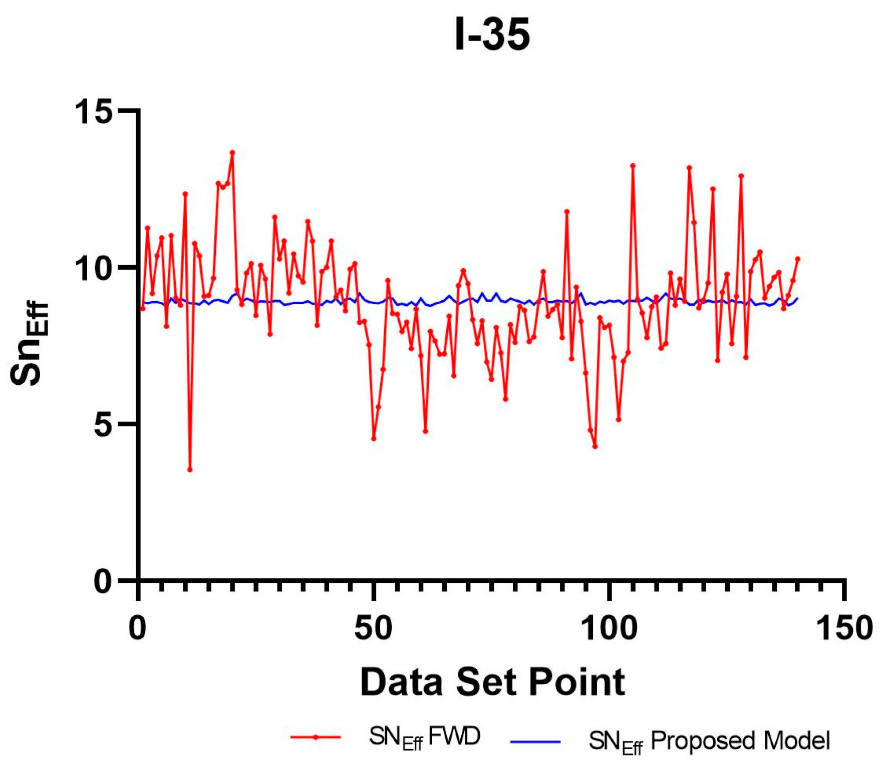
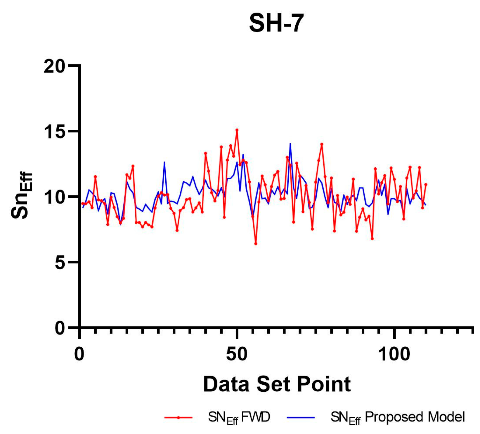
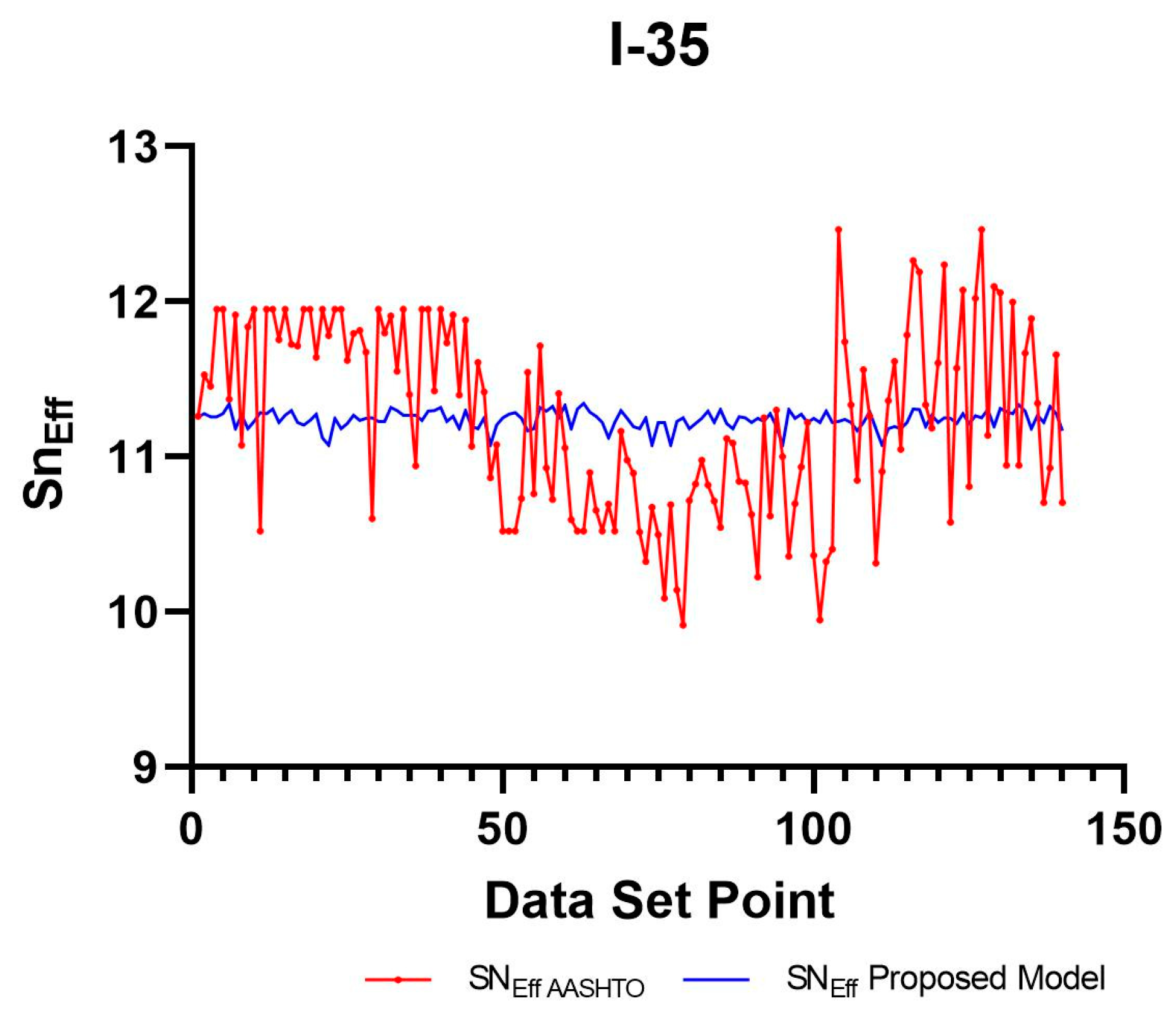
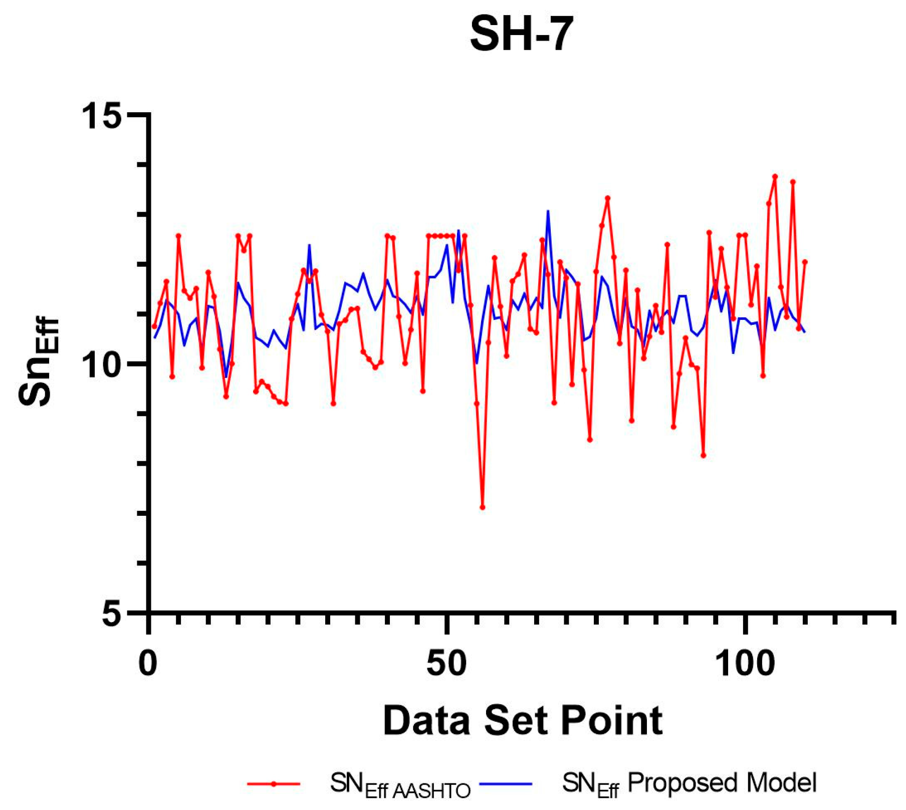
Layer coefficients a1 were calculated for each elastic moduli obtained from the I-35 and SH-7 sections based on the AASHTO 1993 design chart shown in Figure 6. A layer coefficient “a2” of 0.5 was assumed for the CRCP and JPCP layer present in the I-35 section. Equation (5) was used to calculate SNeff with an assumed drainage coefficient of 1 for the CRCP and JCPC layers. Coefficients k1, k2, and k3 were modeled with a 90% confidence interval along with the outliers’ detection and removal techniques. For the I-35 section, the parameters k1, k2 and k3 were found to be 0.3122, 0.00247, and 0.6457, respectively. Figure 28 shows the SNeff values calculated using the AASHTO method and the predicted SNeff values from the TSD data using calibrated model parameters for I-35 sections. An overall low correlation was observed. For the SH-7 section, the corresponding values for parameters k1, k2, and k3 were 0.2747, 0.09122, and 0.6470, respectively. Figure 29 shows the SNeff values calculated using the AASHTO method and the predicted SNeff values using the model parameters for SH-7. Overall, better results were observed for SH-7, with an r correlation higher than 0.4.
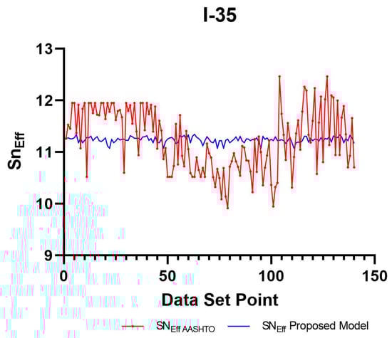
Figure 28.
Comparison of SNeff obtained from the AASHTO method and the TSD data using calibrated model for I-35.
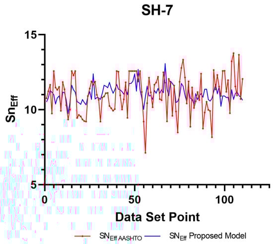
Figure 29.
Comparison of SNeff obtained from the AASHTO method and the TSD data using calibrated model for SH-7.
4. Conclusions
The main objective of the study was to review, compare, analyze, and model the TSD data from I-35 and SH-7 sections that were collected in the State of Oklahoma. Data from TSD were compared with FWD data. In this study, the KENLAYER software was used to model deflections, strains, and stresses for asphalt concrete pavements for the SH-7 section, and composite pavements for the I-35 section. Also, GPR data and coring were further analyzed to determine thicknesses. The models for calculating tensile strain at the bottom of the AC layer and SNeff were calibrated for TSD data. The overall findings of this study are listed below:
- The TSD data from the I-35 sections showed inconsistencies, with missing deflection values at various points. Factors such as the pavement’s properties (like its composite nature or stiffness), slight deflections, recording speed, or issues with the laser capturing velocities might have contributed. Due to this, some FWD deflections were left out of our comparison.
- The elastic modulus values for the surface and subgrade layers of the I-35 and SH-7 sections were determined using the FWD test data. Overall, good modulus (E) values were observed for the I-35 section but low modulus values were observed for the eastbound inside lane of the SH-7 section. The TSD data were organized in the format used by Modulus 7.0 and used to back-calculate elastic moduli. Attempts were made to correlate the FWD deflections with the TSD deflections. Deflections from TSD testing showed better correlations for the SH-7 section when compared with the FWD and KENLAYER deflections.
- Tensile strains identified at the base of the asphalt concrete layer via KENLAYER displayed varying patterns for composite pavements. Notably, tension was not observed across all studied sections at the base of AC in composite pavements. Often, a more rigid layer underneath the asphalt concrete led to compression, not tensile strains, at the asphalt layer’s base. In the I-35 section, this was particularly evident when the elastic moduli of the asphalt layers dropped below 1700 ksi. Conversely, for non-composite pavements, anticipated tensile strains were consistently noted at the asphalt concrete layer’s base. During this study, the parameters were for extracting tensile strains from TSD basin metrics (DSI). Notably, a stronger correlation was seen between the newly calibrated coefficients and the standard TSD ones for the SH-7 section.
- Parameters or coefficients for effective structural number from TSD data were calibrated using FWD data. The Rhode method correlated better than the AASHTO method. Also, better correlations were observed for the SH-7 section, in general.
- The study conducted a comprehensive analysis of pavement behavior using TSD and FWD data. Different sections and directions were studied, revealing insights into deflections, strains, and correlations. The study also highlighted the importance of calibration for accurately determining structural parameters from measurements. The findings have implications for understanding pavement performance and designing road infrastructure more effectively.
The TSD is gaining popularity in pavement management at the network level. From the results presented in this paper, it is evident that its application at the project level is promising. The structural capacity of roads can be assessed at a much faster rate and with wider coverage. This can help the decision making of PMSs for MRR’s applications. Hence, the remaining service life of pavement could be extended. Also, the TSD can be used at traffic speeds and with minimal operational requirements and safety procedures.
The application of the TSD at the network and project level is very promising and can lead to understanding and assessing pavements faster and with the use of fewer resources. The daily cost of operating the TSD is higher than testing with the FWD based on the original expenditure. However, the costs per mile for the TSD are significantly lower than those for FWDs; based on the daily productivity of the two devices, the cost per mile is significantly lower for the TSD compared to the FWD. The fact that the TSD does not give the same quantitative results as the FWD does not mean either device is not accurate.
Author Contributions
Conceptualization, M.M.M.L. and M.Z.; methodology, M.M.M.L., S.A.A., M.Z. and K.H.; software, M.M.M.L.; validation, M.M.M.L., S.A.A. and M.Z.; formal analysis, M.M.M.L.; investigation, M.M.M.L.; data curation, M.M.M.L. and S.A.A.; writing—original draft preparation, M.M.M.L.; writing—review and editing, S.A.A. and M.Z.; visualization, M.M.M.L.; supervision, M.Z.; project administration, M.Z.; funding acquisition, M.Z. All authors have read and agreed to the published version of the manuscript.
Funding
This research was funded by the Oklahoma Department of Transportation (ODOT).
Institutional Review Board Statement
Not applicable.
Informed Consent Statement
Not applicable.
Data Availability Statement
The data presented in this study are available in the article.
Conflicts of Interest
The authors declare no conflict of interest.
References
- Musick, N.; Petz, A. Public Spending on Transportation and Water Infrastructure, 1956 to 2017. 2018. Available online: https://www.cbo.gov/publication/54539 (accessed on 19 April 2023).
- AASHTO. AASHTO Guide for Design of Pavement Structures; American Association of State Highway and Transportation Official: Washington, DC, USA, 1993.
- Irfan, M.; Khurshid, M.B.; Bai, Q.; Labi, S.; Morin, T.L. Establishing optimal project-level strategies for pavement maintenance and rehabilitation—A framework and case study. Eng. Optim. 2012, 44, 565–589. [Google Scholar] [CrossRef]
- Abaza, K.A. Optimum Flexible Pavement Life-Cycle Analysis Model. J. Transp. Eng. 2002, 128, 542–549. [Google Scholar] [CrossRef]
- He, S.; Salem, O.; Salman, B. Decision Support Framework for Project-Level Pavement Maintenance and Rehabilitation through Integrating Life Cycle Cost Analysis and Life Cycle Assessment. J. Transp. Eng. Part B Pavements 2021, 147, 04020083. [Google Scholar] [CrossRef]
- Mohamed, A.S.; Xiao, F.; Hettiarachchi, C. Project Level Management Decisions in Construction and Rehabilitation of Flexible Pavements. Autom. Constr. 2022, 133, 104035. [Google Scholar] [CrossRef]
- Shrestha, S. Network Level Decision-Making Using Pavement Structural Condition Information from the Traffic Speed Deflectometer; Virginia Tech: Blacksburg, VA, USA, 2022. [Google Scholar]
- Katicha, S.; Flintsch, G. Demonstration of Network Level Pavement Structural Evaluation with Traffic Speed Deflectometer in Virginia; Virginia Tech Transportation Institute: Blacksburg, VA, USA, 2017. [Google Scholar]
- Katicha, S.W.; Flintsch, G.W.; Shrestha, S.; Diefenderfer, B. Network Level Pavement Structural Testing with the Traffic Speed Deflectometer. 2020. Available online: http://www.virginiadot.org/vtrc/main/online_reports/pdf/21-r4.pdf (accessed on 19 April 2023).
- WARRIP. An Evaluation of the Traffic Speed Deflectometer for Main Roads Western Australia; WARRIP: Perth, Australia, 2017. [Google Scholar]
- Flintsch, G.W.; Ferne, B.; Diefenderfer, B.; Katicha, S.; Bryce, J.; Nell, S. Evaluation of traffic-speed deflectometers. Transp. Res. Rec. 2012, 2304, 37–46. [Google Scholar] [CrossRef]
- GEOSOLVE Ltd. Traffic Speed Deflectometer: The Application of TSD Data in New Zealand for Asset Management and Design Report Prepared for: NZTA. 2016. Available online: http://rimsnz.yolasite.com/resources/Documents/RIMS_BoK_Documents/3.4i.%20BoK%2011_001%20Collection%20Pavement%20Structural%20Parameters%20Part%20I%20.pdf (accessed on 19 April 2023).
- Rada, G.; Nazarian, S.; Visintine, B.; Siddharthan, R.; Thyagarajan, S. Pavement Structural Evaluation at the Network Level: Final Report. 2016. Available online: http://www.ntis.gov (accessed on 19 April 2023).
- Rada, G.; Nazarian, S.; Daleiden, J.; Yu, T. Moving Pavement Deflection Testing Devices: State-of-the-Technology and Best Uses. In Proceedings of the Eighth International Conference on Managing Pavement Assets, Santiago, Chile, 15–19 November 2011. [Google Scholar]
- Talebsafa, M.; Romanoschi, S.A.; Papagiannakis, A.T.; Popescu, C. Evaluation of Strains at the Bottom of the Asphalt Base Layer of a Semi-Rigid Pavement Under a Class 6 Vehicle. MATEC Web Conf. 2019, 271, 08008. [Google Scholar] [CrossRef]
- Ranadive, M.S.; Tapase, A.B. Parameter sensitive analysis of flexible pavement. Int. J. Pavement Res. Technol. 2016, 9, 466–472. [Google Scholar] [CrossRef]
- Bilodeau, J.P.; Doré, G. Estimation of tensile strains at the bottom of asphalt concrete layers under wheel loading using deflection basins from falling weight deflectometer tests. Can. J. Civ. Eng. 2012, 39, 771–778. [Google Scholar] [CrossRef]
- Huang, H. Pavement Analysys and Design, 2nd ed.; Pearson: London, UK, 2004. [Google Scholar]
- Saleh, M. A mechanistic empirical approach for the evaluation of the structural capacity and remaining service life of flexible pavements at the network level. Can. J. Civ. Eng. 2016, 43, 749–758. [Google Scholar] [CrossRef]
- Rhode, G. Determining Pavement Structural Number from FWD Testing. Transp. Res. Rec. 1994, 1448, 61–68. [Google Scholar]
- Nasimifar, M.; Thyagarajan, S.; Chaudhari, S.; Sivaneswaran, N. Pavement Structural Capacity from Traffic Speed Deflectometer for Network Level Pavement Management System Application. Transp. Res. Rec. 2019, 2673, 456–465. [Google Scholar] [CrossRef]
- Elseifi, M.A.; Uddin, P.E.Z.; Zihan, A. Assessment of the Traffic Speed Deflectometer in Louisiana for Pavement Structural Evaluation. 2018. Available online: www.ltrc.lsu.edu (accessed on 19 April 2023).
- Liu, W.; Scullion, T. MODULUS 6.0 For Windows: User Manual; Texas A&M University System: College Station, TX, USA, 2001. [Google Scholar]
- Schnoor, H.; Horak, E. Possible method of determining structural number for flexible pavements with the falling weight deflectometer. In Proceedings of the 31st Annual Southern African Transport Conference, Pretoria, South Africa, 9–12 July 2012; pp. 978–979. [Google Scholar]
- Gopalakrishnan, K. Backcalculation of Non-Linear Pavement Moduli Using Finite-Element Based Neuro-Genetic Hybrid Optimization. Open Civ. Eng. J. 2009, 3, 83–92. [Google Scholar] [CrossRef]


Disclaimer/Publisher’s Note: The statements, opinions and data contained in all publications are solely those of the individual author(s) and contributor(s) and not of MDPI and/or the editor(s). MDPI and/or the editor(s) disclaim responsibility for any injury to people or property resulting from any ideas, methods, instructions or products referred to in the content. |
© 2023 by the authors. Licensee MDPI, Basel, Switzerland. This article is an open access article distributed under the terms and conditions of the Creative Commons Attribution (CC BY) license (https://creativecommons.org/licenses/by/4.0/).