A Non-Intrusive Identification Approach for Residential Photovoltaic Systems Using Transient Features and TCN with Attention Mechanisms

Abstract

In order to reduce the negative impact of the large-scale grid connection of residential photovoltaic (PV) equipment on the distribution network, it is of great significance to realize the real-time accurate identification of the grid connection state and its switching of residential PV equipment from the distribution network side. This paper introduces a non-intrusive method for identifying residential PV systems using transient features, leveraging the temporal convolutional network (TCN) model with attention mechanisms. Firstly, the discrimination and redundancy of transient features for residential PV devices are measured using a feature selection method based on the semi-Fisher score and maximal information coefficient (MIC). This enables the construction of a subset of identification features that best characterize the PV devices. Subsequently, a sliding window two-sided cumulative sum (CUSUM) event detection algorithm, incorporating a time threshold, is proposed for the real-time capturing of PV state switching and grid connection behavioral events. This algorithm effectively filters out disturbances caused by the on/off cycles of low-power residential devices and captures the transient time windows of PV behaviors accurately. On this basis, a TCN model with attention mechanisms is proposed to match the discerned event features by assigning varying weights to different types of characteristics, thereby facilitating the precise recognition of a PV grid connection and state-switching events. Finally, the proposed method is validated on a custom-designed non-intrusive experimental platform, demonstrating its precision and real-time efficiency in practical applications.

1. Introduction

With the long-term sustainable development goals proposed by the Paris Agreement, the installed capacity of renewable energy sources, represented by PV, has been rapidly increasing, with the proportion of distributed new energy sources increasing year by year [1,2]. However, the large-scale integration of distributed PVs into the grid fundamentally disrupts the traditional one-way, deterministic, and closed structure and operation of the power grid, increasing the complexity and operational management difficulty of the distribution network [3]. To address the negative impacts of the random characteristics of distributed energy-source integration and operation on distribution-network operation, various effective control methods have been proposed in voltage control, load forecasting, and other aspects [4,5]. However, for a certain scale of residential PV devices in the distribution network, it is difficult to implement reasonable control measures due to the lack of separate metering devices or the timely reporting of installation information. Therefore, improving observability of residential PV devices is of positive significance for enhancing the operation quality of the distribution network.

Non-intrusive load monitoring (NILM) can infer the operating status of individual electrical appliances based on aggregated electric meter data [6]. The results of NILM can be used for energy efficiency management and load forecasting, among other applications. The main steps of NILM include event detection, feature selection, and load identification. Event detection methods capture switch events and state changes of electrical devices using detection algorithms, and device classification is achieved using feature-based classification algorithms. Probability-based detection algorithms commonly used include the generalized likelihood ratio test (GLRT) [7], goodness-of-fit (GOF) [8] chi-squared test, Bayesian information criterion (BIC) [9], cumulative sum charts (CUSUM) [10], and others [11]. In terms of feature selection, initially, only the on–off states of high-power independent appliances were monitored based on steady-state power. Later, more transient features were introduced [12], including active and reactive power changes [13], V-I trajectory [14], current harmonic characteristics [15], and phase noise [16]. Regarding load monitoring algorithms, they can be categorized into combinatorial optimization [17] and pattern recognition [18], including algorithms such as support vector machine (SVM) [19], random forest (RF) [20], K-nearest neighbors (KNN) [21], hidden Markov models (HMM) [22], deep learning [23,24], and others. With the advancement of NILM technology, its applications have expanded from residential homes to commercial buildings [25,26], data centers [27], and smart homes with energy storage, PVs, and electric vehicles [28]. Therefore, using NILM methods to perceive and obtain the operating status of residential PV devices is a feasible and economical solution.

Reference [28] focuses on homes with rooftop PVs and utilizes the Karhunen Loéve expansion (KLE) method to construct electrical features. It classifies different operating modes of multi-state devices, including those with PVs, based on steady-state power features and spectral clustering. Reference [29] proposes an NILM classification model based on SVM and statistical features of electrical measurements, identifying the switch states of rooftop PVs. Reference [30] uses three intelligent algorithms, namely RF, KNN, and an artificial neural network (ANN), for the classification and power decomposition of electric vehicles and PV systems. Reference [31] utilizes a sequence-to-subsequence Deep Neural Network (DNN) with a conditional Generative Adversarial Network (GAN) approach for the low-frequency non-intrusive monitoring of electric vehicles in dwellings containing photovoltaic devices; reference [32] proposes a novel non-intrusive load monitoring method based on a ResNet-seq2seq network to decompose the power of household appliances and with distributed energy resources in residential areas. All of these methods utilize steady-state power as a feature for identification based on PV grid disconnection behavior and steady-state power characteristics. Reference [33] proposes a method for estimating the installed capacity of PV devices by combining solar irradiance data with long-term historical load forecast data. This method, which is more accurate than power decomposition methods, relies on solar irradiance data, which may be difficult to obtain for rooftop PVs, and the accuracy of load forecast data may be limited for individual homes. Reference [34] took the non-intrusive identification of self-sustaining energy systems containing multiple forms of energy as the object of study, and the non-intrusive monitoring of multiple forms of energy, such as wind energy storage, was realized through joint sliding and gradient separation, and the methodology, likewise, required the use of environmental information on renewable energy sources.

In summary, the existing research on PV identification has the following limitations: (1) most studies focus on the power decomposition of PV systems, obtaining information about PVs when their presence is known, and lacking the perception of PV grid connection and state switching action.; (2) the above methods all rely on the steady-state power data of PVs for classification or identification, limiting accuracy without utilizing environmental information such as solar irradiance; and (3) the power characteristics of PV systems have time uncertainty, continuous numerical variation, and insignificant switching characteristics. This makes it challenging to achieve accurate identification using only a single power feature, and existing studies have not considered incorporating various transient features of PVs as combined inputs for improved identification performance. In response to the aforementioned challenges, this paper makes the following main contributions:

(1)

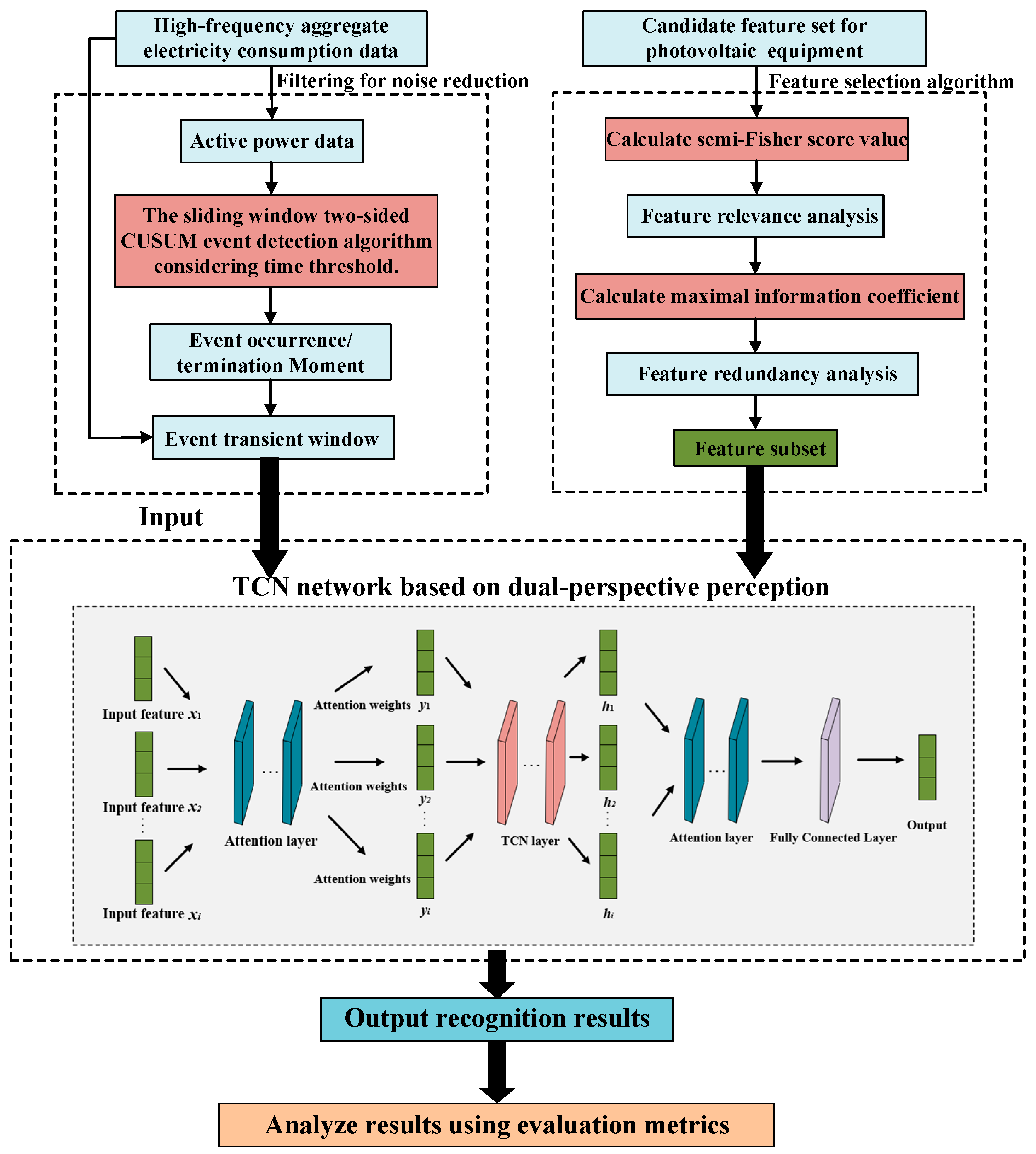
By using a feature selection method based on the semi-Fisher score and MIC, the discrimination and redundancy of nine types of transient features of PV systems were analyzed. The features were ranked, and a subset of PV device features with the highest classification accuracy was extracted.

(2)

To address the issue that current event detection algorithms are not suitable for detecting the power characteristics of PV devices, which have long rise times and large fluctuations, a sliding-window two-sided CUSUM event detection algorithm considering the time threshold was proposed. The Gaussian function, sigmoid function, and volatility criteria were utilized to accurately obtain real-time behavior time windows of PVs, enabling the real-time and accurate judgment of PV events.

(3)

A TCN model with attention mechanisms was proposed. Feature combination and balance weights were employed to accurately perceive and identify the behavior of residential PV systems. The effectiveness and superiority of the proposed method were validated using a custom-designed non-intrusive platform.

2. Non-Intrusive Residential PV Recognition Process

Figure 1 illustrates the overall process of the non-intrusive residential PV identification method proposed in this paper. It mainly includes four parts: high-frequency data acquisition, a transient feature selection method using the semi-Fisher score and MIC, event detection using a sliding window two-sided CUSUM algorithm considering the time threshold, and PV identification using the TCN model with attention mechanisms.

Firstly, focusing on the monitoring objective of the residential PV grid connection and control state switching, the discrimination and redundancy of different transient features in various devices are analyzed using the feature selection algorithm based on the semi-Fisher score and MIC, and the features are sorted accordingly. Secondly, the high-frequency active power data are used as input to the sliding-window two-sided CUSUM event detection algorithm considering the time threshold to accurately locate the occurrence and end time of various electrical events and extract the transient time windows of the original feature set of various devices. Then, the features are sequentially added to the feature subset based on the sorting results, and their transient time windows are the input to the TCN model with attention mechanisms. The network assigns weights to each feature and performs classification and identification. Finally, the proposed method is verified through multi-scene analysis on a custom-designed non-intrusive experimental platform.

3. Feature Selection and Ranking of PV Devices

3.1. Feature Analysis of PV Devices

With a wide variety of residential load types, residential PV devices exhibit unique characteristic quantities due to differences in their components, working principles, and operational modes. In this paper, the residential two-stage PV off-grid and control state switching was taken as the monitoring target, and its features were selected and analyzed. The PV system adopted a series–parallel structure for its centralized PV inverter, mainly including a single-phase PV inverter and a three-phase PV inverter two cases, and its structure and control block diagram are shown in Figure 2 and Figure 3 below. The PV was grid-connected with a unit power factor and was controlled by Maximum Power Point Tracking (MPPT) [35]; Perturbation and Observation (P&O), as a widely used MPPT control method, was adopted in this paper to realize maximum photovoltaic efficiency conversion, as shown in Figure 4. The PV array consisted of n PV cell modules in series and m PV cell modules in parallel, in order to improve the output capability of the modules under localized shading conditions; the cell units were grouped in parallel with bypass diodes, as shown in Figure 2. The power–voltage characteristics of a PV array will have multiple peaks when it is shaded by localized shadows, and heuristic algorithms or reconfigurable circuits and other methods have often been used in the literature to achieve global MPPT [36]. Although the traditional MPPT algorithms based on P&O in this paper may fall into the local optimum and, thus, reduce the PV output, the different MPPT algorithms have no effect on the feature selection and identification results in this paper.

This paper selected the nine types of transient process features as the initial feature set, as shown in

Table 1. Number and name of features.

Feature ID	Feature Name
A1	Active power
A2	Reactive power
A3	Current Amplitude
A4	Current Total Harmonic Distortion
A5	Current 3rd harmonic amplitude
A6	Current 5th harmonic amplitude
A7	Current 7th harmonic amplitude
A8	Current Pulse Peak
A9	Voltage amplitude

, during grid connection and state switching (the transient characteristics described in this paper are eigenvalues calculated from the sampling points during the transient). It is important to note that using a larger number of feature types does not necessarily improve recognition. Features with low discrimination can interfere with recognition, and feature sets with high redundancy increase computational costs without improving recognition accuracy. Therefore, it is necessary to select a subset of features with high discrimination and low redundancy as the basis for discrimination. Thus, this paper adopts a transient feature selection method based on semi-Fisher score and MIC to calculate and rank the discriminatory and redundancy of various transient features across different devices.

3.2. Semi-Fisher Score Method

The Fisher score is an effective criterion for evaluating the features of a given sample. Its main objective is to find a subset of features in the feature space that maximizes the distance between data points of different classes, while minimizing the distance between data points of the same class [37]. However, it should be noted that the standard Fisher score is applicable only when samples have complete and labeled classifications, making it a supervised feature selection method. In this paper, we focused on the identification of residential PV samples. These samples are were from the user’s residential wiring and included samples from various devices. However, only the samples belonging to the user’s PV device had accurate labels, resulting in a scenario of semi-supervised learning. In order to overcome this limitation, the concept of the semi-Fisher score was introduced [38]. It incorporates the exploration and utilization of both the global distribution information and the local structural information in the dataset. The formulation of the semi-Fisher score for semi-supervised feature selection can be stated as

$$F_s^r=\frac{{\displaystyle \sum _{i=1}^c{n}_i({\mu }_r^i-{\mu }_r}{)}^2+\delta V_r}{{\displaystyle \sum _{i=1}^c{n}_i{({\sigma }_r^i)}^2+\lambda \times J(f_r)}}$$

(1)

where n is the number of samples in the sample set, c is the number of categories in the samples, and m is the dimensionality of the sample features. c is the category index. n_i denotes the quantity of samples in the i-th class. μ_r is the mean value of all samples on the r-th feature. ${\mu }_r^i$, ${({\sigma }_r^i)}^2$ are the mean and variance of the r-th feature for samples in the i-th class. δ (where δ ≥ 0) and λ (where λ ≥ 0) are two control parameters. V_r is the variance score of the r-th feature, which measures the ability of the feature to preserve global distribution information. The definition of J(f_r) is

$$J(f_r)={\displaystyle \sum _{i,j}{(f_{ri}-f_{rj})}^2{W}_{ij}}$$

(2)

where f_ri and f_rj represent the r-th feature of the i-th and j-th samples, respectively. W is an n by n weight matrix. If the standard Euclidean distance between sample i and sample j is less than the average distance among the PV device samples, then the element W_ij is set to 1; otherwise, it is set to 0. This measures the capability of preserving local structural information. It can be observed that the semi-supervised Fisher score effectively utilizes both local structural and global distribution information inherent in all labeled and unlabeled samples, thereby evaluating features in the semi-supervised scenario.

3.3. MIC Method

The semi-Fisher score can assess the discrimination of features, but it cannot determine the redundancy of a feature set. The MIC can measure the linear or nonlinear correlation between two random variables, thereby quantifying the correlation between features [39]. A higher MIC value indicates a stronger correlation. In this study, the MIC method was used to measure the redundancy between sample features. The calculation method is as follows.

Given two sets of feature variables X = {x_i, i = 1,2,…,n} and Y = {y_i, i = 1,2,…,n}, where x_i and y_i represent the values of the x-th and y-th features of the i-th sample, and n represents the number of samples, the redundancy between X and Y can be calculated as

$$MIC(X,Y)=\underset{\left|X\right|\left|Y\right|<B}{\max }\frac{\max (I(X,Y))}{{\log }_2\min (\left|X\right|,\left|Y\right|))}$$

(3)

where B is the upper limit value of the grid division of size X × Y; it is a growing function related to the number of data samples, denoted as n. In reference [40], it is suggested to set B(n) = n^0.6 for better performance. I(X:Y) is the mutual information between X and Y, and it is defined as

$$I(X,Y)={\displaystyle \sum _{x\in X}{\displaystyle \sum _{y\in Y}p(x,y)\log \frac{p(x,y)}{p(x)p(y)}}}$$

(4)

where p(x,y) is the joint probability density of variables X and Y, whereas p(x) and p(y) is the marginal probability densities of X and Y, respectively.

3.4. Methods for Feature Selection and Ranking

In this paper, the maximum discrimination and minimum redundancy of the selected feature subset were taken as the objectives. In the first stage, the Fisher score value was calculated for each feature using the semi-Fisher score algorithm, and feature importance was ranked accordingly. In the second stage, the MIC was used to evaluate the redundancy between features. The feature with the highest importance and the lowest redundancy with the already-selected feature subset was sequentially chosen from the candidate features to join the subset. The procedures are defined as follows.

The first selected feature F₁ is

$$F_1=\underset{i}{\arg \max }(\alpha d_i-(1-\alpha )MI{C}_{\mathrm{average}}(F_i\cup F_{m-i}))$$

(5)

where d_i is the discrimination of the i-th feature, calculated using the aforementioned Equation (1). $MI{C}_{\mathrm{average}}(F_i\cup F_{m-i})$ is the average redundancy of the i-th feature with all other features, calculated using Equation (3); α is a weighting parameter.

The n-th selected feature F_n is

$$F_n=\underset{i}{\arg \max }(\alpha d_i-(1-\alpha )MI{C}_{\mathrm{average}}(F_i\cup F_s))$$

(6)

where F_s is the selected feature subset; $MI{C}_{\mathrm{average}}(F_i\cup F_s)$ is the average redundancy of the i-th feature with the features already selected in the subset.

4. Sliding-Window Two-Sided CUSUM Event Detection Algorithm Considering the Time Threshold

This paper utilized event detection algorithms to temporally locate the grid connection and state-switching behaviors of PV systems in order to extract their transient features. Due to the large magnitude and variability of active power in high-frequency total electricity data, this study employed active power as the detection signal. Based on the analysis of the power characteristics of PV systems [41], after PV devices start, they do not immediately enter a stable operating state. Instead, there is a prolonged and fluctuating climbing state during the variation process of active power characteristics. Therefore, in addition to accurately determining the timing of PV device connection and startup, it is necessary to accurately identify when the PV device enters a steady state to avoid misjudgment. On the other hand, as the steady-state power of PV devices is generally higher than that of other devices, its operational fluctuations can easily impact the judgment of smaller-power devices being connected. Therefore, this paper proposes a compound window two-sided CUSUM event detection algorithm that considers a time threshold based on the traditional two-sided CUSUM algorithm [10].

The traditional two-sided CUSUM algorithm involves setting two consecutive sliding windows, namely the mean calculation window W_m and the transient detection window W_d, for a random time series X = {x(k)} with k = 1,2,…. The window lengths are denoted as N_m and N_n, respectively. The detection process is illustrated in Figure 5. The algorithm calculates the power mean values, M_m and M_d, within the two windows, using the following formulas:

$$M_m=\frac{1}{m}{\displaystyle \sum _{j=k}^{k+N_m-1}P(j)}$$

(7)

$$M_d=\frac{1}{n}{\displaystyle \sum _{j=k+N_m}^{k+N_m+N_d-1}P(j)}$$

(8)

where k is the sampling points of the mean calculation window. The two-sided event cumulative sums are defined as $g_k^{+}$ and $g_k^{-}$, and their specific calculation formulas can be obtained as

$$\left\{\begin{array}{l}{g}_0^{+}=0\\ g_k^{+}=\max (0,g_{k-1}^{+}+X_k-(M_m+\beta )) \end{array}\right.$$

(9)

$$\left\{\begin{array}{l}{g}_0^{-}=0\\ g_k^{-}=\max (0,g_{k-1}^{-}-X_k-(M_m-\beta )) \end{array}\right.$$

(10)

where β is the externally introduced noise and d is the time delay factor; the initial values are set to 0. The cumulative sum threshold for event occurrence is denoted as h. When 0 < $g_k^{+}$ < h, let d = d + 1. If we calculate $g_k^{+}$ until $g_k^{+}$ > h, a positive event is determined to have occurred, and the occurrence time is obtained using the inverse transformation t = k − d. The calculation method for h is based on the principles illustrated in Figure 6, which can be derived as

$$h=({\Delta }_{\min }-\beta )T_{\max }$$

(11)

In the equation, T_max = N_maxT_s; N_max is the maximum allowable delay in terms of the number of sampling points, while T_s is the sampling interval, and β is associated with measurement noise.

Due to the long response time and high noise level of PV systems, as well as the higher power signal compared to other electrical devices, traditional two-sided CUSUM algorithms may suffer from issues such as false alarms and inaccurate judgments in capturing the PV action events. Therefore, this paper proposes a sliding window two-sided CUSUM event detection algorithm considering the time threshold. The workflow is illustrated in the following Figure 7.

Firstly, a time difference threshold method is introduced, where two consecutive events with a time difference within a certain time threshold are considered as a single event. The second event is treated as a false alarm and removed to alleviate the issue of false alarms, which can be derived as

$$T_w-T_{w-1}=\Delta t<T_{th}$$

(12)

where Δt is the time difference between two consecutive events, and T_th refers to the given time threshold. This threshold is determined based on the transient characteristics of various devices.

Next, a Gaussian function is applied to the average value window, and an appropriate σ value is selected to filter the data of the small-reference-value window before and after it to a certain extent. The representation of weight values using the Gaussian function is

$$f(u_i)=\frac{1}{\sigma \sqrt{2\pi }}{e}^{-\frac{(u_i-u_c)}{2{\sigma }^2}}$$

(13)

where u_i is each sampling point in the average value window, and u_c is the position of the sampling point in the middle of the window. Normalizing f(u_i), we obtain the weight value φ(u_i)

$$\phi (u_i)=\frac{f(u_i)}{{\displaystyle \sum _{u_i=k}^{k+N_m}f(u_i)}}$$

(14)

The average value μ_gauss of the obtained Gaussian window is

$${\mu }_{gauss}={\displaystyle \sum _{u_i=k}^{k+N_m}\phi (u_i)}{W}_m(u_i)$$

(15)

The detection window needs to consider both anti-noise characteristics and sensitivity to transient events. In the detection process, the cumulative weight of the initial segment of the detection window, which is easily affected by noise, is reduced, while the weight of the sampling values that show a continuous increase in climbing events is gradually increased. This can improve the detection accuracy, so an improved Sigmoid function is used to modify the detection window, whose expression is

$$h(v_i)=\frac{1}{1+e^{-\alpha (v_i-u_d)}}$$

(16)

where μ_d is the middle value of the maximum width of the detection window, and α is the coefficient for backward offset of the detection window weight. Normalizing h(v_i), we obtain

$$\psi (v_i)=\frac{h(v_i)}{{\displaystyle \sum _{v_i=k+N_m}^{k+N_m+N_d}h(v_i)/N_d}}$$

(17)

$g_k^{+}$, $g_k^{-}$ are, respectively, represented as

$$\left\{\begin{array}{l}{g}_0^{+}=0\\ g_k^{+}=\max (0,g_{k-1}^{+}+\psi (v_i)M_d-({\mu }_{guass}+\beta )) \end{array}\right.$$

(18)

$$\left\{\begin{array}{l}{g}_0^{-}=0\\ g_k^{-}=\max (0,g_{k-1}^{-}-\psi (v_i)M_d+({\mu }_{guass}-\beta )) \end{array}\right.$$

(19)

M_d is represented as:

$$M_d=\frac{1}{N_d}{\displaystyle \sum _{v_i=k+N_m}^{k+N_m+N_d}{W}_d}(v_i)$$

(20)

For determining the moment of entering a steady state, if the cumulative sum of events is greater than h, it indicates that an event has occurred. At this point, further assessment is required.

$$g_{k+1}-g_k\le {\Delta }_{\min }$$

(21)

If the above condition is met, it is judged that the system has entered a steady state. The sliding window then reads the next data block. If the condition is not met, the process continues in a loop until the condition is satisfied.

Finally, as PVs are high-power devices, fluctuations in their operating power can easily affect the normal operation of smaller-power devices when they connect or disconnect. Therefore, a judging mechanism is set to determine whether there are similar-magnitude power fluctuations before a sharp increase or decrease in power occurs, using the similarity of fluctuations. The judging condition is expressed in the following equation:

$$u=g_{w+1}-g_w$$

(22)

$$\left|g_{w-i+1}-g_{w-i}-u\right|\le eu\hspace{1em}i=0,1,2,3$$

(23)

where $g_w$ is the cumulative sum within a window, and e is the similarity coefficient. If the above condition is not met, it indicates that there is no similar magnitude power fluctuation detected before the observed power increase or decrease, implying that the power fluctuation is not due to the operating fluctuations of the high-power device in operation.

5. Identification Model of TCN with Attention Mechanisms

Based on the feature selection method using the semi-Fisher score and MIC, as described in Section 3.4, the discrimination and redundancy of different transient features in various devices were computed and ranked. According to the ranking results, the features were added to the feature subset in order, and then the transient time series of various types of features were obtained as model inputs by using the event detection algorithm, to which the paper introduced the attention mechanisms to measure various types of feature inputs, and TCN neural network has strong feature extraction and fusion capabilities [42]. Based on these considerations, this paper proposes the recognition model of the TCN model with attention mechanisms.

5.1. Concatenated Attention Mechanism

The attention mechanism is a resource allocation mechanism proposed to simulate how the human brain allocates attention to external information. It assigns different weights to different input features to emphasize more important features, thereby improving model accuracy without increasing computational and storage costs [43]. In this paper, the attention mechanism is utilized to concatenate feature inputs of different characteristics [44].

For feature vectors ${\overrightarrow{h}}_i,{\overrightarrow{h}}_j$, firstly, a linear transformation is applied to them using the weight matrix W. Then, perform self-attention on feature vectors—a shared attentional mechanism $\overrightarrow{a}$ computes attention coefficients. Finally, softmax normalization is employed to compute the coefficient ${\alpha }_{ij}$, as shown in the following equation. The computation process is illustrated in Figure 8a.

$${\alpha }_{ij}=\frac{\exp (Leaky\mathrm{Re}LU({\overrightarrow{a}}^T[\left.W{\overrightarrow{h}}_i\right|\left|W{\overrightarrow{h}}_j]))\right.}{{\displaystyle {\sum }_{j\in N_i}\exp (Leaky\mathrm{Re}LU({\overrightarrow{a}}^T[\left.W{\overrightarrow{h}}_i\right|\left|W{\overrightarrow{h}}_j]))\right.}}$$

(24)

where T represents transposition and || is the concatenation operation. The attention mechanism a is a single-layer feedforward neural network, parametrized by a weight vector $\overrightarrow{a}\in R^{2F^{\prime }}$, and applying the LeakyReLU nonlinearity.

Then, the linear combination is performed between the corresponding features and their attention coefficients. The resulting feature vectors are concatenated, and eventually outputted, as shown in the following equation. The computation process is illustrated in Figure 8b.

$${\overrightarrow{h}}_i^{\prime }=\sigma (\frac{1}{K}{\displaystyle \sum _{k=1}^K{\displaystyle \sum _{j\in N_i}{a}_{ij}^k{W}^k{\overrightarrow{h}}_j}})$$

(25)

In the equation, $\sigma$ is the non-linear coefficient, $a_{ij}^k$ are normalized attention coefficients computed by the k-th attention mechanism, $W^k$ is the corresponding input linear transformation’s weight matrix, and N is the number of feature values.

5.2. Temporal Convolutional Network

TCN is an advanced variant of convolutional neural networks (CNNs) that incorporates dilated causal convolution (DCC) to capture long-term dependencies and effectively model sequence data [42]. Furthermore, TCN employs residual blocks to alleviate the issue of vanishing gradients and promote information flow within the network [45]. The inclusion of residual blocks allows the network to bypass specific layers and propagate residual information, effectively addressing the common problem of degradation in deep neural networks.

(1)

TCN Model

For a time series input $x_0,\cdot \cdot \cdot ,x_t$, the corresponding predicted output is ${\widehat{y}}_0,\cdot \cdot \cdot ,{\widehat{y}}_t$. The relationship between the input and output sequences can be described as

$${\widehat{y}}_0,\cdot \cdot \cdot ,{\widehat{y}}_t=f(x_0,\cdot \cdot \cdot ,x_t)$$

(26)

This equation implies that elements in the output sequence can only depend on elements that precede them in the input sequence. Causal convolution is a strict time-constrained structure that is unidirectional rather than bidirectional. The objective of sequence modeling is to find a network f that minimizes the expected loss between the actual output and the predicted output.

(2)

Dilated Causal Convolution

TCN is based on a 1D fully convolutional network and incorporates the advantages of causal convolution’s non-recurrent structure, allowing for the parallel input of time series data and a faster training speed. However, causal convolution increases the depth of the network significantly when dealing with large-scale time series data. To address this issue, TCN employs a series of dilated convolutions, as shown in Figure 9. By exponentially increasing the dilation factor, denoted as d, TCN effectively increases the receptive field of the network in proportion to its depth. For an input x and convolution kernel size $f:\{0,1,2,\dots ,k-1\}$, the dilated convolution operation F for a time series s can be represented as

$$F(s)=(x\ast f_d)(s)={\displaystyle \sum _{i=0}^{k-1}f(i)x_{s-d\cdot i}}$$

(27)

where K represents the specific value of the convolution kernel, and $x_{s-d\cdot i}$ is the product of the step lengths of all previous layers.

(3)

Residual Block

The residual block is another important component of the TCN model, which mitigates the issues of gradient vanishing and degradation during deep learning training through Skip Connection operations [42]. The output of the residual block depends on the input and a series of transformations Ψ, and it is defined as follows:

$$O_{block}=Activation(x_{block}+\psi (x_{block}))$$

(28)

where $x_{block}$ represents the input value, F(x) represents the output value, Activation is the Activation function, and $O_{block}$ is the output value of the residual block. The residual block structure is shown in Figure 10. Overall, TCN combines the advantages of capturing long-range dependencies with DCC and the characteristics of residual blocks to prevent network degradation, thereby effectively improving the capability and robustness of feature extraction in the model.

5.3. Framework of TCN Model with Attention Mechanisms

The proposed TCN model with the attention mechanism in this paper includes multiple feature inputs, two attention layers, one TCN layer, fully connected layers, and output classification values. The input feature vectors {x₁, x₂,…, x_i} are first used in the first attention layer to calculate the weight vectors. The weight vectors are then concatenated with the input vectors of the current layer to obtain new vectors {y₁, y₂, …, y_i}. Next, the vectors go through the TCN layer for convolutional processing, followed by the attention layer to repeat the concatenation and weight calculation operations. Finally, the vectors are fed into the fully connected layers to compute the classification values. The attention mechanism is introduced before and after the TCN layer to improve the identification efficiency through the weight assignment process. The attention-based TCN model is illustrated in Figure 11.

6. Example Verification and Analysis

6.1. Hardware Environment and Experimental Platform

This paper implemented the above-mentioned model using the PyTorch deep learning framework. The training and testing were performed on a computing platform with an Intel Core i5-8265U CPU, Intel, Santa Clara, CA, USA, 8 GB of memory, and an NVIDIA GeForce GTX 1080 GPU (Nvidia, Santa Clara, CA, USA) with 11 GB of memory.

6.2. Data Set Selection

Due to the lack of high-frequency electrical data for PV components in existing datasets, we built a non-intrusive experimental platform for data collection, processing, and storage. The data acquisition device synchronously collected high-frequency voltage and current data at the residential entrance bus. The detailed information of residential appliances, simulated for the experiment, is listed in

Table 2. Information on equipment used for experimental sampling.

Equipment Type	Brand Model	Rated Power/kW
PV equipment	CHINT CPS SCA36KTL-DO-480, Chint Power Systems America, Richardson, TX, USA	5
Air conditioner	Gree RF7.2WQ/NhA-N3JY01, Gree Electric, Zhuhai, China	2
Electric kettle	PHILIPS HD9316, Philips, Amsterdam, The Netherlands	1.8
Microwaves	GalanZ G80F23CN2P-B5(RO), Galanz, Foshan, China	1.5
Refrigerator	Hisense BCD-183FH, Hisense, Qingdao, China	0.52
Lighting	OPPLE, Suzhou, China	0.1

. The platform was based on a three-layer interfacing and data-acquisition device using the DSP TMS320F28335, Texas Instruments, Dallas, TX, USA. The voltage sensor model was LV25-P/SP5, the current sensor model was ZQM150LTBS, and the sampling frequency was set to 1000 Hz. Software tools such as Code Composer Studio 6.0 were employed for high-frequency signal filtering and AD sampling. The sampled dataset included time, three-phase voltage, current, current harmonics, active power, and reactive power. The platform architecture is shown in Figure 12.

Since this paper focused only on the identification of PV devices, in the data sampling process, to maintain the platform under normal lighting conditions (including occasional photovoltaic received localized shadow blocking during the conditions), all the types of normal-access equipment, to confirm that the overall test system was operating normally, recorded the grid-connected-containing single-phase and three-phase photovoltaic and the control state of the switching of the time data, and these events were marked as PV events. Other devices, considered as disturbances, were randomly switched on during the sampling process without specific event labeling; their activation times were recorded. The dataset consisted of nearly 1500 events and around 300 PV events, which were used to evaluate the event detection and PV device identification methods. The entire dataset was randomly partitioned into an 80% training dataset and a 20% testing dataset.

6.3. Evaluation Indicators

In order to evaluate the accuracy of the proposed identification approach for residential PV systems using transient features and TCN with attention mechanisms, as well as the accuracy of the sliding-window two-sided CUSUM event detection algorithm, considering the time threshold for electrical-event detection and the precision of capturing the event time window, several commonly used performance metrics in this type of problem were selected.

Precision rate: this represents the proportion of correctly classified events among all detected events. Recall indicates the proportion of all events that are detected. The calculation formula is as follows:

$$P_{precision}=\frac{TP}{TP+FP}$$

(29)

$$P_{recall}=\frac{TP}{TP+FN}$$

(30)

In the formulas, TP represents true positive, which is the number of positive samples correctly classified as positive; FP represents false positive, which is the number of negative samples incorrectly classified as positive; and FN represents false negative, which is the number of positive samples incorrectly classified as negative.

The F_1-score is the harmonic mean of precision and recall. The calculation formula is as follows:

$$F_{1-score}=\frac{2\times P_{precision}\times P_{recall}}{P_{precision}+P_{recall}}$$

(31)

The time error mean indicates the precision of the event detection algorithm in calculating the time of occurrence of an event.

$$T_{MAE}=\frac{1}{n}{\displaystyle \sum _{i=1}^n\left|t_i-t_{i,real}\right|}$$

(32)

where n is the number of events detected, t_i is the event occurrence time calculated by the event detection algorithm, and t_i,real is the real occurrence time of the event.

6.4. Validation of Event Detection Performance

To validate the proposed sliding window two-sided CUSUM event detection algorithm considering the time threshold, the collected one-dimensional power series from the electricity meter was used as the input. The algorithm was compared with BIC, Hotelling T², and the traditional CUSUM algorithm. The actual power series of the selected dataset in this article is shown in Figure 13.

According to the actual debugging situation, the relevant parameters were set as follows: the window length for calculating the average value was N_m = 8, the window length for transient process detection was N_d = 12, the noise parameter β was 50, the threshold value h was 500, σ was 1.2, α was 1, and $\lambda$ was 0.2. The specific results of various event detection algorithms are shown in

Table 3. Results of various event detection algorithms.

	BIC	Hotelling T2	CUSUM	Improved CUSUM
PR	0.889	0.729	0.946	0.976
Recall	0.891	0.965	0.912	0.985
F1	0.890	0.831	0.929	0.980
TMAE/s	0.328	0.456	0.147	0.029

. Based on the above statistical results, it can be concluded that the algorithm proposed in this paper, which utilizes the time threshold, power fluctuation criterion, and weighted composite window, can improve the accuracy of event detection compared to other algorithms, and accurately record the start and end positions of transient events. Figure 14a and Figure 14b, respectively, display the change in the total power of the electricity meter and the cumulative sum of the corresponding event detection algorithm during a certain grid-connected moment of the PV equipment, which show the calculation process of the detection algorithm in detail.

6.5. Validation of Feature Selection and Ranking Methods

According to the measurement results of the discrimination and redundancy of different features from various devices using the semi-Fisher score and MIC feature selection methods, the features were sorted according to Equation (9) with a parameter α of 0.5. Based on the sorting results, the features were sequentially added to the feature subset. Using the event detection algorithm mentioned earlier to record the start and end positions of various events, the feature quantities of the feature subset were extracted around the starting positions using a time window of length 200. The transient feature quantities in each window were then input into a TCN with attention mechanisms. To demonstrate the effectiveness of the feature selection method proposed in this paper, the test results were compared with traditional mRMR and reliefF methods, as shown in Figure 15. The accuracy of identification represents the proportion of correctly classified samples to the total number of test samples.

In Figure 15a, the horizontal axis represents the importance order of nine features, where the importance decreases from left to right. The vertical axis represents the identification accuracy corresponding to adding the features in the horizontal axis sequentially to the feature subset. It can be observed that as the number of features increases, the accuracy of PV-device identification gradually improves. When the 4th feature is added, the identification accuracy reaches its highest point. However, with the subsequent addition of features, the identification accuracy decreases, indicating that adding features with lower importance actually leads to a decrease in identification accuracy. Among them, the maximum identification correctness is 98.23% when four features, namely, the active power, current amplitude, current crest factor, and current 7th harmonic amplitude, are selected as feature subsets. Therefore, this feature subset represents the optimal subset for identification.

By comparing Figure 15a–c, it can be concluded that the feature selection method proposed in this study not only improves the accuracy of identification but also greatly reduces the dimensionality of the features. Compared to other methods, it offers the advantage of lower computational complexity.

6.6. Validation of Classification Algorithms

To verify the effectiveness of the TCN model with attention mechanisms, it was compared with a OneClass support vector machine (OCSVM), CNNs, long short-term memory (LSTM), gated recurrent unit (GRU), and backpropagation (BP) neural network algorithms. The comparative results are shown in

Table 4. Comparison of recognition effect of different algorithms.

Algorithm	Identification Accuracy/%	Number of Feature Subsets
TCN model with attention mechanisms	98.32	4
GRU	92.21	6
LSTM	93.06	6
CNNs	93.45	5
BP	91.83	5
OCSVM	86.23	6

.

From Table 4, it can be observed that the One-Class support vector machine (OCSVM) algorithm had the lowest identification accuracy and required the highest number of features, and the identification accuracy of other neural network algorithms was also not high. The TCN algorithm with the attention mechanism outperformed other algorithms in terms of identification accuracy and required fewer features for identification, reducing the feature dimensionality and computational costs.

7. Conclusions

This paper introduced a non-intrusive method for identifying residential PV systems using transient features, leveraging the TCN model with attention mechanisms, and the method was validated using real measurement data. The results demonstrate that the transient feature selection method of the semi-Fisher Score and MIC in this paper can fully exploit the information of unlabeled samples and select the subset of features (active power, current amplitude, current crest factor, and current 7th harmonic amplitude) with the best identification effect compared with the traditional mRMR and reliefF feature selection methods, effectively reducing the feature dimension and computational cost of the identification. In addition, the TCN model with attention mechanisms gave different weights to multi-input features through the attention mechanism to highlight the more critical features, which greatly improved the accuracy of the discrimination to 98.23% compared with LSTM, GRU, CNNs, OCSVM, and BP. The sliding-window two-sided CUSUM event detection algorithm considering the time threshold not only improves the precision rate and recall rate of event detection, but also can accurately locate the PV grid connection and state-switching behaviors in real time. The results show that the mean error of the temporal localization of the algorithm was 0.029 s, which was a reduction of 0.2 s compared with the other algorithms, which further verifies the high efficiency of the analytical methods and algorithms in this paper. Future research will focus on enhancing the learning speed of the algorithms for practical applications. Additionally, factors such as temperature, humidity, real-time electricity prices, and user habits will also be taken into account to further improve the accuracy of the model. Meanwhile, the method of this paper can also be generalized and applied to other special or abnormal load monitoring.

References

1. United Nations Climate Change. The Paris Agreement. Available online: https://unfccc.int/process-and-meetings/the-paris-agreement/the-paris-agreement (accessed on 21 March 2021).
2. Jäger-Waldau, A. Snapshot of photovoltaics—March 2021. EPJ Photovolt. 2021, 12, 7. [Google Scholar] [CrossRef]
3. Mahato, G.C.; Choudhury, T.R.; Nayak, B.; Debnath, D.; Santra, S.B.; Misra, B. A review on high PV penetration on smart grid: Challenges and its mitigation using FPPT. In Proceedings of the 2021 1st International Conference on Power Electronics and Energy (ICPEE), Bhubaneswar, India, 2–3 January 2021; pp. 1–6. [Google Scholar]
4. Amanipoor, A.; Golsorkhi, M.S.; Bayati, N.; Savaghebi, M. V-Iq Based Control Scheme for Mitigation of Transient Overvoltage in Distribution Feeders with High PV Penetration. IEEE Trans. Sustain. Energy 2022, 14, 283–296. [Google Scholar] [CrossRef]
5. Li, Y.; Wang, R.; Yang, Z. Optimal Scheduling of Isolated Microgrids Using Automated Reinforcement Learning-Based Multi-Period Forecasting. IEEE Trans. Sustain. Energy 2022, 13, 159–169. [Google Scholar] [CrossRef]
6. Hart, G.W. Nonintrusive appliance load monitoring. Proc. IEEE 1992, 80, 1870–1891. [Google Scholar] [CrossRef]
7. Luo, D.; Norford, L.; Shaw, S.; Leeb, S.; Ashrae, T. Monitoring HVAC equipment electrical loads from a centralized location-methods and field test results. ASHRAE Trans. 2002, 108, 841–857. [Google Scholar]
8. De Baets, L.; Ruyssinck, J.; Develder, C.; Dhaene, T.; Deschrijver, D. On the Bayesian optimization and robustness of event detection methods in NILM. Energy Build. 2017, 145, 57–66. [Google Scholar] [CrossRef]
9. Ajmera, J.; McCowan, I.; Bourlard, H. Robust speaker change detection. IEEE Signal Process. Lett. 2004, 11, 649–651. [Google Scholar] [CrossRef]
10. Lin, S.; Zhao, L.; Li, F.; Liu, Q.; Li, D.; Fu, Y. A nonintrusive load identification method for residential applications based on quadratic programming. Electr. Power Syst. Res. 2016, 133, 241–248. [Google Scholar] [CrossRef]
11. Truong, C.; Oudre, L.; Vayatis, N. Selective review of offline change point detection methods. Signal Process. 2019, 167, 107299. [Google Scholar] [CrossRef]
12. Cominola, A.; Giuliani, M.; Piga, D.; Castelletti, A.; Rizzoli, A. A Hybrid Signature-based Iterative Disaggregation algorithm for Non-Intrusive Load Monitoring. Appl. Energy 2017, 185, 331–344. [Google Scholar] [CrossRef]
13. Lindahl, P.A.; Ali, M.T.; Armstrong, P.; Aboulian, A.; Donnal, J.; Norford, L.; Leeb, S.B. Nonintrusive Load Monitoring of Variable Speed Drive Cooling Systems. IEEE Access 2020, 8, 211451–211463. [Google Scholar] [CrossRef]
14. Liu, Y.C.; Wang, X.; You, W. Non-intrusive load monitoring by voltage-current trajectory enabled transfer learning. IEEE Trans. Smart Grid 2019, 10, 5609–5619. [Google Scholar] [CrossRef]
15. Tayal, A.; Dewan, L.; Lather, J.S. Artificial neural network based source identification producing harmonic pollution in the electric network. In Advances in Renewable Energy and Sustainable Environment; Dewan, L., Bansal, R.C., Kalla, U.K., Eds.; Springer: Singapore, 2021; pp. 49–58. [Google Scholar]
16. Lee, D. Phase noise as power characteristic of individual appliance for non-intrusive load monitoring. Electron. Lett. 2018, 54, 993–995. [Google Scholar] [CrossRef]
17. Drouaz, M.; Colicchio, B.; Moukadem, A.; Dieterlen, A.; Ould-Abdeslam, D. New Time-Frequency Transient Features for Nonintrusive Load Monitoring. Energies 2021, 14, 1437. [Google Scholar] [CrossRef]
18. Hernandez, A.S.; Ballado, A.H.; Heredia, A.P.D. Development of a non-intrusive load monitoring (NILM) with unknown loads using support vector machine. In Proceedings of the 2021 IEEE International Conference on Automatic Control & Intelligent Systems (I2CACIS), Shah Alam, Malaysia, 26 June 2021; pp. 203–207. [Google Scholar] [CrossRef]
19. Dufour, L.; Genoud, D.; Jara, A.; Treboux, J.; Ladevie, B.; Bezian, J.-J. A non-intrusive model to predict the exible energy in a residential building. In Proceedings of the 2015 IEEE Wireless Communications and Networking Conference Workshops (WCNCW), New Orleans, LA, USA, 9–12 March 2015; pp. 69–74. [Google Scholar] [CrossRef]
20. Wu, X.; Gao, Y.; Jiao, D. Multi-Label Classification Based on Random Forest Algorithm for Non-Intrusive Load Monitoring System. Processes 2019, 7, 337. [Google Scholar] [CrossRef]
21. Yang, C.C.; Soh, C.S.; Yap, V.V. A systematic approach in load disaggregation utilizing a multi-stage classification algorithm for consumer electrical appliances classification. Front. Energy 2019, 13, 386–398. [Google Scholar] [CrossRef]
22. Kelly, J.; Knottenbelt, W.J. Neural NILM: Deep Neural Networks Applied to Energy Disaggregation; Springer International Publishing: Cham, Switzerland, 2015. [Google Scholar]
23. Garcia-Perez, D.; Perez-Lopez, D.; Diaz-Blanco, I.; Gonzalez-Muniz, A.; Dominguez-Gonzalez, M.; Vega, A.A.C. Fully-Convolutional Denoising Auto-Encoders for NILM in Large Non-Residential Buildings. IEEE Trans. Smart Grid 2021, 12, 2722–2731. [Google Scholar] [CrossRef]
24. Çimen, H.; Wu, Y.; Wu, Y.; Terriche, Y.; Vasquez, J.C.; Guerrero, J.M. Deep learning-based probabilistic autoencoder for residential energy disaggregation: An adversarial approach. IEEE Trans. Ind. Inform. 2022, 18, 8399–8408. [Google Scholar] [CrossRef]
25. Norford, L.K.; Leeb, S.B. Non-intrusive electrical load monitoring in commercial buildings based on steady-state and transient load-detection algorithms. Energy Build. 1996, 24, 51–64. [Google Scholar] [CrossRef]
26. Enríquez, R.; Jiménez, M.; Heras, M. Towards non-intrusive thermal load Monitoring of buildings: BES calibration. Appl. Energy 2017, 191, 44–54. [Google Scholar] [CrossRef]
27. Xiang, Y.; Liu, J.; Li, R.; Li, F.; Gu, C.; Tang, S. Economic planning of electric vehicle charging stations considering traffic constraints and load profile templates. Appl. Energy 2016, 178, 647–659. [Google Scholar] [CrossRef]
28. Dinesh, C.; Welikala, S.; Liyanage, Y.; Ekanayake, M.P.B.; Godaliyadda, R.I.; Ekanayake, J. Non-intrusive load monitoring under residential solar power influx. Appl. Energy 2017, 205, 1068–1080. [Google Scholar] [CrossRef]
29. Jaramillo, A.F.M.; Laverty, D.M.; Rincon, J.M.D.; Brogan, P.; Morrow, D.J. Non-intrusive load monitoring algorithm for PV identification in the residential sector. In Proceedings of the 31st Irish Signals and Systems Conference (ISSC), Letterkenny, Ireland, 11–12 June 2020. [Google Scholar]
30. Jaramillo, A.M.F.; Lopez-Lorente, J.; Laverty, D.M. Effective identification of distributed energy resources using smart meter net-demand data. IET Smart Grid 2022, 5, 120–135. [Google Scholar] [CrossRef]
31. Vavouris, A.; Garside, B.; Stankovic, L.; Stankovic, V. Low-Frequency Non-Intrusive Load Monitoring of Electric Vehicles in Houses with Solar Generation: Generalisability and Transferability. Energies 2022, 15, 2200. [Google Scholar] [CrossRef]
32. Zhang, Y.; Qian, W.; Ye, Y.; Li, Y.; Tang, Y.; Long, Y.; Duan, M. A novel non-intrusive load monitoring method based on ResNet-seq2seq networks for energy disaggregation of distributed energy resources integrated with residential houses. Appl. Energy 2023, 349, 121703. [Google Scholar] [CrossRef]
33. Liu, Y.; Liu, C.; Ling, Q.; Zhao, X.; Gao, S.; Huang, X. Toward smart distributed renewable generation via multi-uncertainty featured non-intrusive interactive energy monitoring. Appl. Energy 2021, 303, 117689. [Google Scholar] [CrossRef]
34. Sun, Q.; Liu, Y.; Hu, J.; Hu, X. Non-intrusive We-energy Modeling Based on GAN Technology. Proc. CSEE 2020, 40, 6784–6794. [Google Scholar] [CrossRef]
35. Murtaza, A.F.; Sher, H.A. A Reconfiguration Circuit to Boost the Output Power of a Partially Shaded PV String. Energies 2023, 16, 622. [Google Scholar] [CrossRef]
36. Murtaza, A.F.; Sher, H.A.; Khan, F.U.; Nasir, A.; Spertino, F. Efficient MPP Tracking of Photovoltaic (PV) Array Through Modified Boost Converter With Simple SMC Voltage Regulator. IEEE Trans. Sustain. Energy 2022, 13, 1790–1801. [Google Scholar] [CrossRef]
37. Tsuda, K.; Kawanabe, M.; Müller, K.R. Clustering with the fisher score. In Proceedings of the Advances in Neural Information Processing Systems 15, NIPS 2002, Vancouver, BC, Canada, 9–14 December 2002; pp. 745–752. [Google Scholar]
38. Yang, M.; Chen, Y.; Ji, G. Semi-Fisher Score: A Semi-Supervised Method for Feature Selection//Proc of International Conference on Machine Learning and Cybernetics; IEEE Press: Piscataway, NJ, USA, 2010; pp. 527–532. [Google Scholar]
39. Reshef, Y.A.; Reshef, D.N.; Finucane, H.K.; Sabeti, P.C.; Mitzenmacher, M. Measuring dependence powerfully and equitably. J. Mach. Learn. Res. 2016, 17, 7406–7468. [Google Scholar]
40. Reshef, D.N.; Reshef, Y.A.; Finucane, H.K.; Grossman, S.R.; McVean, G.; Turnbaugh, P.J.; Lander, E.S.; Mitzenmacher, M.; Sabeti, P.C. Detecting Novel Associations in Large Data Sets. Science 2011, 334, 1518–1524. [Google Scholar] [CrossRef] [PubMed]
41. Romero-Cadaval, E.; Spagnuolo, G.; Franquelo, L.G.; Ramos-Paja, C.A.; Suntio, T.; Xiao, W.M. Grid-Connected Photovoltaic Generation Plants: Components and Operation. IEEE Ind. Electron. Mag. 2013, 7, 6–20. [Google Scholar] [CrossRef]
42. Bai, S.; Kolter, J.; Koltun, V. An Empirical Evaluation of Generic Convolutional and Recurrent Networks for Sequence Modelling [EB/OL]. Available online: https://arxiv.org/abs/1803.01271v1 (accessed on 16 May 2018).
43. Vaswani, A.; Shazeer, N.; Parmar, N.; Uszkoreit, J.; Jones, L.; Gomez, A.N.; Kaiser, Ł.; Polosukhin, I. Attention is all you need. In Proceedings of the Advances in Neural Information Processing Systems 30 (NIPS 2017), Long Beach, CA, USA, 4–9 December 2017. [Google Scholar]
44. Veličković, P.; Cucurull, G.; Casanova, A.; Romero, A.; Lio, P.; Bengio, Y. Graph Attention Networks. In Proceedings of the International Conference on Learning Representations (ICLR), Vancouver, BC, Canada, 30 April–3 May 2018. [Google Scholar]
45. He, K.; Zhang, X.; Ren, S.; Sun, J. Deep residual learning for image recognition [EB/OL]. 2015. Available online: https://arxiv.org/abs/1512.03385 (accessed on 25 August 2023).
Figure 1. The overall process of the PV identification system.
Sustainability 15 14865 g001
Figure 2. Photovoltaic-array system circuit: schematic.
Sustainability 15 14865 g002
Figure 3. Two-stage PV grid-connected control block diagram.
Sustainability 15 14865 g003
Figure 4. Perturbation observation method.
Sustainability 15 14865 g004
Figure 5. Schematic of the position of the sliding window during the event detection process.
Sustainability 15 14865 g005
Figure 6. Calculation of cumulative threshold.
Sustainability 15 14865 g006
Figure 7. Event detection algorithm flow.
Sustainability 15 14865 g007
Figure 8. Splice attention mechanism calculation process. (a) Process of calculating the coefficient of attentional mechanism. (b) Output feature calculation.
Sustainability 15 14865 g008
Figure 9. Expanding causal convolutional structures.
Sustainability 15 14865 g009
Figure 10. TCN network and TCN residual blocks.
Sustainability 15 14865 g010
Figure 11. TCN model with attention mechanisms.
Sustainability 15 14865 g011
Figure 12. Non-intrusive data acquisition platform.
Sustainability 15 14865 g012
Figure 13. Time-series meter-power diagram.
Sustainability 15 14865 g013
Figure 14. (a) PV grid-connected moment-meter power diagram. (b) Composite-window cumulative sum.
Sustainability 15 14865 g014
Figure 15. (a) The identification results obtained using the feature selection method based on the semi-Fisher score and MIC. (b) The identification results obtained using the reliefF method. (c) The identification results obtained using the mRMR method.
Sustainability 15 14865 g015