Article

District Heating for Poorly Insulated Residential Buildings—Comparing Results of Visual Study, Thermography, and Modeling

by
Stanislav Chicherin
1,2,*,
Andrey Zhuikov
3 and
Lyazzat Junussova
4
1
Thermo and Fluid Dynamics (FLOW), Faculty of Engineering, Vrije Universiteit Brussel (VUB), 1050 Brussels, Belgium
2
Brussels Institute for Thermal-Fluid Systems and Clean Energy (BRITE), Vrije Universiteit Brussel (VUB) and Université Libre de Bruxelles (ULB), 1050 Brussels, Belgium
3
Educational and Scientific Laboratory, Siberian Federal University, Krasnoyarsk 660041, Russia
4
Institute of Heat Power Engineering and Control Systems, Almaty University of Power Engineering and Telecommunications (AUPET), 050013 Almaty, Kazakhstan
*
Author to whom correspondence should be addressed.
Sustainability 2023, 15(20), 14908; https://doi.org/10.3390/su152014908
Submission received: 21 September 2023 / Revised: 8 October 2023 / Accepted: 10 October 2023 / Published: 16 October 2023
(This article belongs to the Special Issue Advances in Sustainable Energy Technologies)

Abstract

:
Newer buildings have a lower but smoother profile of indoor temperature, while older buildings are less energy efficient. Sometimes, the indoor temperature is unreasonably high, being 25–30 °C. There are buildings where the indoor temperature does not correlate with the outdoor one. Correction factors adjusting convective heat transfer coefficients are suggested. Energy demand is defined using the rate of heat loss and internal heat gains for the given building construction and design consumption profile. We suggest adjusting the setpoints of the secondary supply temperature to keep indoor and return temperatures lower. Correcting a traditional approach when designing a building may minimize energy consumption by 23.3% and increase the annual performance by up to 14.1%. The reductions of thermal peak resulting from a new type of controller adjustment (for instance, discrete) compared to the traditional operation range from roughly 10 to 30%, respectively. A better understanding of the system operation is a necessary step to switch to fourth-generation district heating (4GDH). This methodology is especially helpful in shaving daily peaks of heat demand. Building envelopes ease the charging, maximum storage capacity, and balance of the given generation and demand profiles, which are key factors in achieving the reduction in greenhouse gas (GHG) emissions. Once the heat demand is covered according to the maximum storage capacity for the given generation and demand profile, fewer efforts to modernize a district heating network are required.

1. Introduction

Excluding demand-side measures, there are other ways of suggesting optimal strategies for the management of district heating (DH) systems. In [1], both temperature boosting and thermal energy storage are considered. The capacity of a typical short-term energy storage of a hot water buffer tank is usually up to 50 MWh. In [2], the sum of the energy absorbed by the distribution system, the district heating (DH) substations, space heating (SH) systems, and radiators, and the energy released by the sensible heat accumulator are 10 times higher—330 and 440 MWh, respectively.
In [3], the system is preheated well before the outdoor temperature is expected to decrease below the design outdoor temperature (DOT). This results in continuous transient processes and is associated with errors, meaning the DH network should not be ignored as a thermal accumulator. Therefore, our novelty is that we begin our research from the study of operational profiles on a primary side of the DH system; these operational profiles have already taken all the transient processes into account. Some methodologies are able to detect peaks happening due to the transient behavior [4] or internal heat gains [5].
In [6], an office building is modeled and simulated in TRNSYS, inputting the solar radiation and weather data from the local meteorological station. In the heat supply, flexibility is typically created by temporarily increasing the supply temperature [7]. Sun et al. [8] report an indoor temperature deviation of 1 °C, while the correction range of a substation supplying a radiator with no TRV is the largest, about 4 °C. They even impose an upper threshold of adjustment and set it to 5 °C to ensure the stable operation of the DH system. Similar equations and plots, as shown in [9] are used here to assess the daily fluctuation of supply and indoor temperatures. Furthermore, Sleptsov et al. [10] compared these controllers’ performance to find out the perspectives of suggested controllers in contemporary HVAC systems. The limitations of most of the control patterns are that they only utilize setbacks (especially daily ones) to a very limited extent. On the other hand, there are a lot of research attempts devoted to the wider use of operational data. For instance, Ivanko et al.’s paper [11] again. They present the recorded SH and DHW consumption profiles before and after the control point temperature is achieved to make the control point temperature be recognized by visual analysis and the regression methods. For the described case study, the structuration aids (control logic and transformation measure prioritization) and the numeric values (temperature and pressure) describe the operational strategy. It is generalized enough to be highly practical and being presented in this form, it provides a good overview of the input and output data and its visualization. Previously, the authors focused on the available technologies mainly applicable to a heat pump [12], of which utilization showed that the energy-saving effect might be significantly improved but did not deal with raw operational data on electricity and gas demands. Saletti et al. [13] consider not only simulation results but also operational data derived from the substation heat exchanger of the Skultuna buildings. It is a locality situated in Västerås Municipality, Västmanland County, Sweden with 3133 inhabitants. They compare it to the design values and apply operational data as a setpoint for the optimization. Braas et al. [14] present normalized duration curves of energy consumption, i.e., the heat demand in each time step of the year, divided by the peak load of the respective load profile. Unlike us, they study buildings with and without thermal energy storage but focus on the duration curve of a single building, comparing it with the duration charts for 100 superposed buildings of the same type. Another difference is the emphasis on residential buildings and synthesizing the heat demand profile for each of them, not with the same but with statistically varied DHW draw-off profiles [15].
The prosumer is the consumer, which may also produce heat; it could be an office building and a hospital, or a typical mixed-use district comprising also residential buildings [16]. Unlike us, Sommer et al. [16] input pre-set hourly energy consumption profiles for space heating SH, domestic hot water DHW, and space cooling for each prosumer. These demands are covered by the heat pumps HPs and heat exchangers in the prosumers. If the primary supply temperature is relatively low, its level at the demand side can be boosted with the help of a heat pump (HP), using the heat distribution network as a heat source. However, this will increase electricity consumption from a power grid or require installing additional equipment, e.g., heat pumps.
Kauko et al. [17] used Dymola for simulations, which stands for Dynamic Modeling Laboratory. It is a dynamic simulation tool, based on the object-oriented modeling language Modelica. Although the object-oriented approach implies an equation-based modeling language, it requires declaring relations among every variable within a class of a procedure. Moreover, its re-usability, as well as the extensibility and adaptability of the created models, is limited in case any other parts are developed in other languages, e.g., in Python. In [18], the model is developed in Modelica as well, but with the help of the models from the AixLiblibrary, while the Python tool uesgraphs is used to input the network data. Unlike us, energy production and consumption models are adapted primarily for interaction with the MPC and are established with the help of a traditional degree-day approach. In [19], NetSim software is applied. Each scenario is simulated for 10 temperature intervals ranging between −18 and +30 °C. These temperatures are the average ones of each temperature interval. In addition, simulations in NetSim are static. Compared to these papers, we use Python, study many more factors than just outdoor temperature, do not use such an artificial categorization, and do not use commercial software (e.g., NetSim).
Another limitation is reasoned to the specific features of a DH system. For the DH case, a reference group-based approach cannot be directly used by the individual substations to run any sort of automatic control mechanism when a problem is detected. Substations are also operated not obligatorily smoothly, but sometimes in a discrete manner, which makes energy consumption also discrete in its distribution throughout the year or even a day. Such behavior is reasoned to the very nature of PI and PID controllers and temperature setpoints. To adjust to the change in energy consumption, Chertkov et al. [20] vary the temperature setpoints during the day. In their model, it generates a heat wave moving with the speed of the mass flow, which is also different. It might be a tenth of a meter or a few meters per second depending on the scale of a DH system. The difference is their attention to only one factor of energy distribution, which is also mostly true for large DH systems only. They study the transient behavior and the delay, which takes minutes to hours and depends on the location of a consumer. It also does not necessarily reflect any correlation, because heat demand depends not only on the time of day but also on the type of day (weekend or weekday) and season.
To compare, Farouq et al. [21] detected more random behavior compared to its reference group, comprised mostly of residential buildings, and reasoned it to a malfunction or inadequate setpoints for some control parameters at the target regulators. Synthetic heat demand profiles are also useful for removing clearly visible errors—indistinct measurements or apparently incorrect readings (utterly high or low values) [22].
Siuta-Olcha et al. [23] highlight the importance of operational data and discuss it in comparison to actual heat consumption before and after the modernization of DH area substations in Warsaw (Poland) from 1999 to 2002.
A deep reinforcement learning agent based on adaptive variables was compared with an agent trained with more classic non-adaptive variables. The comparison was performed by modeling the deployment of the two agents in four different scenarios. The issue is that they all deal with theoretical inputs and assumptions such as DOT, the control point temperature, the indoor temperature setpoint, and the constant occupancy schedule. Our contribution to the pool of knowledge is an emphasis on operational data and results from visual and technical inspections of existing buildings.
Another work about energy transfer stations and operational data is [24]. However, the aim of Jangsten et al.’s [24] paper is to reveal reasons for high return temperature and suggest potential solutions, augmented with an attempt to increase the knowledge about the operation of DH substations.
To compare objects of a case study, analyzing Luc et al.’s [25] and Harney et al.’s [26] papers was worthwhile. Luc et al. [25] study a new office building and conclude that there is some period when the internal heat gains may alleviate the reduction in indoor temperature. Unlike that study, Ivanko et al. [11] studied the SH heat use in a hotel and concluded it to be different from the typical theoretical assumption. Harney et al. [26] draw attention to residential buildings. A flat detailed in their paper belongs to the reference dwelling described by the Irish Department of Housing, Planning, and Local Government, as part of the public hearing for novel, tightened legislation on construction in Ireland.
The size of an accumulator is currently defined by analyzing the profiles for heat generation and demand. Excessive generation is evaluated by assuming all the surplus heat to be dumped into the building envelopes and all the difference to be covered by an accumulator. However, this is not correct because infiltration and internal heat gains are highly variable, not to mention the appliance of this method is limited at the design stage since there is no operational data. Hence, the obtained results are representative and principal since the model addresses these challenges and supports cutting off these peaks. The novelty is in defining excessive generation as the point where the energy generated exceeds the sum of the heat consumed and energy losses considering the heat gains.
Since the demand-side phenomena become increasingly crucial, the energy performance of the building envelope increases with every year of construction. To make our paper clear in the description of the scientific novelty, in comparison to what has previously been published in the literature on the same topic, the methodology is compared to the closest papers—Sun et al. [8], Ren et al. [27], and Camci et al. [28].

2. Materials and Methods

Qin heat gain [W] (Adopted from SP 50.13330.2012 Thermal protection of buildings Sc. and research institute of the construction physics of RAASN, Moscow, 2018),
Qin = qinAin,
where Ain is an indoor area [m2], qin is the specific heat gain according to the list of gadgets, machines, and equipment [W/m2]; for residential buildings, empirical formulae might be applied 1
qin = 17 − (Ain/N − 20)∙7/25,
where N is the number of inhabitants.
The amount of heat released from radiators to keep infiltrating air warm is [W], 1
Qinf = 0.28∙GinfcaA∙(tintoutd)∙k,
where Ginf is the amount of air infiltrating [kg/(hm2)], ca is the specific heat capacity of air; ca = 1.006 kJ/(kg∙°C), k is the adjusting factor, set to:
  • 0.7 for triple-glazed doors (both main and emergency) and windows.
  • 0.8 for double-glazed doors (both main and emergency) and windows.
  • 1 for other doors (both main and emergency) and windows.
The amount of air infiltrating [kg/(hm2)] is as follows: 1
  • for windows,
Ginf = (1/Rinf.wind)∙(∆P/∆Po)2/3,
  • for doors,
Ginf = (1/Rinf.door)∙(∆P/∆Po)1/2,
where Rinf.wind is the specific infiltration rate of a window for a design pressure difference of 10 Pa [hm2/kg], typically input according to the manufacturer’s information, Rinf.door is the specific infiltration rate of a door (both main and emergency) [hm2/kg], set to:
  • 0.85 for triple doors and two airlocks between and for double doors, if an air door (curtain) is installed 1,
  • 0.7 for double doors and one airlock between 1,
  • 0.47 for residential buildings and revolving doors, if an air door (curtain) is installed 1,
  • 0.16 for four-wing revolving door 1,
  • 0.14 for three-wing revolving doors 1,
  • 0.07 for a single (incl. balcony) door 1.
P is the pressure difference for a specific location and terrain [Pa];
Po is the design pressure difference, set to 10 Pa.
To ensure a more accurate assessment of energy consumption, a method should be able to predict the heat demand affected by air pressure distribution, 1
Qvent = 0.28∙Lventρinca∙(tintoutd),
where Lvent is the ventilation flow rate [m3/h], ρin is the specific air density of indoor air [kg/m3].
The temperature of air coming out of a vent [°C] is typically defined as 1
tcom = tin + (QenvQin)/(Lvent·ρin·ca).
All the calculations of heat demand and temperature profiles were performed by Temper-3d© (6.14.01, Russia, Omsk) software.

3. Results and Discussion

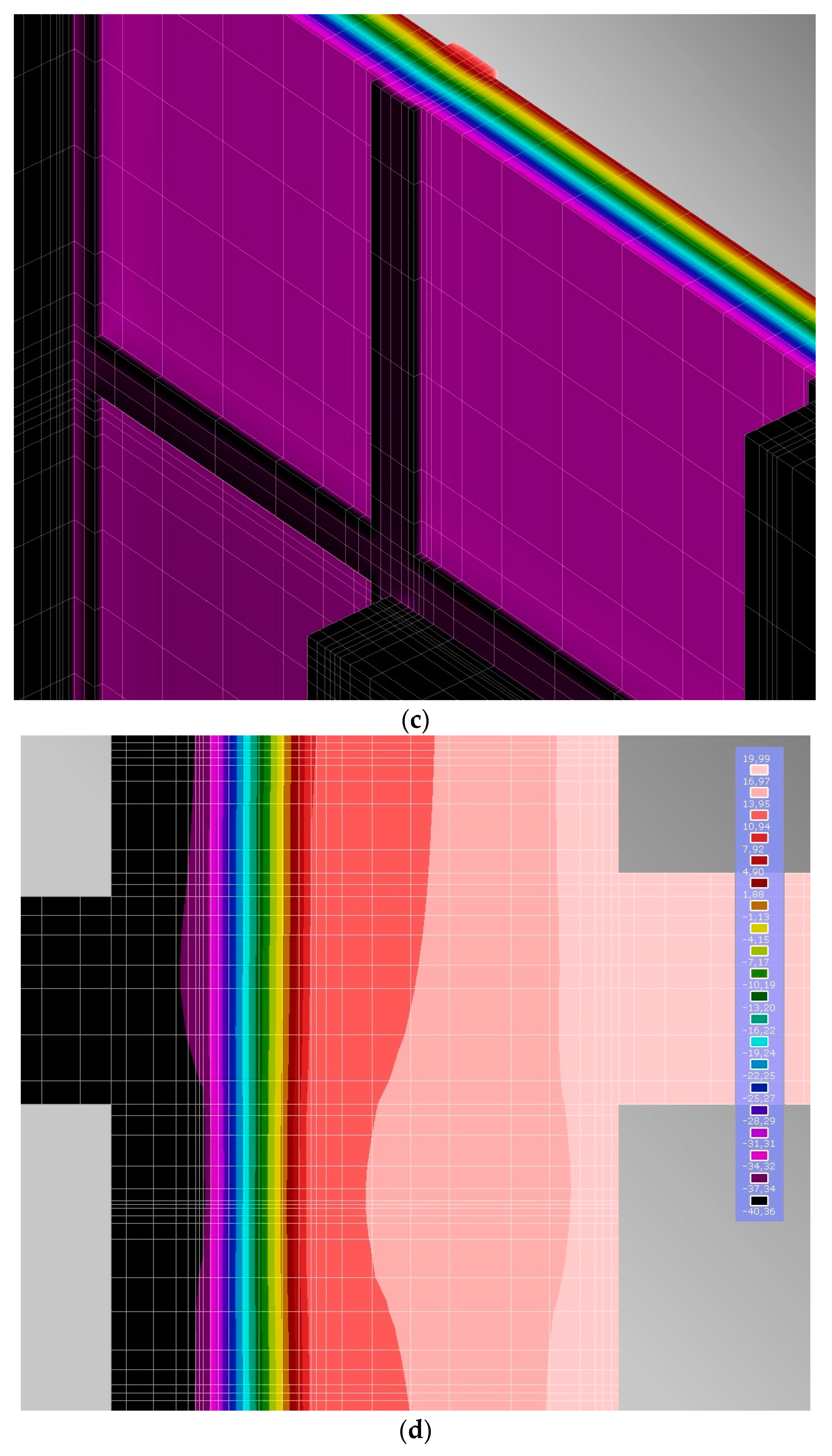
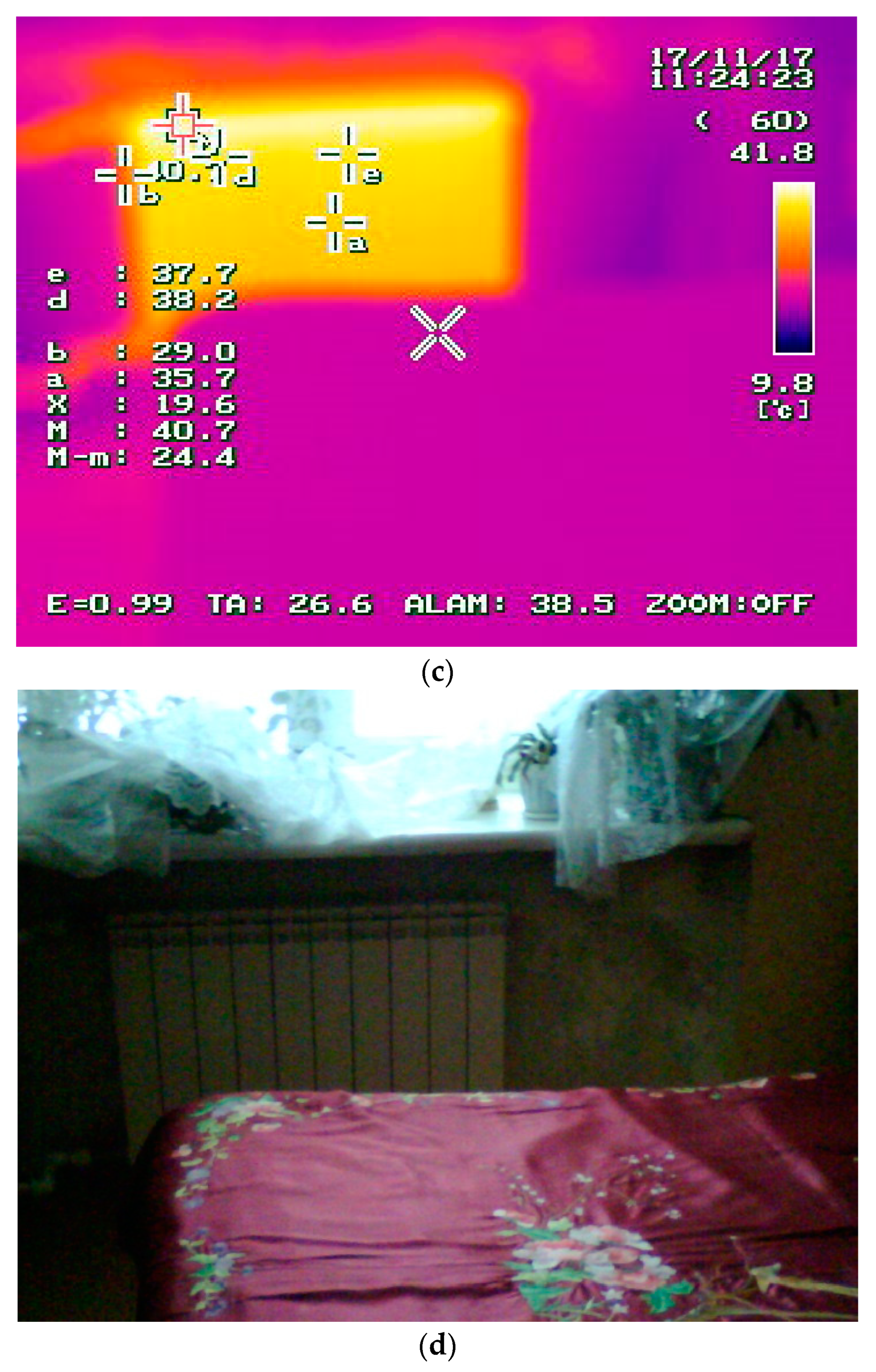
Figure 1 indicates the temperature profiles of window and balcony doors resulting in additional heat consumption during the coldest period of the year.
For the same boundary conditions and the same structural construction, Figure 1 shows the distribution of indoor temperature according to the novel methodology that also includes an increased heat demand compared to the reference scenario. Around 10% of heat (excessive amount of energy above the design threshold) is lost according to this calculation. In the case of an old building used for commercial purposes, it is covered by an even higher heat demand increase (up to 20%) between 7 a.m. and 5 p.m. Otherwise, the drop in indoor temperature is expected at 17:00, which corresponds to the reduction in internal heat gains in office buildings and the same energy consumption at that time. Secondly, the approach based on adjusted variables (Rinf.door and k) was only able to indicate the variation of temperature fields closer to the thermography. Temper software also adapts to the change in indoor temperature requirements, maintaining more accurate boundary conditions within the zone, despite any learning that goes on during static deployment. For instance, Figure 1d shows the surface temperature of 19.9 °C rather than 4.9 °C in Figure 1c.
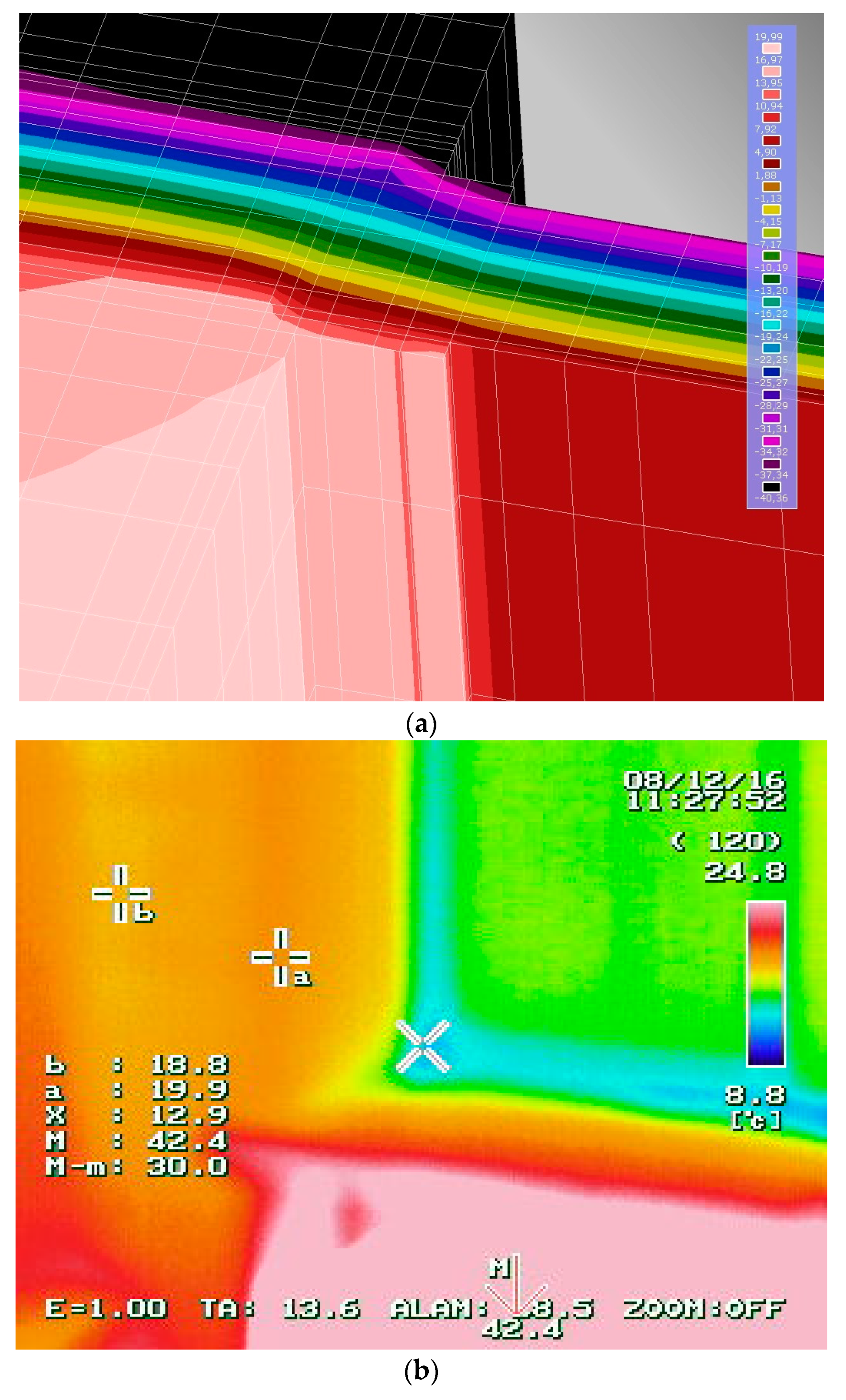
The next step of the methodology is to study the edges of the wall and ceiling with different temperatures, as displayed in Figure 2.
To enhance the thermal performance of worn-out structures and consequently decrease energy consumption, the integration of the actual temperature distribution of inner surface wallboards or furniture elements is a promising decision. In the present research, taking the contents of the apartment into account may increase the U-factor by 1.56 and 1.17 times in the cases of low-insulation and high-insulation light-structure houses, respectively.
As mentioned above, the performance of the envelopes is the key factor defining the heat demand of a building. When R is fixed at 3.15 or 0.54 m2 °C/W with β set to 0.1 or 0.05, the effected heat consumption is up to 444 W, which is purely according to the characteristics described in Figure 2. The average error is found then to be in the range of 5%, with some values above, indicating that the suggested methodology is more correct when assessing heat demand. In response to the increasing factors of insolation and internal heat gains to 51 W/m3 and 68 W/m3, respectively, the prediction errors for the linear temperature model increase. Correcting a traditional approach when designing a building may minimize the peak energy consumption by 23.3% and increase the annual performance by up to 14.1%.
To compare, Ren et al. [27] assume a specific heat transfer of 34 W/m3 with a U-value below 0.063; the maximum error is then 20%, which is much lower compared to those presented here. This results in a 5% or less discrepancy, indicating that their model has a low error when forecasting indoor temperature. According to Johra et al. [29], furniture with advanced analysis could increase the heat demand by up to 87 and 30% in the cases of low-insulation and high-insulation light-structure houses, respectively. Ren et al. [27] conclude when setting heat transfer to 51 and 68 W/m3, the prediction errors for a linear model increase.
Table 1 indicates that the heat demand is much lower before adopting factors for thermal inertia, and the variation is also large for different offices, with a total difference of 6952.6 and an average of 54.7 W.
When assessing a big mall, an office building, or an ice-skating rink with multiple doors, the difference is expected to be much larger. After adopting the suggested methodology, the standard deviation is 1404.1 W, the variation amplitude for each space is small, with a maximum value of 2.072, a minimum value of 1.05, and an average of 1.07. Thus, compared with the traditional approach, the new one may ensure better indoor comfort. At the same time, it decreases energy consumption for the operation of the DH network. Currently, the heat demands of the closest rooms to the windows oriented to the south do not result in 26 °C, while the heat demands of the other spaces are still mostly affected by the internal heat gains due to the consumers’ behavior (previously obtained when the consumption was still detected).
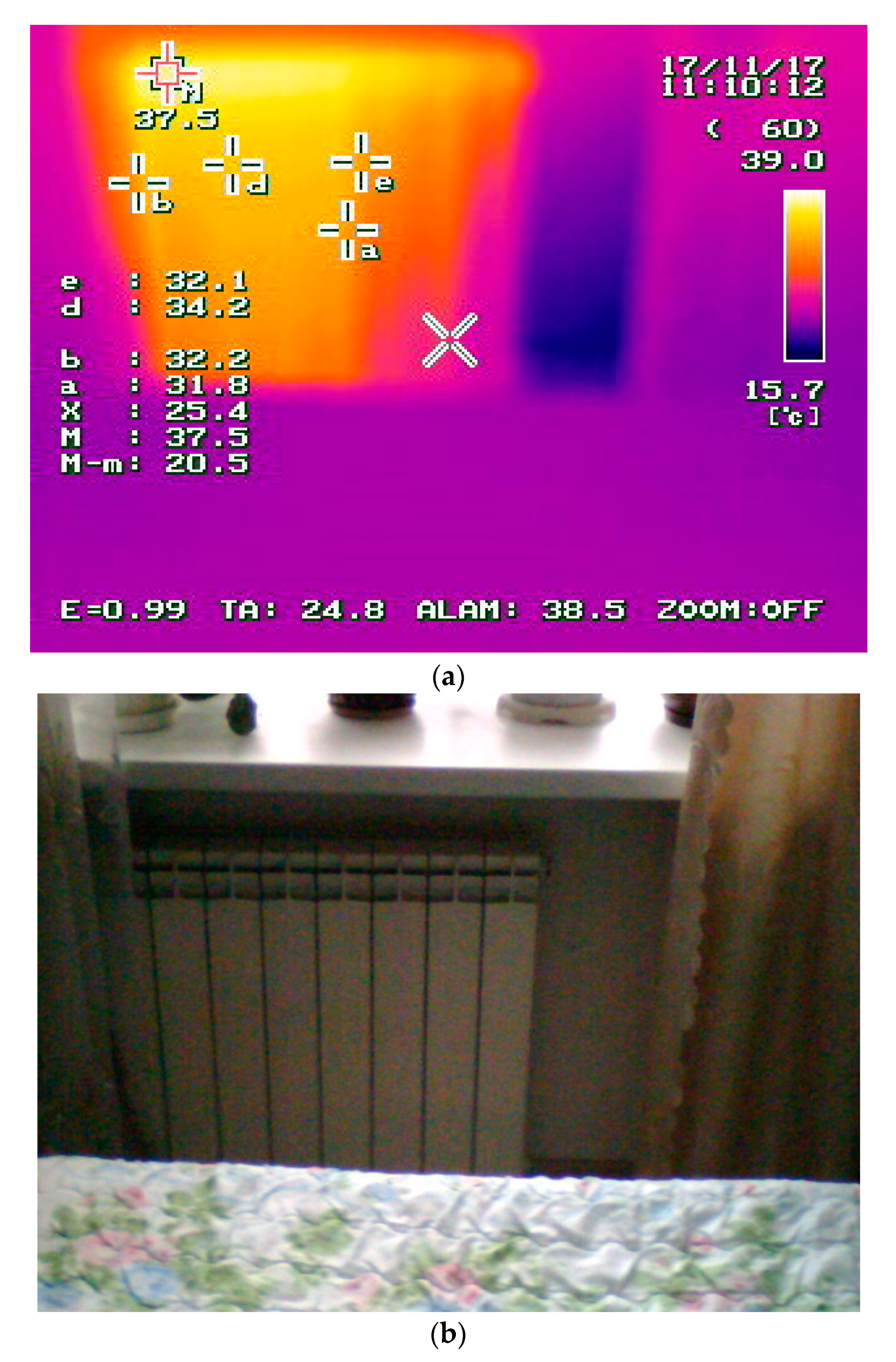
Therefore, an additional study at a residential building has been performed to quantify the contribution of the faulty components of a SH system or additional heaters in the creation of the peaks of return temperature; the results are shown in Figure 3.
This results in lowering the temperature difference between the supply and return lines, which is an average of 16.5 °C. Hence, a larger amount of hot water inflows, although less heat per radiator is absorbed, much lower than regulated by the DH design guidelines to ensure 25 °C. This keeps the secondary return temperature high, consequently increasing the return temperature for a DH plant receiving return water from such a substation. This trend has been recorded in 31% of the inspected buildings. This results in the overheating of some spaces, the lowering of the indoor temperature (from the design one) in others, and also goes hand in hand with poor hydronic balancing being either a reason or a consequence. Even once a SH system is perfectly balanced, the return temperature after the substation may be still higher by 10–15%, and to address this issue, modernizing a substation is required. This could be also reasoned by consumers who install additional radiators to their SH systems to ensure comfort considerations. The issues reported by Kristensen et al. [4], such as ensuring warm feet on tiled bathroom floors by ordinary SH systems instead of maintaining the overall indoor temperature, are difficult to encounter in Russian cities such as Omsk or Krasnoyarsk.
To compare, Jangsten et al. [24] detected a trend of running at higher return temperature with an error of more than 1–2 °C, which is prescribed by the district cooling design guidelines. This behavior has been detected in 59% of the inspected buildings. The same was detected by Luc et al. [25], with the influence of internal heat gains also being visible for both new and old commercial buildings, where the temperature starts to increase after beginning a working day when the internal heat gains intensify. When looking at the graphs with the daily resolution, the same trend can be justified by considering the shortages of heat delivery due to the supply temperature being limited to 118 °C instead of the design upper threshold of 150 °C [30]. During these periods, the deviations are the largest ones (about 10–20 °C), while there is a threshold of outdoor temperature when the correct profile is achieved (about −15 °C). Thus, at −15 °C and above, no additional energy consumption is recorded. Once again, compared with Luc et al. [25], the increase in indoor temperature is caused by consumer’s changes in the SH system such as changing radiators, installing or demounting electronic devices, and heat gains coming from electric heaters rather than from electronic device use and from occupants.

4. Conclusions

Newer buildings have a lower but smoother profile of indoor temperature, whereas in older buildings, the indoor temperature might be unreasonably high, being 25–30 °C. The methodology suggests correction factors to enable a more thorough technical and economic review of a DH system. A better understanding of the system operation constitutes a necessary step in the process of switching to the 4GDH. An ordinary design approach results in the maximum possible demand of 299.7 kW. We suggest dumping heat with an indoor temperature of 20–25 °C by using the storage capacity of building envelopes, with no peak units (e.g., a heat pump) at all. Correcting a traditional approach when designing a building may minimize the energy consumption to 262.9 kW and increase the annual performance by up to 14.1%. The expected operation of both optimal designs (with the condition of optimal management of the substation) was analyzed with the help of the thermograms and modeling software. This means that the substation is assumed to be managed perfectly in line with design conditions, with no faulty equipment or any other operational issues such as increasing return temperature.
As suggested by the literature review, all the data-driven approaches agree on further tightening regulations of energy performance and a step-by-step conversion to 4GDH. Eventually, huge advantages may be achieved by the modernization of a conventional controller at a DH substation before two other primary steps (installing TES and running in low-temperature mode). The reductions in the thermal peak resulting from a new type of controller adjustment (for instance, discrete) compared to the traditional operation range from roughly 10 to 30%, respectively. This methodology simplifies all the implementations, accelerating the transition of district energy systems to new generations.

Author Contributions

Conceptualization, S.C. and A.Z.; methodology, S.C.; software, S.C.; validation, S.C., A.Z., and L.J.; formal analysis, S.C.; investigation, S.C.; resources, S.C.; data curation, S.C.; writing—original draft preparation, S.C.; writing—review and editing, S.C. and A.Z.; visualization, S.C.; supervision, A.Z.; project administration, A.Z.; funding acquisition, A.Z. All authors have read and agreed to the published version of the manuscript.

Funding

This research received no external funding.

Institutional Review Board Statement

Not applicable.

Informed Consent Statement

Not applicable.

Data Availability Statement

The data presented in this study are available on request from the corresponding author. The data is not publicly available due to confidentiality reasons.

Conflicts of Interest

The authors declare no conflict of interest.

References

  1. Fitó, J.; Hodencq, S.; Ramousse, J.; Wurtz, F.; Stutz, B.; Debray, F.; Vincent, B. Energy- and exergy-based optimal designs of a low-temperature industrial waste heat recovery system in district heating. Energy Convers. Manag. 2020, 211, 112753. [Google Scholar] [CrossRef]
  2. Guelpa, E. Impact of thermal masses on the peak load in district heating systems. Energy 2021, 214, 118849. [Google Scholar] [CrossRef]
  3. Turski, M.; Sekret, R. Buildings and a district heating network as thermal energy storages in the district heating system. Energy Build. 2018, 179, 49–56. [Google Scholar] [CrossRef]
  4. Kristensen, M.H.; Hedegaard, R.E.; Petersen, S. Long-term forecasting of hourly district heating loads in urban areas using hierarchical archetype modeling. Energy 2020, 201, 117687. [Google Scholar] [CrossRef]
  5. Brandi, S.; Piscitelli, M.S.; Martellacci, M.; Capozzoli, A. Deep reinforcement learning to optimise indoor temperature control and heating energy consumption in buildings. Energy Build. 2020, 224, 110225. [Google Scholar] [CrossRef]
  6. Aryal, A.; Chaiwiwatworakul, P.; Chirarattananon, S. An experimental study of thermal performance of the radiant ceiling cooling in office building in Thailand. Energy Build. 2023, 283, 112849. [Google Scholar] [CrossRef]
  7. Vandermeulen, A.; van Oevelen, T.; van der Heijde, B.; Helsen, L. A simulation-based evaluation of substation models for network flexibility characterisation in district heating networks. Energy 2020, 201, 117650. [Google Scholar] [CrossRef]
  8. Sun, C.; Chen, J.; Cao, S.; Gao, X.; Xia, G.; Qi, C.; Wu, X. A dynamic control strategy of district heating substations based on online prediction and indoor temperature feedback. Energy 2021, 235, 121228. [Google Scholar] [CrossRef]
  9. Yuan, J.; Huang, K.; Han, Z.; Zhou, Z.; Lu, S. A new feedback predictive model for improving the operation efficiency of heating station based on indoor temperature. Energy 2021, 222, 119961. [Google Scholar] [CrossRef]
  10. Sleptsov, A.; Crisostomi, E.; Bischi, A. Control schemes for district heating substations considering user-defined building’s indoor temperature. Build. Environ. 2021, 191, 107598. [Google Scholar] [CrossRef]
  11. Ivanko, D.; Sørensen, Å.L.; Nord, N. Splitting measurements of the total heat demand in a hotel into domestic hot water and space heating heat use. Energy 2021, 219, 119685. [Google Scholar] [CrossRef]
  12. Chicherin, S.; Zhuikov, A.; Junussova, L. Integrating a heat pump into a 4th generation district heating (4GDH) system—Two-mode configuration inputting operational data. Energy Build. 2022, 275, 112445. [Google Scholar] [CrossRef]
  13. Saletti, C.; Zimmerman, N.; Morini, M.; Kyprianidis, K.; Gambarotta, A. Enabling smart control by optimally managing the State of Charge of district heating networks. Appl. Energy 2020, 283, 116286. [Google Scholar] [CrossRef]
  14. Braas, H.; Jordan, U.; Best, I.; Orozaliev, J.; Vajen, K. District heating load profiles for domestic hot water preparation with realistic simultaneity using DHWcalc and TRNSYS. Energy 2020, 201, 117552. [Google Scholar] [CrossRef]
  15. Aste, N.; Caputo, P.; Del Pero, C.; Ferla, G.; Huerto-Cardenas, H.E.; Leonforte, F.; Miglioli, A. A renewable energy scenario for a new low carbon settlement in northern Italy: Biomass district heating coupled with heat pump and solar photovoltaic system. Energy 2020, 206, 118091. [Google Scholar] [CrossRef]
  16. Sommer, T.; Sulzer, M.; Wetter, M.; Sotnikov, A.; Mennel, S.; Stettler, C. The reservoir network: A new network topology for district heating and cooling. Energy 2020, 199, 117418. [Google Scholar] [CrossRef]
  17. Kauko, H.; Kvalsvik, K.H.; Rohde, D.; Nord, N.; Utne, Å. Dynamic modeling of local district heating grids with prosumers: A case study for Norway. Energy 2018, 151, 261–271. [Google Scholar] [CrossRef]
  18. Hering, D.; Cansev, M.E.; Tamassia, E.; Xhonneux, A.; Müller, D. Temperature control of a low-temperature district heating network with Model Predictive Control and Mixed-Integer Quadratically Constrained Programming. Energy 2021, 224, 120140. [Google Scholar] [CrossRef]
  19. Brange, L.; Englund, J.; Lauenburg, P. Prosumers in district heating networks—A Swedish case study. Appl. Energy 2016, 164, 492–500. [Google Scholar] [CrossRef]
  20. Chertkov, M.; Novitsky, N.N. Thermal Transients in District Heating Systems. Energy 2019, 184, 22–33. [Google Scholar] [CrossRef]
  21. Farouq, S.; Byttner, S.; Bouguelia, M.-R.; Nord, N.; Gadd, H. Large-scale monitoring of operationally diverse district heating substations: A reference-group based approach. Eng. Appl. Artif. Intell. 2020, 90, 103492. [Google Scholar] [CrossRef]
  22. Chicherin, S.; Starikov, A.; Zhuikov, A. Justifying network reconstruction when switching to low temperature district heating. Energy 2022, 248, 123618. [Google Scholar] [CrossRef]
  23. Siuta-Olcha, A.; Cholewa, T.; Gomółka, M.; Kołodziej, P.; Østergaard, D.S.; Svendsen, S. On the influence of decommissioning an area thermal substation in a district heating system on heat consumption and costs in buildings—Long term field research. Sustain. Energy Technol. Assess. 2022, 50, 101870. [Google Scholar] [CrossRef]
  24. Jangsten, M.; Lindholm, T.; Dalenbäck, J.O. Analysis of operational data from a district cooling system and its connected buildings. Energy 2020, 203, 117844. [Google Scholar] [CrossRef]
  25. Luc, K.M.; Li, R.; Xu, L.; Nielsen, T.R.; Hensen, J.L.M. Energy flexibility potential of a small district connected to a district heating system. Energy Build. 2020, 225, 110074. [Google Scholar] [CrossRef]
  26. Harney, P.; Gartland, D.; Murphy, F. Determining the optimum low-temperature district heating network design for a secondary network supplying a low-energy-use apartment block in Ireland. Energy 2020, 192, 116595. [Google Scholar] [CrossRef]
  27. Ren, C.; Cao, S.J. Construction of linear temperature model using non-dimensional heat exchange ratio: Towards fast prediction of indoor temperature and heating, ventilation and air conditioning systems control. Energy Build. 2021, 251, 111351. [Google Scholar] [CrossRef]
  28. Camci, M.; Karakoyun, Y.; Acikgoz, O.; Dalkilic, A.S. A comparative study on convective heat transfer in indoor applications. Energy Build. 2021, 242, 110985. [Google Scholar] [CrossRef]
  29. Johra, H.; Heiselberg, P.; Le Dréau, J. Influence of envelope, structural thermal mass and indoor content on the building heating energy flexibility. Energy Build. 2019, 183, 325–339. [Google Scholar] [CrossRef]
  30. Chicherin, S.; Anvari-Moghaddam, A. Adjusting Heat Demands Using the Operational Data of District Heating Systems. Energy 2021, 235, 121368. [Google Scholar] [CrossRef]
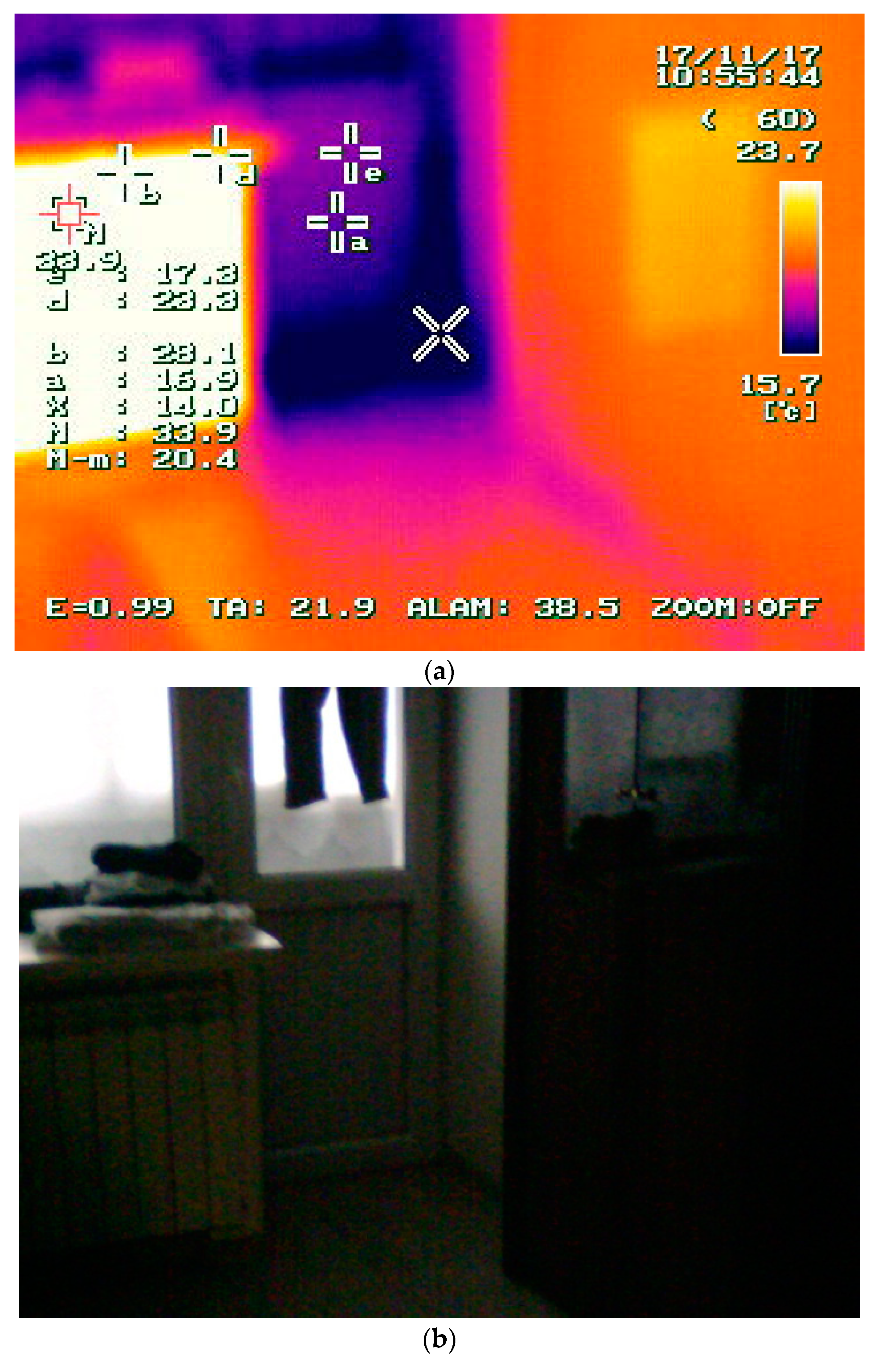
Figure 1. Temperature profiles and visual imagery: (a,b) actual, (c) modeled as traditional. The temperature profiles are even and smooth and all the borders between temperature zones are represented by straight lines; (d) simulated setting of actual temperatures as boundary conditions and applying β-factor for a door.
Sustainability 15 14908 g001aSustainability 15 14908 g001b
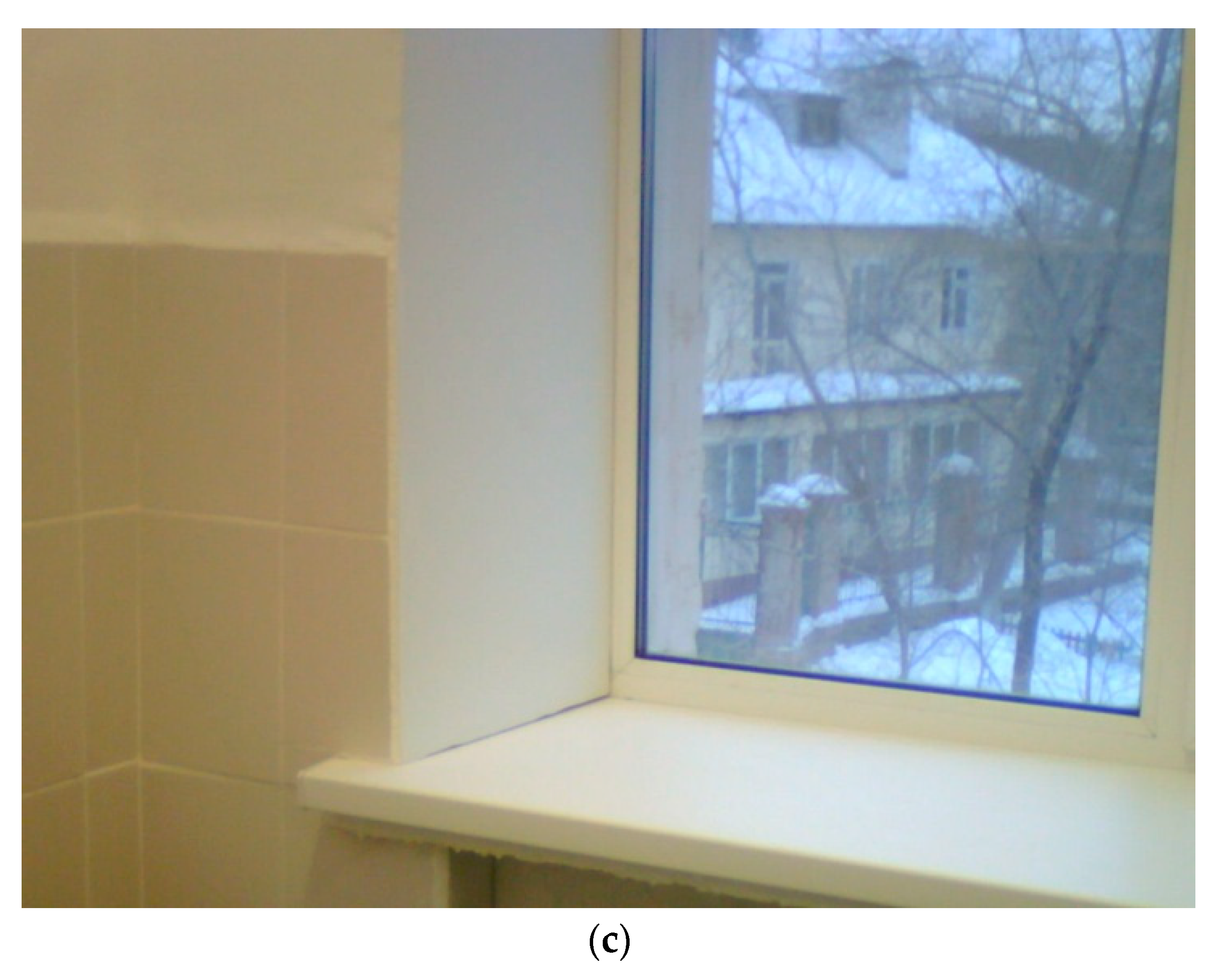
Figure 2. Contours of temperature (a) compared to actual temperatures (b) obtained from the Temper-3d© simulation and linear temperature model applied to a typical window (c).
Sustainability 15 14908 g002aSustainability 15 14908 g002b
Figure 3. A radiator of a SH system: (a,b), an old one, which is not even hot; (c,d), the same conditions and the same location but another room where a new radiator was installed. Note that although the maximum temperature is only 2.8 °C higher, it is the same for the whole radiator surface.
Sustainability 15 14908 g003aSustainability 15 14908 g003b
Table 1. The adjustment factors and heat consumption corresponding to different zones. There is one main entrance and several emergency exits on the ground- and first floors, in addition to fire escapes on the second, third, and fourth floors. Walls adjacent to the indoor spaces with colder design indoor temperature (e.g., a staircase or a vestibule) contributing to overall heat losses are titled ‘internal partitions’.
#Office (Zone)Target Indoor Temperature [°C]Properties of EnvelopesR-Value [m2K/W]tindtoutdDesign Heat Demand [W]CorrectionsAdjusted Heat Demand [W]Total Heat Demand [W]
Wall Title (According to the Blueprints)OrientationAdjustment Factor βAdjustment Factor kOverall Correction (1 + Σβ)
1Tool shop16Internal partition #1 2.15328620n/a1.028626325
16Internal partition #2 4.35313610n/a1.01361
16Internal partition #3 8.6537240n/a1.0724
16Internal partition #4 14.2536760n/a1.0676
16WindowNE0.54534240.10.81.1466.6
16DoorSW0.5453235011.0235
2Storage room for household chemical goods. garage16Internal partition #1 2.15334080n/a1.034087835
16Internal partition #2 4.35319350n/a1.01935
16Internal partition #3 8.6538760n/a1.0876
16Internal partition #4 14.2538140n/a1.0814
16WindowNE0.54534940.10.81.1544
16DoorNW0.54532350.111.1258
13Office20Load-bearing wallSW3.15572350n/a1.0235708
20Load-bearing wallNW3.15574300.1n/a1.1473
12Exhibition hall20Load-bearing wallSW3.15578600n/a1.08608569
20WindowSW0.5457912−0.10.80.9821
20Load-bearing wallSE3.1557664−0.05n/a0.95632
20WindowSE0.54571158−0.050.80.951103
20Load-bearing wallNW3.15577040.1n/a1.1774
20DoorNE0.54574560.111.1502
20Load-bearing wallNE3.15575210.1n/a1.1573
20WindowNE0.54573360.10.81.1370
20Load-bearing wallNE3.15573910.1n/a1.1430
20DoorNW0.54574560.111.1502
20WindowSW0.5457912−0.10.80.9821
Staircase/
Vestibule
16Load-bearing wallSW3.1553182−0.1n/a0.91641102
16Load-bearing wallNW3.15534480.1n/a1.1493
16Load-bearing wallNE3.15531820.1 + 0.27 × 3.6n/a2.072377
16DoorNE0.54532060.111.1227
2Vestibule20Load-bearing wallSW3.15572780n/a1.0278936
20DoorSW0.5457329−0.110.9296
3Office20WindowNE0.545719000.10.81.120904720
20WindowSE0.54571900−0.050.80.951805
20Internal partition #1 2.1575430n/a1.0543
20Internal partition #2 4.357900n/a1.090
20Internal partition #3 8.65720n/a1.02
Staircase16Load-bearing wallNW3.15574180.1n/a1.14601334
16Load-bearing wallNE3.15573000.1n/a1.1330
16Load-bearing wallSW3.15573000n/a1.0300
16DoorNW0.54572220.111.1244
4Exhibition hall20Load-bearing wallNW3.15573910.1n/a1.143017,294
20Load-bearing wallSW3.15575210n/a1.0521
20WindowSW0.545789700.81.0897
20WindowSE0.545776000.050.81.057980
20Load-bearing wallNE3.155713680.1n/a1.11505
20DoorNE0.54573290.111.1362
20WindowNE0.545713680.10.81.11505
20Load-bearing wallNW3.15577820.1n/a1.1860
20WindowNW0.54576840.10.81.1752
20DoorNW0.54574560.111.1502
20Internal partition #1 2.15713570n/a1.01357
20Internal partition #2 4.3575040n/a1.0504
20Internal partition #3 8.6571190n/a1.0119
12Office20WindowSW0.5457831200.81.0831216,822
20WindowNW0.545739580.10.81.14354
20WindowSE0.545739580.050.81.054156
Staircase16Load-bearing wallNE3.15533790.1n/a1.14171955
16WindowNE0.54533680.10.81.1405
16Load-bearing wallSW3.15535610.05n/a1.05589
16Load-bearing wallNW3.15531260.1n/a1.1139
16WindowNW0.54533680.10.81.1405
6Hallway20Load-bearing wallNW3.15574260.1n/a1.14692001
20DoorNW0.54572590.111.1285
20Load-bearing wallNW3.15571220.1n/a1.1134
20Load-bearing wallNE3.15572770.1n/a1.1305
20WindowNE0.54572850.10.81.1314
20Load-bearing wallSE3.15571440.05n/a1.05151
20WindowNW0.54571900.10.81.1209
11Office20WindowSW0.5457237500.81.023752375
19Office20Load-bearing wallNE3.15572710.1n/a1.12981164
20WindowNE0.54571900.10.81.1209
20Load-bearing wallNW3.15574070.1n/a1.1448
20WindowNW0.54571900.10.81.1209
1Office20Load-bearing wallNW3.15574070.1n/a1.1448657
20WindowNW0.54571900.10.81.1209
2.3Office20Load-bearing wallNE3.15578140.1n/a1.18951731
20WindowNE0.54577600.10.81.1836
4Office20Load-bearing wallNE3.15573390.1n/a1.13732224
20Load-bearing wallNE3.15576110.1n/a1.1672
20Load-bearing wallSE3.15574070.05n/a1.05427
20WindowNE0.54576840.10.81.1752
5Office20WindowSE0.545723750.050.81.0524942494
10Office20WindowSE0.545747500.050.81.0549888155
20WindowSW0.5457316700.81.03167
14Office20Load-bearing wallNW3.15574070.1n/a1.1448646
20WindowNW0.54571800.10.81.1198
20Office20Load-bearing wallNW3.15574070.1n/a1.14483976
20Load-bearing wallSW3.15572040n/a1.0204
20WindowNW0.545715830.10.81.11741
20WindowSW0.5457158300.81.01583
14Office20WindowNW0.545731320.10.81.1344512,754
20WindowSW0.5457313200.81.03132
20WindowSE0.545735690.050.81.053748
20WindowNE0.545718210.10.81.12003
20Internal partition 4.18574260n/a1.0426
5Office20WindowNE0.545724040.10.81.126446341
20WindowNW0.545732050.10.81.13526
20DoorNW0.54571550.111.1171
1Security room20WindowNW0.54578740.10.81.1961961
13Hallway20WindowNW0.54579470.10.81.110421376
20DoorSE0.54572220.0511.05233
20WindowSW0.545710100.81.0101
9Lounge20WindowSE0.545733500.050.81.0535184975
20WindowSW0.5457145700.81.01457
6Exhibition hall20WindowNE0.545744430.10.81.148876990
20WindowSE0.545720030.050.81.052103
Vestibule20WindowSW0.5457218500.81.021852185
7Vestibule18WindowSE0.545542200.81.0422422
3Vestibule18WindowNW0.54553510.10.81.1386386
15Vestibule18WindowSW0.545535100.81.0351351
2Principal’s office20WindowSW0.5457171000.81.017104569
20Internal partition 4.18572460n/a1.0246
20WindowNW0.545723750.10.81.12613
1Reception20Internal partition 4.18572460n/a1.02464565
20WindowNE0.545717860.10.81.11965
20WindowЮB0.545722420.050.81.052354
4Bathroom20WindowNE0.54574560.10.81.1502502
3Lounge area20WindowNE0.545714250.10.81.115682509
20WindowNW0.54578550.10.81.1941
Disclaimer/Publisher’s Note: The statements, opinions and data contained in all publications are solely those of the individual author(s) and contributor(s) and not of MDPI and/or the editor(s). MDPI and/or the editor(s) disclaim responsibility for any injury to people or property resulting from any ideas, methods, instructions or products referred to in the content.