Analyzing the Drivers of Agricultural Irrigation Water Demand in Water-Scarce Areas: A Comparative Study of Two Regions with Different Levels of Irrigated Agricultural Development

Abstract

Both the demand for agricultural irrigation and the level of water-saving technology in water-scarce regions have met food demand with technological progress and economic growth. There are differences in irrigation water demand drivers in regions with different levels of irrigated agricultural development. However, the relationship between related drivers in response to regional irrigation water demand is not fully understood. This study quantified the driving influence of six indicators, including technological progress, planting structure, water conservation management, economic development, planting scale, and consumption intensity, on agricultural irrigation water demand in JC (Jinchang) and WW (Wuwei), two cities in the Shiyang River Basin, from 2011 to 2020. The results shows that economic development is the main driver of the increase in irrigation water demand, with 29% and 43% driving contributions in JC and WW, respectively. Consumption intensity contributes the most to the decrease in irrigation water demand, with 31% and 23% of driving contribution in JC and WW, respectively. Cropping size has a greater positive drive on irrigation water demand in non-agricultural areas relative to agricultural areas. Planting structure has a more pronounced negative drive on irrigation water demand in agricultural areas relative to non-agricultural areas. In particular, relative to irrigated areas, the proportion of water-saving irrigated areas to the sown areas has a greater impact on changes in irrigation water demand, with a significant rebound effect when it exceeds 80%, so that blindly expanding water-saving irrigated areas will drive an increase in irrigation water demand. The results of this study can provide useful suggestions for agricultural water management in water-scarce areas with different levels of water-saving irrigation development, and realize the sustainable development of agriculture in water-scarce areas.

1. Introduction

Water management for agricultural irrigation is important for water-scarce areas. Irrigation water demand is affected by a combination of natural and artificial systems. Natural system influences include climate change [1], soil environment [2], etc. According to the studies conducted by Shikun [3] and Yetong Li [4], it has been concluded that irrigation water demand is less influenced by climate change and more influenced by anthropogenic factors, accounting for over 80% of the variability. Artificial systems, such as planting scale, planting structure [5], irrigation methods [6], agricultural productivity [7], and socioeconomics [8] factors, have a direct or indirect impact on irrigation water demand. For instance, the adoption of water-saving irrigation techniques can enhance the efficiency of water utilization and consequently reduce irrigation water demand [9]. However, it may also lead to changes in planting structure and scale [10], and even result in a rebound effect [11]. Indirectly, socio-economic factors, including the level of economic development and urbanization [12], influence irrigation water demand through their impact on agricultural production and technological development [13,14]. In water-scarce areas, agricultural production faces additional water stress [15], necessitating limited water resources to produce substantial amounts of food [16]. Furthermore, water resources act as a constraint on crop production and economic growth [17,18]. Quantifying the impacts of irrigation water demand drivers in water-scarce areas can improve the adaptability of regional irrigated agriculture, which is important for irrigation and agricultural production in water-scarce areas.

The quantitative assessment of the factors influencing irrigation water demand is complex. In the stage of conducting analysis on the drivers of irrigation water demand, the logarithmic mean Divisia index method (LMDI) is highly applicable and commonly used in agricultural irrigation water analysis [19,20]. Agricultural management indicators, including planting scale, planting structure, and technology level, are frequently utilized as drivers in assessing agricultural irrigation water demand [21,22,23]. Zou et al. considered planting scale, planting pattern, climate change, and water-saving technology in the LMDI decomposition analysis of irrigation water demand in arid basins [9]. Liu considered water conservation management factors in the analysis of agricultural water-use drivers [24]. Zhao et al. showed that economic effect is the largest positive contributor to the in-crease in the agricultural water footprint [20]. Zeng et al. found that economic level is the largest contributor to the growth of irrigation water demand, and water use intensity is the most important factor inhibiting the growth of irrigation water demand [25].Hence, it is crucial to comprehensively consider both agricultural management and socio-economic factors when quantitatively analyzing the relationship between these drivers and irrigation water demand. Doing so can provide valuable insights to guide the development of agricultural production and irrigation plans in regions that experience water scarcity. In addition, it is worth noting that existing studies have primarily focused on regional or inter-basin analyses, lacking inter-regional comparative analysis. This knowledge gap hinders a thorough understanding of the response relationship between irrigation water demand and its drivers.

This paper focuses on JC and WW, situated within the Shiyang River Basin in Gansu Province. This study aims to achieve the following objectives: (i) assess the irrigation water demand in JC and WW from 2011 to 2020; and (ii) establish a model to analyze the driving factors of irrigation water demand, quantifying the influences of six factors: technological progress, planting structure, water-saving management, economic development, planting scale, and consumption intensity, on irrigation water demand. This study aims to uncover the driving forces behind irrigation water demand in water-scarce areas at various levels of irrigation development. The findings will furnish researchers and policy-makers with valuable insights for agricultural production and water resource management in water-scarce areas.

2. Materials and Methods

2.1. Study Area

The study area of this research is Jinchang City (JC) and Wuwei City (WW), including both urban and rural areas within these two regions. JC and WW are located in Gansu Province, China (Figure 1), and the two cities belong to the same major administrative region of the Shiyang River Basin, with more than 60% of their water supply sources supplying water. The average annual precipitation of JC for the period of 2011–2020 was 212 mm, and that of WW was 231 mm. JC and WW belong to the same temperate continental arid climate; the region is dry, with little rain, and precipitation distribution is not uniform.

According to the statistical analysis of the Gansu Province Water Resources Bulletin, the average annual per capita self-produced water resources in JC was 184 m³/person from 2013 to 2020, and the average annual per capita self-produced water resources in WW was 678 m³/person. The average annual per capita water consumption in JC is 1489 m³/person, and the water consumption per unit of GDP decreases from 289 m³/10⁴ RMB to 184 m³/10⁴ RMB, while the average per capita water consumption in WW is 871 m³/person, and the water consumption per unit of GDP decreases from 412 m³/10⁴ RMB to 312 m³/10⁴ RMB. The analysis of the water resource statistics of JC and WW found that JC is more scarce in water resources relative to WW, but the per capita water intensity is higher than that of WW, and the efficiency of water use is higher than that of WW.

The development of irrigated agriculture in JC and WW is not the same due to differences in water resource endowment. From 2011 to 2020, the share of cultivated land areas in JC increased from 1.34% to 2.21%, while the share in WW rose from 7.61% to 13.82%. The ratio of effective irrigated farmland areas to cultivated land areas in JC is relatively stable and above 80%, while the effective irrigated farmland areas in WW shows an increasing trend, but with the growth in cultivated land area, its ratio shows a decreasing trend, and the ratio was less than 50% in 2018–2020. The proportion of water-saving irrigation to sown areas is larger in JC than in WW. Although WW has a more developed planting industry compared to JC, the level of water-saving technology is higher in JC.

2.2. Data Description

The period from 2011 to 2020 is used for the decomposition analysis in this study, including the two cities of JC and WW, in which six major crops of wheat, corn, yams, oilseeds, vegetables, and fruiters are represented. This study is divided into the calculation of irrigation water demand and a decomposition analysis of irrigation water demand.

Irrigation water demand is calculated based on the following factors: the net irrigation quota, crop sown area, and irrigation water utilization coefficient. The product of the net irrigation quota and the sown areas of the crop is compared to the irrigation water utilization coefficient to obtain the actual irrigation water requirement of the area. The net irrigation quota is the amount of irrigation water utilized by the crop per unit of irrigated areas during the crop’s reproductive period, and is calculated using meteorological data and crop fertility data. The meteorological data include the day-by-day air temperature, wind speed, relative humidity, sunshine hours, and precipitation from 23 weather stations in Gansu Province during 2011–2020, and were obtained from the National Meteorological Science Data Center (http://www.nmic.cn/, accessed on 12 July 2022). The crop fertility data include crop coefficients for the fertility period. The crop coefficients reflect the difference in water requirements between the crop and the reference crop, and are largely dependent on the growth and development of the crop canopy. The FAO divides crop fertility into four stages: early, developing, middle, and late. The crop fertility stages and crop coefficients used in this study were obtained from the research results of Zhang Hua [26,27], Tong Ling [28], and the FAO crop database, with appropriate adjustments. The crop sown areas were obtained from the Gansu Provincial Statistical Yearbook 2011–2021. The irrigation water utilization coefficient (IWUC) is the ratio of the effective amount of water actually irrigated into the farmland that can be absorbed and utilized by the crop to the amount of water introduced into the head of the canal, representing the efficiency of the crop in using irrigation water. In this study, the irrigation water utilization coefficient of Gansu Province is used to represent the irrigation water utilization coefficient of the two regions. The data were obtained from the research results of Gu He [29] and the China Water Resources Bulletin (2011–2020).

Irrigation water demand can be decomposed into the following factors for calculation: technological development, cropping structure, the scale of cultivation, water-saving management, economic development, and consumption intensity. Technological development is the ratio of crop irrigation water demand and crop yield, which represents crop water-use efficiency and is closely related to the level of technology. Cropping structure is a question of the proportion of crop types grown in a region or country, and in this study the crop yield percentage studies the cropping structure. The irrigated crop water demand is derived from the above calculations, and the crop production information is derived from the Gansu Provincial Statistical Yearbook 2012–2021. The planting scale is the total sown area of various crops. Water-saving irrigation is the irrigation measure to obtain maximum yield or income with minimum water consumption, that is, to maximize crop yield and output value per unit of irrigation water, including sprinkler and drip irrigation, micro-irrigation, low-pressure pipe irrigation, channel seepage control, and other water-saving measures. The area of water-saving irrigation includes the area of the above water-saving measures, and the data are from the Gansu Water Resources Bulletin 2011–2020. Economic development is the ratio of the agricultural GDP and the water-saving irrigation area; the consumption intensity is the ratio of the total crop production and the agricultural GDP; the agricultural GDP is the output value of the agricultural part of the output value of agriculture, forestry, animal husbandry, and fishery data from the Gansu Provincial Statistical Yearbook 2012–2021.

2.3. Methods

2.3.1. Measurement of Irrigation Water Demand

Irrigation water demand in this study is measured based on the CROPWAT model, a model developed by the Land and Water Development Division of the Food and Agriculture Organization of the United Nations (FAO) in 1991 for irrigation planning and management. The CROPWAT model is widely used in estimating crop irrigation demand [30,31,32]. It allows for the estimation of crop water requirements through parameters such as crop evapotranspiration and effective precipitation [33]. Additionally, it assists in developing irrigation schedules [34]. In this particular study, the CROPWAT model is firstly utilized to calculate the net crop irrigation quota at each weather station site, using the following equations:

(1)

Reference crop ET

The reference crop ET is calculated using the Penman–Monteith formula, with small errors recommended by the FAO in 1998, which is an energy balance equation that is only affected by local geographic and climatic conditions.

$${ET}_0=\frac{0.408\mathsf{\Delta }\left(R_n-G\right)+\gamma \frac{900}{T+273}{u}_2(e_s-e_a)}{\mathsf{\Delta }+\gamma (1+0.34u_2)}$$

(1)

where ${ET}_0$(mm/day) is the reference crop evapotranspiration; $R_n$(MJ·m⁻²·day⁻¹)) is the net crop surface radiation; $G$(MJ·m⁻²·day⁻¹) is the soil heat flux; $\gamma$(kPa·°C⁻¹) is the enthalpy–wetness constant; $T$(°C) is the average temperature; $u_2$(m·s⁻¹) is the daily average wind speed at 2 m; $e_s$(kPa) is the saturated vapor pressure; $e_a$(kPa) is the actual vapor pressure; and $\mathsf{\Delta }$(kPa·°C⁻¹) is the slope of the saturated vapor pressure curve.

(2)

Crop water demand

The crop water demand is the crop evapotranspiration throughout the crop growth period. The crop coefficient method is used to calculate the specific calculation formula:

$$E{T}_C=\sum _{i=k}^{k+m}{K}_{ci}{E}_0$$

(2)

where $K_{ci}$ is the fertility crop coefficient, $i$ is the date(month-days), $k$ is the start of the crop’s reproductive period(month-days); $m$ is the length of the fertility period (day), and $E{T}_C$ is the crop water requirement (mm).

(3)

Effective precipitation

Effective precipitation refers to the amount of precipitation during the reproductive period of the crop, and is calculated using the SCS method proposed by the USDA in the CROPWAT model [35]. The formula is as follows:

$$P_{eff}=\left\{\begin{array}{c}\frac{P_{mon}\times (125-0.2\times P_{mon})}{125}, P_{mon}\le 250\\ 125+0.1\times P_{mon}{,P}_{mon}>250 \end{array}\right.$$

(3)

where $P_{mon}$ is the monthly precipitation (mm); $P_{eff}$ is the effective precipitation (mm).

(4)

Net irrigation quota

Since the depth of groundwater in the Shiyang River Basin is mostly greater than 5 m, the groundwater recharge can be ignored, so according to the field water balance equation, the net irrigation quota of crops is calculated as follows:

$$I={ET}_c-P_{eff}$$

(4)

where $I$ is the net crop irrigation quota in mm.

After that, the net crop irrigation quotas from each weather station are spatially interpolated using the inverse distance weight interpolation (IDW) method to obtain the spatial distribution data of the net crop irrigation quotas. The mean value of the regional pixel cell net irrigation quota is taken as the regional net crop irrigation quota. The regional irrigation water requirements were obtained based on the interpolation, crop area, and irrigation water utilization coefficient with the following formula:

$$W=\frac{1}{10000}\sum _{j=1}^n (I_j·D_j)/\mathsf{\eta }$$

(5)

where $W$ is the irrigation water demand (10⁸ m³); $j$ denotes different crops; $n$ denotes the number of crop species; $D_j$ is the sown area of the $j$th crop (10³ hm²); and $\mathsf{\eta }$ is the irrigation water utilization coefficient.

2.3.2. LMDI Decomposition Model

In this study, the zero-residual LMDI method pioneered by Ang is used to analyze the drivers of changes in agricultural water demand [36]. The logarithmic mean index method proposed by Ang can decompose the dependent variable into a small number of key factors for intrinsic influence analysis, as well as being able to quantify the direction of the effect of each influencing factor on the general trend through mathematical constants, and has the advantages of eliminating the residuals, dealing with the problem of zero and negative values in the calculations, adapting the data to the cross-sectional time series, and performing non-formal data processing. It has been found that irrigation water demand is closely related to technological progress, planting structure, planting scale, water conservation management, economic development, and consumption intensity [20,21,24]. Therefore, based on Kaya’s constant equation, proposed by Yoichi Kaya [37], the decomposition of irrigation water demand was modeled as follows:

$$W=\sum _{j=1}^n{W}_j=\sum _{j=1}^n\frac{W_j}{Y_j}·\frac{Y_j}{Y}·\frac{R}{D}·\frac{G}{R}·D·\frac{Y}{G}=\sum _{j=1}^n{I}_j·S_j·M_t·E_t·D_t·P_t$$

(6)

where $W$ is the total regional irrigation water demand (m³); $W_j$ is the irrigation water demand of crop $j$ (m³), $j$ = 1, 2, 3, 4, 5, 6, denoting wheat, maize, yams, oilseeds, vegetables, and fruiters, respectively; $Y_j$ is the yield of crop $j$ (kg); Y is the sum of the production value of each crop (kg); R is the area of water-saving irrigation (ha); $D$ is the total sown area of the crop (ha); and $G$ is the gross output value of agriculture by region, representing urban agricultural GDP (10⁴ RMB). The six categories of effects that were obtained from the decomposition are shown in

Table 1. Decomposition effects and their definitions.

Effect	Formula	Unit	Explanation
Technological progress effect	$I_j=\frac{W_j}{Y_j}$	m3·kg−1	This index is the amount of irrigation water needed for crop j per unit weight that represents technology level.
Cultivation structure effect	$S_j=\frac{Y_j}{Y}$	%	This index is the proportion of the yield of crop j to the total yield of all 6 crops that represents planting structure.
Water-saving management effect	$M_t=\frac{R}{D}$	%	This index is the proportion of the area of water-saving irrigation to the total acreage of all 6 crops that represents the level of water-saving management.
Economic development effect	$E_t=\frac{G}{R}$	104 RMB·ha−1	This index is the ratio of agricultural GDP to the water-saving irrigated area and represents the level of economic development.
Planting scale effect	$D_t=D$	ha	This index is the total acreage of 6 crops that represents the production scale.
Consumption intensity effect	$P_t=\frac{Y}{G}$	kg·(104 RMB)−1	This index is the amount of yield needed per unit of agricultural GDP that represents the intensity of consumption.

.

In the time dimension, with t as the reporting period and 0 as the base period, the change in irrigation water demand from period t to the base period is decomposed according to the LMDI additive decomposition model for Equation (6), as follows:

$$∆W_{tot}=W^t-W^0=∆W_I+∆W_S+∆W_M+∆W_E+∆W_D+∆W_P$$

(7)

$∆W_{tot}$ is the total change in irrigation water demand, $W^t$ and $W^0$ are the irrigation water demand in the study area in year t and the base year, respectively, and ${∆W}_I$, $∆W_S$, ${∆W}_M$, ${∆W}_E$, $∆W_D$, and $∆W_P$ correspond to the contribution value of each decomposition term to the effect of irrigation water demand changes in Table 1, respectively. The contribution value of each factor in Equation (7) to the change in irrigation water demand can be calculated in the following way:

$$∆{\mathrm{W}}_I=\frac{W_i^t-W_i^0}{\mathrm{l}\mathrm{n}\left(W_i^t\right)-\mathrm{l}\mathrm{n}\left(W_i^t\right)}ln\left(\frac{I_i^t}{I_i^0}\right)$$

(8)

$$∆{\mathrm{W}}_S=\frac{W_i^t-W_i^0}{\mathrm{l}\mathrm{n}\left(W_i^t\right)-\mathrm{l}\mathrm{n}\left(W_i^t\right)}\mathrm{l}\mathrm{n}\left(\frac{S_i^t}{S_i^0}\right)$$

(9)

$$∆{\mathrm{W}}_M=\frac{W_i^t-W_i^0}{\mathrm{l}\mathrm{n}\left(W_i^t\right)-\mathrm{l}\mathrm{n}\left(W_i^t\right)}\mathrm{l}\mathrm{n}\left(\frac{M^t}{M^0}\right)$$

(10)

$$∆{\mathrm{W}}_E=\frac{W_i^t-W_i^0}{\mathrm{l}\mathrm{n}\left(W_i^t\right)-\mathrm{l}\mathrm{n}\left(W_i^t\right)}\mathrm{l}\mathrm{n}\left(\frac{E^t}{E^0}\right)$$

(11)

$$∆{\mathrm{W}}_D=\frac{W_i^t-W_i^0}{\mathrm{l}\mathrm{n}\left(W_i^t\right)-\mathrm{l}\mathrm{n}\left(W_i^t\right)}\mathrm{l}\mathrm{n}\left(\frac{D^t}{D^0}\right)$$

(12)

$$∆{\mathrm{W}}_P=\frac{W_i^t-W_i^0}{\mathrm{l}\mathrm{n}\left(W_i^t\right)-\mathrm{l}\mathrm{n}\left(W_i^t\right)}\mathrm{l}\mathrm{n}\left(\frac{P^t}{P^0}\right)$$

(13)

If the contribution value of the driver is positive, it means that the change in the factor leads to an increase in irrigation water demand, and vice versa, it indicates that the change in the factor has a dampening effect on the change in irrigation water demand.

3. Results and Discussion

3.1. Changes in Water Demand for Agricultural Irrigation

As shown in Figure 2, the irrigation water demand in JC and WW both fluctuated from 2011 to 2020, with a fluctuating upward trend in irrigation water demand in JC and a fluctuating downward trend in WW, and the average annual irrigation water demand in JC and WW was 4.42 × 10⁸ m³ and 1.35 × 10⁸ m³, respectively, which was in line with the irrigation water consumption published in the Gansu Province Water Resources Bulletin (2011–2020). The irrigation water demand for wheat in JC accounted for 47% of the total. The irrigation water demand for corn and yams varied greatly, with an average annual rate of change of 13% and 26% from 2011 to 2020, mainly due to the increase in the sown area of yams and corn, with the sown area of yams increasing by 5.59 × 10³ ha, with an average annual rate of increase of 24%. The sown area of corn increased from 10.18 thousand hectares in 2011 to 23.35 × 10³ ha in 2020, with an average annual increase of 12%. The water requirement for irrigation of grain crops in WW accounts for 66% of the total. Changes in the total irrigation water demand in JC and WW are mainly influenced by the irrigation water demand for grain crops.

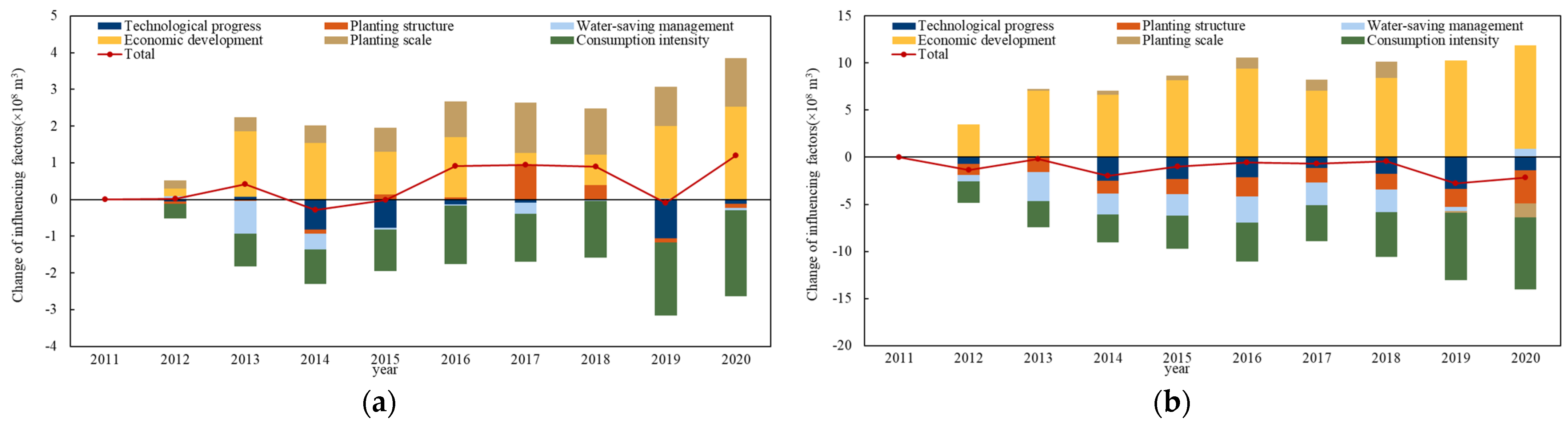
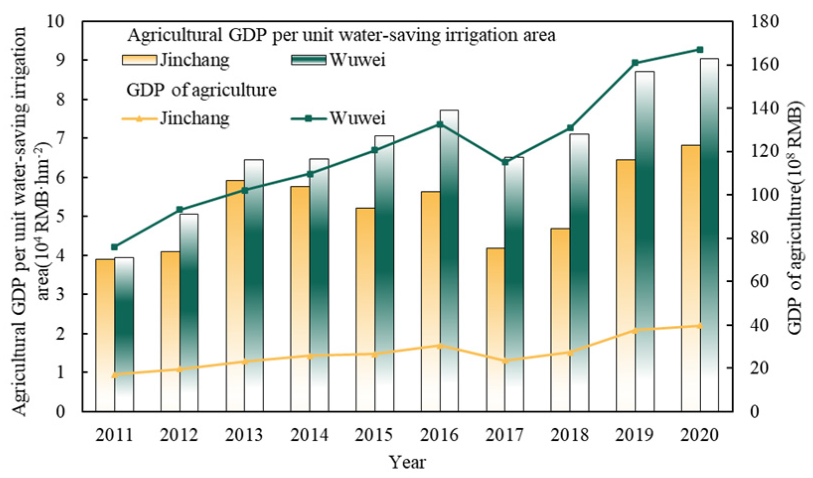
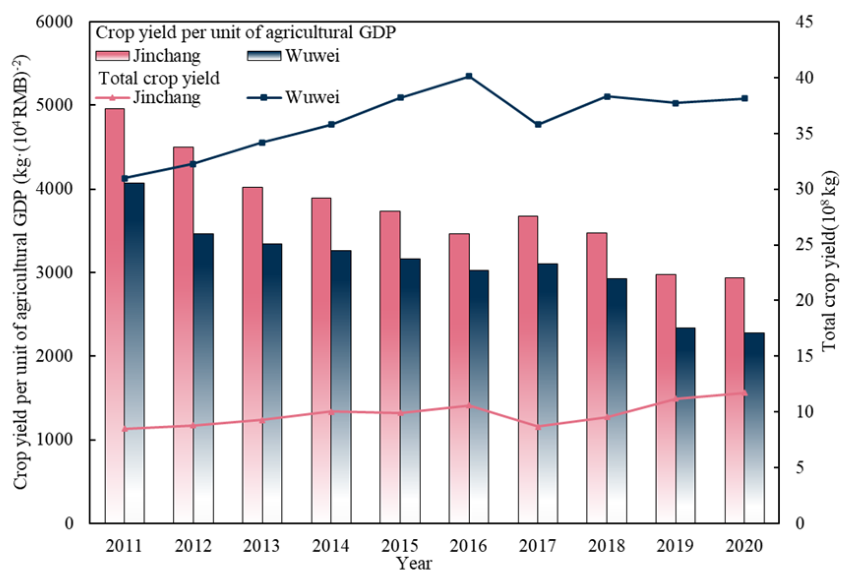
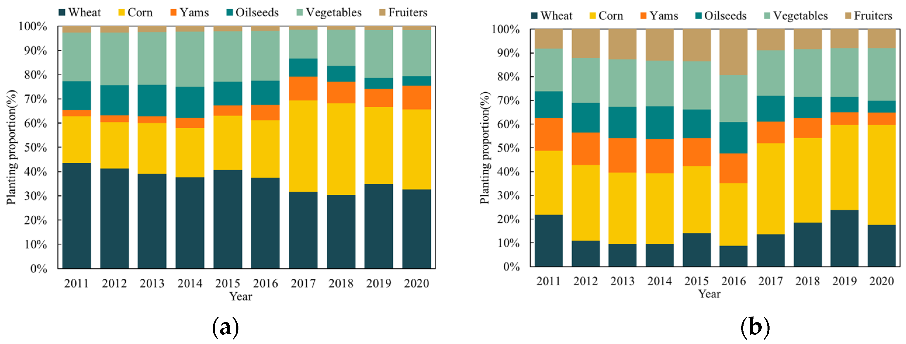
3.2. Decomposition Analysis

Figure 3 shows the changes in the driving effects of the six factors over the past 10 years. Economic development was the largest positive driver, accounting for 29% and 43% of the absolute contribution of the drivers in JC and WW, respectively, and driving the increase in irrigation water demand by 11.97 × 10⁸ m³ and 71.46 × 10⁸ m³, respectively. Consumption intensity was the largest negative driver, accounting for 31% and 23% of the absolute contribution of the drivers in JC and WW, driving a reduction in irrigation water demand of 12.16 × 10⁸ m³ and 39.06 × 10⁸ m³, respectively. Planting scale, planting structure, technological progress, and water conservation management have bidirectional driving effects. The planting scale was positively driven in JC, with an absolute average contribution of 20%, driving an increase of 7.71 × 10⁸ m³ in JC’s irrigation water demand. Planting scale in WW has a two-way driving role; the absolute average contribution rate was only 4%. The absolute average contribution of planting structure in JC and WW was 6% and 10%, respectively, and the planting structure was negatively driven in both regions, except in 2017–2018, when it was positively driven in JC. The absolute average contribution of technological progress and water-saving management was 8% and 6% in JC, and 9% and 11% in WW; both of them showed a negative driving effect for most of the time, and the negative driving effect was larger in WW than JC.

The results of the LMDI decomposition showed that the economic development effect contributed the most to promote the increase in irrigation water demand in JC and WW during the study period. The contribution of economic development to irrigation water demand was higher in WW than in JC. From 2011 to 2020, the agricultural Gross Domestic Product (GDP) per unit of water-efficient irrigated area demonstrated a substantial increase. In the case of JC, there was a 76% increase, while WW experienced a 129% increase. Additionally, the overall agricultural GDP witnessed a significant growth, with JC observing a 133% increase and WW experiencing a 120% increase during the same period (Figure 4). The proportion of rural population in WW is twice as much as that of JC, but the domestic production was always only 1.64 times as much as that of JC; JC has a developed economy and a complex economic structure, and the GDP of the first industry accounts for less than 10%, while the proportion of the first industry in WW is about 30%. JC is dominated by industrial production [38], and WW’s economic development is highly dependent on agriculture. Zeng W in the decomposition of crop water resource use (WRU) found that the level of the economy is the largest contributor to the growth of WRU [25], and that the driving effect is more pronounced in the areas with a more agriculture-dependent economy.

Consumption intensity was the most important contributor to the reduction in irrigation water demand over the study period. Improvements in crop varieties, agricultural productivity, and the related production management levels reduce the amount of biomass consumed to produce the same output value, and a reduction in agricultural consumption intensity also contributes to a reduction in irrigation water demand. The contribution of consumption intensity to irrigation water demand was greater in JC than in WW. From 2010 to 2020, the crop production per RMB 10,000 of agricultural GDP decreased by 41% and 44% in JC and WW, respectively, and the total production increased by 38% and 23%, respectively (Figure 5). The intensity of agricultural consumption in JC was greater than that in WW, and therefore, the driving contribution of consumption intensity to irrigation water demand was greater than that in WW. Water-use intensity is an important factor that inhibits the growth of crop water resource use (WRU) [25], and slowing down consumption intensity can effectively reduce water demand [14].

Cultivation structure influences changes in irrigation water demand. The rational optimization of cropping structures can reduce irrigation water requirements to some extent without sacrificing food production [16].As shown in Figure 6, during the period of 2011–2020, the percentage of wheat, corn, yams, oilseeds, vegetables, and fruiters planted in JC changed from 44:19:2:12:20:3 in 2011 to 32:33:10:4:19:2 in 2020, with average rates of change of 1%, 12%, 24%, −7%, 4%, and −2%. The proportion of each crop in WW was uniform, and the proportion of wheat, corn, yams, oilseeds, vegetables, and fruiters cultivation changed from 22:27:14:11:18:8 in 2011 to 18:42:5:5:22:8 in 2020, with average rates of change of 3%, 5%, −10%, −8%, 1%, and 3%. The average sowing share of wheat, which is highly water-intensive, was 33%, and the increase in the areas sown to maize in JC was 75% in 2017, and the sudden change in the cropping structure is the main reason for the positive drive in the irrigation water demand in JC [39]. The planting structure in WW is constantly rationalizing [40], so the planting structure is contributing more and more to the negative drive of irrigation water demand in WW. Increased rationalization and the stability of planting structures drive reduced irrigation water requirements.

Cropping size is the second most positive driver of irrigation water demand in JC, and it is a two-way driver in WW. As shown in Figure 7(a), during the period of 2011–2020, the crop sown areas in JC showed an upward trend, with an average rate of change of 4% during the study period. The average rate of change in the crop sown areas in WW was −1%, as shown in Figure 7(b), the rates of change in the planting scale in WW reached −12% and −10% in 2019 and 2020, respectively, and the reduction in crop sown areas causes a reduction in irrigation water demand, which creates a negative driving effect on irrigation water demand in WW, and a positive driving effect in all other years.

There is a rebound effect of technological progress and water conservation management effects on irrigation water demand [11,41]. Technological progress and water-saving management effects have a negative driving effect on irrigation water demand. In 2013, 2014, and 2017, the negative driving contribution of the water conservation management effect to irrigation water demand in JC was at 22%, 10%, and 7%, and the proportion of water-saving irrigated areas to the irrigated areas was at 68%, 75%, and 78% in these three years, respectively. In WW, from 2013 to 2018, the negative driving contribution rate of the water conservation management effect fluctuated and decreased from 20% to 12%, and the proportion of water-saving irrigated areas to the sown areas fluctuated and increased from 73% to 77%. In the case of the water-saving irrigated areas with shares of less than 80%, the negative driving effect is greater in the years when the share of water-saving irrigated areas is smaller. However, this changed in years when the share of water-saving irrigated areas was more than 80%. The negative driving contribution of water-saving management effects in JC was between 1% and 6%, while the negative driving contribution of water-saving irrigation in WW was between 2% and 8%, and the water-saving management effects even had a positive driving effect in WW in 2020, when the share of water-saving irrigated areas reached 97% in that year. These negative driving effects of water conservation management on irrigation water demand are all lower than the years when the proportion of water-saving irrigated areas was below 80%. The spatial and temporal comparisons revealed that the effect of water-saving management had a larger negative driving effect when the percentage of water-saving irrigated areas was less than 80%, and when the percentage of water-saving irrigated areas was more than 80%, the negative driving effect of water-saving management on irrigation water demand was smaller than that of irrigation, or even increased. This is due to the fact that the increase in water-saving irrigation areas requires the consumption of lot of water at the same time, and the technical effect of water saving is not enough to offset the scale effect of the increase in irrigated area; the larger the areas of water-saving irrigation, the smaller the negative driving effect on irrigation water demand, with the potential for a positive driving effect. In addition, efficient irrigation technologies such as sprinkler and drip irrigation save water while increasing output, and increased output means more water consumption. Therefore, it is necessary to improve the level of water-saving irrigation technology and the efficiency of water-saving irrigation in water-saving irrigation management, and blindly expanding the scale of water-saving irrigation may be counterproductive.

4. Conclusions

This study provides a comparative analysis of the drivers of agricultural irrigation water demand in water-scarce regions with different levels of irrigated agricultural development. In JC, which has a higher level of irrigation, the absolute contributions of consumption intensity, economic development, and planting scale, which are the main drivers of irrigation water demand, accounted for 31%, 29%, and 20%, respectively. In WW, which has a lower level of irrigation, the main drivers of irrigation water demand were 43%, 23%, and 11% of the absolute contribution of economic development, consumption intensity, and water-saving management, respectively. The driving direction of the driving factors affecting irrigation water demand is both positive and negative, the positive driving factors are economic development and planting scale, and the negative driving factors are consumption intensity, planting structure, water conservation management, and technological progress. The positive and negative effects are not the same in different regions; the positive driving contribution of planting scale to irrigation water demand in JC is larger than that in WW, and the negative driving contribution of planting structure to irrigation water demand in WW is larger than that in JC. The results of this study are important guidance for agricultural management and water-saving irrigation development in JC and WW. In summary, our recommendations, as outlined in the study conducted in JC and WW, are as follows:

(1)

The optimization of planting structure and the implementation of water-saving irrigation practices to enhance food security;

(2)

The promotion and development of advanced water-saving irrigation technologies such as seepage irrigation and micro-sprinkler irrigation to conserve water;

(3)

The appropriate control of the proportion of grain crops versus cash crops;

(4)

The expansion of planting areas dedicated to low-water-consuming crops.

Through these measures, we aim to address the challenges related to water scarcity and ensure sustainable agricultural practices for the future.

Changes in the proportion of water-saving irrigated areas to sown areas have a substantial influence on irrigation water demand. It is important to note that there is an observable rebound effect when this proportion surpasses 80%. In addition, as the proportion increases, the effectiveness of water-saving management in reducing irrigation water demand gradually diminishes. This finding can effectively guide irrigation programs in water-scarce areas and improve the adaptability of irrigated agriculture in water-scarce areas. The development of irrigated agriculture in water-scarce areas needs to rely on the development of water-saving technology, and should not blindly expand the areas of water-saving irrigation. The obvious driving effects of economic development and consumption intensity on irrigation water demand in water-scarce areas need to be emphasized in the production layout of agriculture in water-scarce areas.

Economic development and consumption intensity are indirect factors that drive irrigation water demand, affecting irrigation water demand by influencing agricultural cultivation, technological development, and so on. Subsequent studies should focus on the driving mechanisms between economic development, consumption intensity, and irrigation water demand; quantitatively characterize the influence of economic development and consumption intensity on irrigation water demand; and establish response function relationships to provide useful information for the sustainable development of agriculture in water-scarce areas.

References

1. Doll, P. Impact of climate change and variability on irrigation requirements: A global perspective. Clim. Chang. 2002, 54, 269–293. [Google Scholar] [CrossRef]
2. Li, Y.T.; Zhang, Z.D.; Liu, S.L.; Cao, Z.; Ke, Q.; Chen, L.; Wang, G. Long-term responses in different karst agricultural production systems to farm management and climate change: A comparative prefecture-scale study in Southwest China. Agric. Ecosyst. Environ. 2023, 352, 108504. [Google Scholar] [CrossRef]
3. Sun, S.K.; Wu, P.T.; Wang, Y.B.; Zhao, X.; Liu, J.; Zhang, X. The impacts of interannual climate variability and agricultural inputs on water footprint of crop production in an irrigation district of China. Sci. Total Environ. 2013, 444, 498–507. [Google Scholar] [CrossRef] [PubMed]
4. Yang, L.; Yang, Y.; Feng, Z.; Zheng, Y. Effect of maize sowing area changes on agricultural water consumption from 2000 to 2010 in the West Liaohe Plain, China. J. Integr. Agric. 2016, 15, 1407–1416. [Google Scholar] [CrossRef]
5. Zhang, Y.; Guo, Y.; Shen, Y.; Qi, Y.; Luo, J. Impact of planting structure changes on agricultural water requirement in North China Plain. Chin. J. Eco-Agric. 2020, 28, 1407–1416. (In Chinese) [Google Scholar]
6. Gajic, L. Effect of irrigation regime on yield, harvest index and water productivity of soybean grown under different precipitation conditions in a temperate environment. Agric. Water Manag. 2018, 210, 224–231. [Google Scholar] [CrossRef]
7. Jin, W.; Liu, S.S.; Zhang, K.; Kong, W. Influence of Agricultural Production Efficiency on Agricultural Water Consumption. J. Nat. Resour. 2018, 33, 1326–1339. (In Chinese) [Google Scholar]
8. Nechifor, V.; Winning, M. Projecting irrigation water requirements across multiple socio-economic development futures—A global CGE assessment. Water Resour. Econ. 2017, 20, 16–30. [Google Scholar] [CrossRef]
9. Zou, M.Z.; Kang, S.Z.; Niu, J.; Lu, H. A new technique to estimate regional irrigation water demand and driving factor effects using an improved SWAT model with LMDI factor decomposition in an arid basin. J. Clean. Prod. 2018, 185, 814–828. [Google Scholar] [CrossRef]
10. Lopez-Nicolas, A.; Pulido-Velazquez, M.; Macian-Sorribes, H. Economic risk assessment of drought impacts on irrigated agriculture. J. Hydrol. 2017, 550, 580–589. [Google Scholar] [CrossRef]
11. Xu, H.; Li, T.; Song, J. Estimation, driving factors, and regional differences of agricultural irrigation water rebound effect in arid areas: Examples of five provinces in northwestern China. Resour. Sci. 2017, 43, 1808–1820. (In Chinese) [Google Scholar]
12. Feng, L.; Chen, B.; Hayat, T.; Alsaedi, A.; Ahmad, B. The driving force of water footprint under the rapid urbanization process: A structural decomposition analysis for Zhangye city in China. J. Clean. Prod. 2017, 163, S322–S328. [Google Scholar] [CrossRef]
13. Lankford, B.; Pringle, C.; Mccosh, J.; Shabalala, M.; Hess, T.; Knox, J.W. Irrigation area, efficiency and water storage mediate the drought resilience of irrigated agriculture in a semi-arid catchment. Sci. Total Environ. 2023, 859, 160263. [Google Scholar] [CrossRef] [PubMed]
14. Ma, W.J.; Meng, L.H.; Wei, F.L.; Opp, C.; Yang, D. Sensitive Factors Identification and Scenario Simulation of Water Demand in the Arid Agricultural Area Based on the Socio-Economic-Environment Nexus. Sustainability 2020, 12, 3996. [Google Scholar] [CrossRef]
15. Guo, B.; Li, W.H.; Guo, J.Y.; Chen, C. Risk Assessment of Regional Irrigation Water Demand and Supply in an Arid Inland River Basin of Northwestern China. Sustainability 2015, 7, 12958–12973. [Google Scholar] [CrossRef]
16. Zhang, L.; Li, M.N.; Zhang, J.X.; Chen, F.; Lei, Y. Quantifying the food-water nexus and key drivers in China’s agricultural sector. J. Clean. Prod. 2023, 415, 137794. [Google Scholar] [CrossRef]
17. Xing, Z.K.; Ma, M.M.; Wei, Y.Q.; Zhang, X.; Yu, Z. A new agricultural drought index considering the irrigation water demand and water supply availability. Nat. Hazards 2020, 104, 2409–2429. [Google Scholar] [CrossRef]
18. Moorhead, J.E.; Gowda, P.H.; Marek, T.H.; Porter, D.O.; Howell, T.A.; Singh, V.P.; Stewart, B.A. Use of crop-specific drought indices for determining irrigation demand in the texas high plains. Appl. Eng. Agric. 2013, 29, 905–916. [Google Scholar]
19. Wang, L.; Xia, E.; Wei, Z.; Wang, W. Exploring the driving forces on sustainable energy and water use in China. Environ. Sci. Pollut. Res. 2022, 29, 7703–7720. [Google Scholar] [CrossRef]
20. Zhao, C.F.; Chen, B. Driving Force Analysis of the Agricultural Water Footprint in China Based on the LMDI Method. Environ. Sci. Technol. 2014, 48, 12723–12731. [Google Scholar] [CrossRef]
21. Li, C.; Jiang, T.T.; Luan, X.B.; Yin, Y.L.; Wu, P.; Wang, Y.; Sun, S.K. Determinants of agricultural water demand in China. J. Clean. Prod. 2021, 288, 125508. [Google Scholar] [CrossRef]
22. Zeng, W.; He, J.; Qiu, Y.; Cao, X. Unravelling the Temporal-Spatial Distribution of the Agricultural Water Footprint in the Yangtze River Basin (YRB) of China. Water 2021, 13, 2562. [Google Scholar] [CrossRef]
23. Zhang, S.; Su, X.; Singh, V.P.; Olaitan, A.O.; Xie, J. Logarithmic Mean Divisia Index (LMDI) decomposition analysis of changes in agricultural water use: A case study of the middle reaches of the Heihe River basin, China. Agric. Water Manag. 2018, 208, 422–430. [Google Scholar] [CrossRef]
24. Liu, X.; Peng, X.; Bai, L.; Gao, C. Study on Driving Factors of Agricultural Water in Hebei Province Based on Water Footprint. Chin. J. Agric. Resour. Egional Plan. 2021, 42, 188–198. (In Chinese) [Google Scholar]
25. Zeng, W.; Cao, X.C.; Huang, X.; Wu, M. Water resource use and driving forces analysis for crop production in China coupling irrigation and water footprint paradigms. Environ. Sci. Pollut. Res. 2022, 29, 36133–36146. [Google Scholar] [CrossRef]
26. Zhang, H.; Wang, H. Spatial and temporal characteristics of water requirement and water deficit of wheat in Gansu Province from 1967 to 2017. Arid Land Geogr. 2007, 42, 1094–1104. (In Chinese) [Google Scholar]
27. Zhang, H.; Wang, H.; Xu, C. Spatial and temporal characteristics of water requirement and water deficit of maize in Gansu Province from 1967 to 2017. Acta Ecol. Sin. 2015, 40, 1718–1730. (In Chinese) [Google Scholar]
28. Ling, T. Impacts of Environment Change on Agricultural Water Consumption in Shiyang River Basin in Arid Region of Northwest China; Northwest A&F University: Shaanxi, China, 2007. (In Chinese) [Google Scholar]
29. He, G. Analytical Study on Measurement and Analysis of Effective Utilization Coefficient of Gansu Agricultural Irrigation Water. Gansu Sci. Technol. 2015, 31, 49–50+80. (In Chinese) [Google Scholar]
30. Banerjee, S.; Chatterjee, S.; Sarkar, S.; Jena, S. Projecting Future Crop Evapotranspiration and Irrigation Requirement of Potato in Lower Gangetic Plains of India using the CROPWAT 8.0 Model. Potato Res. 2016, 59, 313–327. [Google Scholar] [CrossRef]
31. Geng, Q.L.; Zhao, Y.K.; Sun, S.K.; He, X.; Wang, D.; Wu, D.; Tian, Z. Spatio-temporal changes and its driving forces of irrigation water requirements for cotton in Xinjiang, China. Agric. Water Manag. 2023, 280, 108218. [Google Scholar] [CrossRef]
32. Alghassab, M.; Khan, Z.A.; Altamimi, A.; Imran, M.; Alruwaili, F.F. Prospects of Hybrid Energy in Saudi Arabia, Exploring Irrigation Application in Shaqra. Sustainability 2022, 14, 5397. [Google Scholar] [CrossRef]
33. Yetik, A.K.; Sen, B. Evaluation of the Impacts of Climate Change on Irrigation Requirements of Maize by CROPWAT Model. Gesunde Pflanz. 2023, 75, 1297–1305. [Google Scholar] [CrossRef]
34. Smith, M. A Computer Program for Irrigation Planning and Management; FAO: Rome, Italy, 1992. [Google Scholar]
35. Jin, Q.; Gui, D.; Gao, X.; Zeng, F.-J.; Xue, J.; Zhang, Q.-F. Water footprints of primary crop production in Xinjiang. Agric. Res. Arid Areas 2018, 36, 243–249. (In Chinese) [Google Scholar]
36. Ang, B.W.; Liu, F.L. A new energy decomposition method: Perfect in decomposition and consistent in aggregation. Energy 2001, 26, 537–548. [Google Scholar] [CrossRef]
37. Kaya, Y. Impact of carbon dioxide emission control on GNP growth: Interpretation of proposed scenarios. RIPCC Energy Ind. Subgr. Paris 1990. [Google Scholar]
38. Wang, L.; Chen, F. Change in water-use efficiency of irrigated areas before and after integrated management in Shiyang River Basin. Acta Ecol. Sin. 2018, 38, 3692–3704. (In Chinese) [Google Scholar]
39. Fang, G.; Chen, Y.; Li, Z. Variation in agricultural water demand and its attributions in the arid Tarim River Basin. J. Agric. Sci. 2018, 156, 301–311. [Google Scholar] [CrossRef]
40. Juan, X.; Xiaoling, S. Decomposition of influencing factors on irrigation water requirement based on LMDI method. Trans. Chin. Soc. Agric. Eng. (Trans. CSAE) 2018, 33, 123–131. (In Chinese) [Google Scholar]
41. Fang, L.; Wu, F.P.; Yu, Y.T.; Zhang, L. Irrigation technology and water rebound in China’s agricultural sector. J. Ind. Ecol. 2020, 24, 1088–1100. [Google Scholar] [CrossRef]
Figure 1. Overview of the study area.
Sustainability 15 14951 g001
Figure 2. Irrigation water demand, 2011–2020: (a) JC; (b) WW.
Sustainability 15 14951 g002
Figure 3. Irrigation water demand drivers 2011−2020: (a) JC; (b) WW.
Sustainability 15 14951 g003
Figure 4. Interannual changes in agricultural GDP per irrigated area and agricultural GDP in JC and WW, 2011−2020.
Sustainability 15 14951 g004
Figure 5. Interannual changes in crop production per unit of agricultural GDP and total crop production in JC and WW, 2011−2020.
Sustainability 15 14951 g005
Figure 6. Planting structure, 2011−2020: (a) JC; (b) WW.
Sustainability 15 14951 g006
Figure 7. Percentage of areas under water-saving irrigation and crop sowing, 2011−2020: (a) JC; (b) WW.
Sustainability 15 14951 g007