Coupling of Forest Carbon Densities with Landscape Patterns and Climate Change in the Lesser Khingan Mountains, Northeast China

Abstract

This research investigated the effects of the forest landscape composition and spatial distribution and local climate change’s lag effects on the carbon density of stands and provides a reference for optimizing the stand structure and sustainable management of forest resources in Xinqing District, Yichun City, Heilongjiang Province, China. Using second-class forest resource survey data of the Xinqing Forestry Bureau for 2007 and 2017, the forest carbon density, landscape pattern index and local forest climate were quantified by ArcGIS10.7, Fragstats4.2 and SPSS25, and a coupling coordination degree model was constructed to reflect their correlations. The overall broadleaved mixed forest area was larger in the new green area, and the overall forest productivity had improved in the past ten years. Forest management gradually improved from nonforest to forest land, resulting in a high degree of fragmentation in the surrounding landscape. The coupling research on the forest carbon density and the forest landscape pattern index and local climate index showed that, overall, the landscape pattern and the impact of climate change on the forest carbon density had a positive interaction; adjustments and improvements can be made to the forest carbon density in the poor-condition area by combining specific situations of the landscape pattern and climate change.

1. Introduction

As an important natural resource on Earth, forests benefit the economy, ecology and society, and they are essential to human survival, economic development and social progress. Currently, global warming is an urgent issue that needs to be solved; CO₂ is considered to be the culprit of global warming, and carbon emission reduction has become the consensus of almost all countries in the world today [1]. The frequent occurrence of severe droughts and high-temperature events due to global warming [2,3] will threaten the survival of forests [4,5] and put the ecological, social and other services provided by forests at risk [6]. Forest ecosystems are the largest photosynthetic system in terrestrial ecosystems, occupying 80% of the aboveground carbon pool and 40% of the belowground carbon pool in terrestrial ecosystems. More than 90% of CO₂ exchange between terrestrial plants and the atmosphere is completed by storing carbon in trees and soil. This exchange helps balance the CO₂ concentration in the atmosphere and maintain the stability of the global temperature [7,8]. Forests are highly recognized by the international community as absorbers and reservoirs of CO₂ and as buffers against the impact of human activities or modern science and technology, and they play a role in regulating global warming [9,10].

Research on the forest carbon density first appeared in 1876. Ebermeyer proposed that research subjects include forest branches and litter, and his research results provided a theoretical basis for the development of forest carbon density. Forest inventory data contain information such as forest types, stand age, DBH, tree height and volume, which can be used to estimate the carbon density. The four commonly used methods are the conversion factor continuous method, average biomass method, volume-derived biomass method and biomass regression equation [11]. For the estimated carbon density, many scholars have studied its distribution and dynamic changes due to geographical and environmental factors. Smithwick and Hudiburg et al. showed that compared with other regions, the Northwest Pacific region of North America has the largest natural terrestrial carbon density potential [12,13]. However, with disturbances to altitude gradients, soil and climate change, there are great differences in the distribution of the carbon density [14]. To date, most studies on the stand carbon density have focused on its distribution characteristics, influencing factors and measurement methods, and few studies have focused on the coupling relationship related to the carbon density. On the basis of analyzing the spatial distribution and dynamic changes in carbon density, this study attempted to conduct a coupling analysis from the perspective of the landscape index and climate index.

In recent decades, with the rapid development of China’s economy, the impact of some human activities has exceeded the bearing capacity of the natural environment. Large-scale construction and mining activities have gradually caused the once-continuous natural landscape to become complex and discontinuous, resulting in an increase in landscape fragmentation [15,16,17]. The fragmented landscape will react to the ecosystem and eventually affect human life. Therefore, this study attempted to analyze the effects of the spatial distribution and structural changes in forest landscapes on forest productivity. To date, many scholars have studied landscape evaluation, dynamic changes and driving force factors. Hashem et al. showed that [18] changes in landscape patterns were positively correlated with changes in land use, and Jialing Wang et al. confirmed that [19] optimizing landscape patterns was beneficial to forest resource protection. Xun Liang et al.’s research results show that [20] their patch-generating land use simulation (PLUS) model can produce substantial guidance for managing future land use patterns with different development goals. Research on coupling relationships has mainly focused on the construction and stability analysis of forest landscape patch coupling networks, and their results show that the combination of the dynamic landscape scale and network coupling can solve the problem of promoting forest resilience at different spatial levels [21,22]. Tang et al.’s research on the coupling relationship between the stand carbon density and forest landscape pattern shows that [23] corresponding management measures can be formulated according to the coupling coordination degree, and targeted management can be carried out to improve the spatial allocation of stands and increase the carbon density of stands.

The interaction between climate change and forests can directly affect forest growth through meteorological elements and can mitigate climate change through forest management [24,25]. At present, many scholars focus on building various models to assess forest biomass and carbon density. Xiao He et al.’s results show that [26] the random forest (RF) algorithm can compensate for the shortcomings of traditional regression models in estimating stands’ biological carbon density and climate factors’ influences on it. Research on coupling has focused on coupled models of the local community climate and global climate. Churchill et al. improved [27] and evaluated the ability of the Europe-Mediterranean Centre for Climate Change Coupled Climate Model (CMCC-CM2) to reproduce today’s average climate and interannual variability in terms of major tropical and temperate models. In a coupling study of forest carbon density and climate change, Ghislain et al. analyzed [28] the relationship between them through coupling with a bioclimate envelope model, and the research results showed that annual precipitation and annual average temperature were the key variables in determining the forest carbon density.

Therefore, the purpose of this study was to provide a scientific basis and relevant theoretical reference for the rational distribution of forest resources, optimization of the landscape structure, sustainable development of forest resources and creation of a good ecological environment based on the forest carbon density in China’s Lesser Khingan Mountains. The specific goals were to (1) estimate the forest carbon density in 2007 and 2017 and analyze the spatial distribution and dynamic characteristics of the forest carbon density; (2) describe the dynamic evolution trend of forest landscape patterns in the study area; and (3) quantify and analyze the coupling coordination degree between the landscape pattern index, climate factor index and stand carbon density. The results suggest that the method of coupling coordination between different systems to regulate forest productivity can help identify the areas that need to be adjusted and improved on a large scale, formulate corresponding management measures and improve stands’ spatial allocation.

2. Materials and Methods

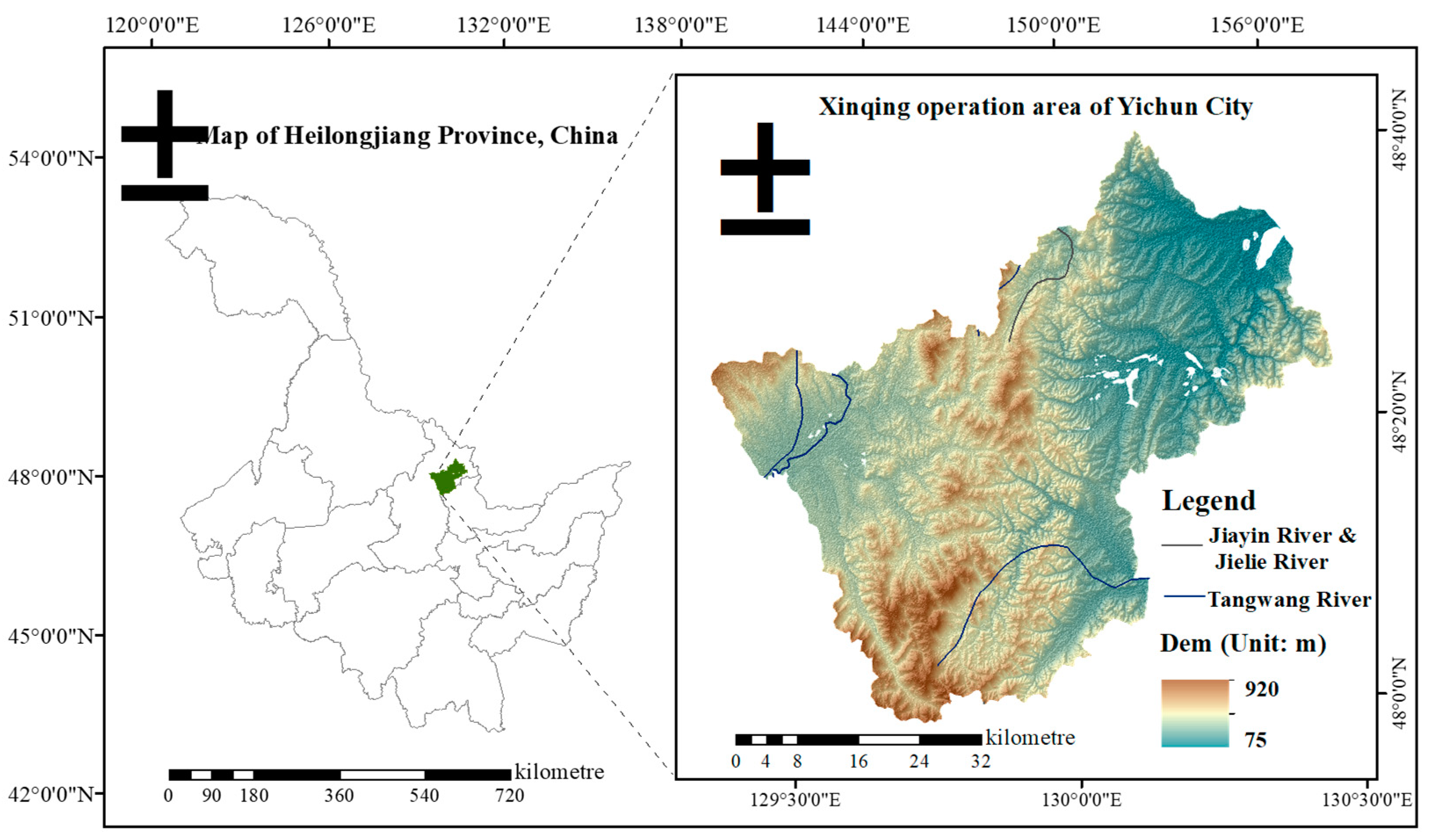
2.1. Study Area

Xinqing is in Yichun City, Heilongjiang Province, and it is also known as the hometown of China’s white-head crane. It is in the hinterland of the Lesser Khingan Mountains, the hometown of red pines, in northern Yichun. Its geographical coordinates are 129°20′ to 130°23′ E and 47°55′ to 48°40′ N. It borders Jiayin County and Hegang City in the east, Hongxing District in the west, Meixi in the south, and Tangwanghe District in the north. The Xinqing region is divided into two parts: an administrative region and an operation area. The current system integrates the government and enterprise of the Xinqing District People’s government and the Xinqing Forestry Bureau. In 2010, the State Forestry Administration designated the Xinqing Forestry Administration (Figure 1) as a pilot forest unit in China. As of 2018, its management area was 289,780 hectares. According to the forest classification management standard, the area of noncommercial forest is 201,969 hectares, accounting for 69.7% of the total area. The area of commercial forest is 65024 hectares, accounting for 22.4% of the total area. There are 931 species of higher plants in 163 families, including 169 species of bryophytes in 53 families, 49 species of ferns in 14 families, 7 species of gymnosperms in 2 families, and 706 species of angiosperms in 93 families.

2.2. Data Acquisition and Processing

2.2.1. Calculation of Carbon Density

With reference to the research of Tang Yiwu and Liu Liwu [23,29], according to the attributes of land class and dominant species in the vector data of the second-class survey of forest resources of the Xinqing Forestry Bureau, the area was divided into 8 categories, namely, Korean pine forest, larch forest, oak forest, birch grove, shrubbery, mixed broadleaf–conifer forest, mixed broadleaved forest and mixed coniferous forest, among which black birch and white birch were combined as birch grove. The coniferous forest of clouds and fir was classified as a mixed coniferous forest because of its small area, and the mixed broadleaved forest included other soft broadleaved and mixed broadleaved forests. The biomass model of the major tree species and stand types in the Northeast Forest region was studied by Dong Lihu [30] to build a stand biomass model, and the total biomass per unit was calculated (Table 1). The corresponding carbon content was obtained by referring to the carbon storage distribution and dynamic study of Heilongjiang published by Jia Weiwei [31], and the carbon density was obtained through multiplication with the previous results of total biomass per unit. The specific methods were as follows:

• Continuous function model formulas of forest biomass conversion coefficients

Table 1. Continuous function model formulas of biomass conversion coefficients.

WA = Wr + Ws + Wb + Wf *					(1)
Forest Types	Subitem	Formula	Forest Types	Subitem	Formula
Birch forest	root	Wr = (Dq/(−7.7814 + 5.2684 Dq)) V	Black birch forest	root	Wr = (Dq/(−11.7444 + 5.7857 Dq)) V
	trunk	Ws = (H/(−0.7161 + 1.7316 H)) V		trunk	Ws = (Dq/(3.0469 + 1.3313 Dq)) V
	branch	Wb = (H/(71.1504 + 2.3594 H)) V		branch	Wb = (Dq/(105.2694 − 1.7441 Dq))V
	leaf	Wf = (Dq/(52.1765 + 31.5260 Dq)) V		leaf	Wf = (Dq/(−133.4280 + 40.7349 Dq)) V
Korean pine forest	root	Wr = (H/(−7.4947 + 5.4000 H)) V	Oak forest	root	Wr = 0.2709 Dq−0.0224 H−0.0124 V
	trunk	Ws = (N/(369.6842 + 1.5593 N)) V		trunk	Ws = (Dq/(3.4101 + 1.1859 Dq)) V
	branch	Wb = 0.1087 Dq0.1196 H−0.1086 V		branch	Wb = (Dq/(70.6539 + 0.2149 Dq)) V
	leaf	Wf = 0.2835Dq−0.2446 H−0.2737 V		leaf	Wf = 0.0213 * Dq−0.0248 H0.2141 V
Mixed broadleaved forest	root	Wr = (H/(−6.0790 + 5.4717H)) V	Mixed coniferous forest	root	Wr = (Dq/(14.2890 + 4.8830 Dq)) V
	trunk	Ws = 0.5193 Dq0.1529 H−0.0981 V		trunk	Ws = (Dq/(0.6756 + 2.1000 Dq)) V
	branch	Wb = (Dq/(79.2051 + 1.2886 Dq)) V		branch	Wb = 0.0631 * Dq0.3538 H−0.2781 V
	leaf	Wf = (Dq/(−84.3635 + 42.2363 Dq)) V		leaf	Wf = (Dq/(−156.9210 + 43.4676 Dq)) V
Larch forest	root	Wr = (Dq/(44.2954 + 1.1820 Dq)) V	Larch plantation	root	Wr = (Dq/(43.1398 + 3.0221 Dq)) V
	trunk	Ws = 0.2638 * Dq0.6084 H−0.3052 V		trunk	Ws = (Dq/(11.8721 + 0.9735 Dq)) V
	branch	Wb = 0.0893 Dq0.5372 H−0.5798 V		branch	Wb = (Dq/(−14.7782 + 14.9115 Dq)) V
	leaf	Wf = (Dq/(−320.5650 + 69.0763 Dq)) V		leaf	Wf = (Dq/(−267.4450 + 57.5741 Dq)) V
Mixed broadleaf- conifer forest	root	Wr = (H/(−2.1908 + 5.6433 H)) V	Aspen forest	root	Wr = (Dq/(−7.7200 + 0.1178 Dq)) V
	trunk	Ws = (Dq/(−1.3193 + 2.0249 Dq)) V		trunk	Ws = (H/(−2.5225 + 2.0046 H)) V
	branch	Wb = (Dq/(58.0685 + 5.6768 Dq)) V		branch	Wb = (Dq/(107.0625 + 3.9071 Dq)) V
	leaf	Wf = (Dq/(−507.2690 + 78.1762 Dq)) V		leaf	Wf = (Dq/(13.5491 + 49.5804 Dq)) V

* Note: ${\mathrm{W}}_{\mathrm{A}}$ is the total biomass, ${\mathrm{W}}_{\mathrm{r}}$ is the root biomass, ${\mathrm{W}}_{\mathrm{s}}$ is the trunk biomass, ${\mathrm{W}}_{\mathrm{b}}$ is the branch biomass, ${\mathrm{W}}_{\mathrm{f}}$ is the leaf biomass, V is stock per hectare in the small class, D_q is the mean DBH of the stand within the small class, H is the average stand height within the small class, and N is the density of the stand in the small class. The carbon density formula of each stand is shown in the literature [30] P127–P129.

Table 1. Continuous function model formulas of biomass conversion coefficients.

WA = Wr + Ws + Wb + Wf *					(1)
Forest Types	Subitem	Formula	Forest Types	Subitem	Formula
Birch forest	root	Wr = (Dq/(−7.7814 + 5.2684 Dq)) V	Black birch forest	root	Wr = (Dq/(−11.7444 + 5.7857 Dq)) V
	trunk	Ws = (H/(−0.7161 + 1.7316 H)) V		trunk	Ws = (Dq/(3.0469 + 1.3313 Dq)) V
	branch	Wb = (H/(71.1504 + 2.3594 H)) V		branch	Wb = (Dq/(105.2694 − 1.7441 Dq))V
	leaf	Wf = (Dq/(52.1765 + 31.5260 Dq)) V		leaf	Wf = (Dq/(−133.4280 + 40.7349 Dq)) V
Korean pine forest	root	Wr = (H/(−7.4947 + 5.4000 H)) V	Oak forest	root	Wr = 0.2709 Dq−0.0224 H−0.0124 V
	trunk	Ws = (N/(369.6842 + 1.5593 N)) V		trunk	Ws = (Dq/(3.4101 + 1.1859 Dq)) V
	branch	Wb = 0.1087 Dq0.1196 H−0.1086 V		branch	Wb = (Dq/(70.6539 + 0.2149 Dq)) V
	leaf	Wf = 0.2835Dq−0.2446 H−0.2737 V		leaf	Wf = 0.0213 * Dq−0.0248 H0.2141 V
Mixed broadleaved forest	root	Wr = (H/(−6.0790 + 5.4717H)) V	Mixed coniferous forest	root	Wr = (Dq/(14.2890 + 4.8830 Dq)) V
	trunk	Ws = 0.5193 Dq0.1529 H−0.0981 V		trunk	Ws = (Dq/(0.6756 + 2.1000 Dq)) V
	branch	Wb = (Dq/(79.2051 + 1.2886 Dq)) V		branch	Wb = 0.0631 * Dq0.3538 H−0.2781 V
	leaf	Wf = (Dq/(−84.3635 + 42.2363 Dq)) V		leaf	Wf = (Dq/(−156.9210 + 43.4676 Dq)) V
Larch forest	root	Wr = (Dq/(44.2954 + 1.1820 Dq)) V	Larch plantation	root	Wr = (Dq/(43.1398 + 3.0221 Dq)) V
	trunk	Ws = 0.2638 * Dq0.6084 H−0.3052 V		trunk	Ws = (Dq/(11.8721 + 0.9735 Dq)) V
	branch	Wb = 0.0893 Dq0.5372 H−0.5798 V		branch	Wb = (Dq/(−14.7782 + 14.9115 Dq)) V
	leaf	Wf = (Dq/(−320.5650 + 69.0763 Dq)) V		leaf	Wf = (Dq/(−267.4450 + 57.5741 Dq)) V
Mixed broadleaf- conifer forest	root	Wr = (H/(−2.1908 + 5.6433 H)) V	Aspen forest	root	Wr = (Dq/(−7.7200 + 0.1178 Dq)) V
	trunk	Ws = (Dq/(−1.3193 + 2.0249 Dq)) V		trunk	Ws = (H/(−2.5225 + 2.0046 H)) V
	branch	Wb = (Dq/(58.0685 + 5.6768 Dq)) V		branch	Wb = (Dq/(107.0625 + 3.9071 Dq)) V
	leaf	Wf = (Dq/(−507.2690 + 78.1762 Dq)) V		leaf	Wf = (Dq/(13.5491 + 49.5804 Dq)) V

* Note: ${\mathrm{W}}_{\mathrm{A}}$ is the total biomass, ${\mathrm{W}}_{\mathrm{r}}$ is the root biomass, ${\mathrm{W}}_{\mathrm{s}}$ is the trunk biomass, ${\mathrm{W}}_{\mathrm{b}}$ is the branch biomass, ${\mathrm{W}}_{\mathrm{f}}$ is the leaf biomass, V is stock per hectare in the small class, D_q is the mean DBH of the stand within the small class, H is the average stand height within the small class, and N is the density of the stand in the small class. The carbon density formula of each stand is shown in the literature [30] P127–P129.

2.

Carbon density calculation of shrubbery

According to relevant research [32,33], the biomass per unit area of shrubbery was 19.67 t/hm², and the carbon content was 0.5.

$${\mathrm{B}}_{\mathrm{S}}={\mathrm{B}}_{\mathrm{unos}}\times {\mathrm{A}}_{\mathrm{s}}$$

(2)

where B_s represents the biomass of shrubbery in units of t, B_unos represents the biomass per unit area of shrubbery in units of t/hm², and A_s represents the area of shrubbery in units of hm².

3.

Calculation of forest carbon density

The average carbon content of the main tree species was multiplied by the estimated unit biomass to obtain the carbon density of the trees for the stand type. The average carbon contents of the major tree species are listed below (

Table 2. Average carbon content of the major tree species in the Northeast Forest region.

Forest Types	Average Carbon Content *	Stand Type	Average Carbon Content *
Spruce	0.4804	Fir	0.4805
Oak	0.453	Aspen	0.445
Black birch	0.4562	White birch	0.4656
Red pine plantation	0.4809	Natural red pine	0.4881
Larch plantation	0.4674	Natural larch	0.4742
Mixed broadleaved forest	0.453	Mixed coniferous forest	0.4802
Mixed broadleaf–conifer forest	0.458

* Note: The average carbon density of tree species is shown in the literature [31] P7.

).

2.2.2. Extraction of Landscape Pattern Index

In this study, the horizontal landscape pattern index was calculated and assigned to the center of each window using the moving-window method module in Fragstats 4.2 software. The spatial distribution map of each landscape pattern index was obtained by processing the map algebra module in ArcGIS 10.7 software. The dynamic evolution direction of the landscape pattern in the study area in the past ten years was analyzed, and the value-to-point data of the forest part of the index distribution map of the landscape patterns were extracted. To avoid using redundant information to describe the landscape heterogeneity characteristics more completely, commonly used landscape pattern indices were selected: area-weighted mean shape index (SHAPE_AM), patch density (PD), landscape shape index (LSI), patch area mean (AREA_MN), contagion index (CONTAG), aggregation index (AI), splitting index (SPLIT), Shannon’s diversity index (SHDI) and Shannon’s evenness index (SHEI). In total, 9 indicators were used to measure the characteristics of the forest landscape pattern in the Xinqing Forestry Bureau.

2.2.3. Extraction of the Climate Index from the Forest Bureau

The meteorological values of national meteorological stations from 2002 to 2006 and 2012 to 2016 were downloaded from the annual dataset of surface climate data in China, and the data included the average temperature, average air pressure, average water vapor pressure, average relative humidity, maximum wind speed, maximum atmospheric pressure, maximum air pressure, maximum temperature, daily precipitation and precipitation at 20:00. With the help of the ANUSPLIN plug-in, spatial meteorological interpolation was carried out for the study area and the surrounding area, and the raster data map of each meteorological factor was cropped.

2.2.4. The Coupling Coordination Degree Model

In this study, the coupling and coordination degree of three sets of systems are discussed: (1) carbon density of the stand and integrated landscape pattern index (CDOS-ILPI system), (2) carbon density of the stand and integrated local climate index (CDOS-CLCI system) and (3) carbon density of the stand and integrated landscape pattern index and integrated local climate index (CDOS-ILPI-CLCI system). To ensure the accuracy of the research results, it is necessary to adopt the positive impact (Formula (3)) and reverse impact (Formula (4)) formulas for each index to standardize the data and eliminate their influence on the same unit of measurement [34]. The formulas are as follows:

$${\mathrm{X}}_{\mathrm{i}\mathrm{j}}=\frac{{\mathrm{x}}_{\mathrm{i}\mathrm{j}}-\mathrm{m}\mathrm{i}\mathrm{n}\left\{{\mathrm{x}}_{\mathrm{i}\mathrm{j}}\right\}}{\mathrm{m}\mathrm{a}\mathrm{x}\left\{{\mathrm{x}}_{\mathrm{i}\mathrm{j}}\right\}-\mathrm{m}\mathrm{i}\mathrm{n}\left\{{\mathrm{x}}_{\mathrm{i}\mathrm{j}}\right\}},$$

(3)

$${\mathrm{X}}_{\mathrm{i}\mathrm{j}}=\frac{\mathrm{m}\mathrm{a}\mathrm{x}\left\{{\mathrm{x}}_{\mathrm{i}\mathrm{j}}\right\}-{\mathrm{x}}_{\mathrm{i}\mathrm{j}}}{\mathrm{m}\mathrm{a}\mathrm{x}\left\{{\mathrm{x}}_{\mathrm{i}\mathrm{j}}\right\}-\mathrm{m}\mathrm{i}\mathrm{n}\left\{{\mathrm{x}}_{\mathrm{i}\mathrm{j}}\right\}},$$

(4)

where ${\mathrm{X}}_{\mathrm{i}\mathrm{j}}$ represents the standardized value of indicator i for evaluation object j, ${\mathrm{x}}_{\mathrm{i}\mathrm{j}}$ represents the original value, and $\mathrm{m}\mathrm{a}\mathrm{x}\left\{{\mathrm{x}}_{\mathrm{i}\mathrm{j}}\right\}$ and $\mathrm{m}\mathrm{i}\mathrm{n}\left\{{\mathrm{x}}_{\mathrm{i}\mathrm{j}}\right\}$ indicate the maximum and minimum values, respectively.

The standardized landscape pattern index and local climate index were imported into SPSS25 software for principal component analysis to calculate their weights and composite indices. Liao et al. derived [35] the formula of the coupling coordination degree from the dispersion coefficient, but it is applicable to two subsystems. This formula has since been discussed by many scholars, among which Jiang et al. have corrected [36] the errors in the previous coupling formula and extended it to multiple subsystems. The formulas are as follows:

$${\mathrm{C}}_1=2\times \sqrt{\frac{{\mathrm{U}}_1\times {\mathrm{U}}_2}{{\left({\mathrm{U}}_1+{\mathrm{U}}_2\right)}^2}},$$

(5)

$${\mathrm{C}}_2=2\times \sqrt{\frac{{\mathrm{U}}_1\times {\mathrm{U}}_3}{{\left({\mathrm{U}}_1+{\mathrm{U}}_3\right)}^2}},$$

(6)

$${\mathrm{C}}_3={\left[\frac{{\mathrm{U}}_1\times {\mathrm{U}}_2\times {\mathrm{U}}_3}{{\frac{\left({\mathrm{U}}_1+{\mathrm{U}}_2+{\mathrm{U}}_3\right)}{3}}^3}\right]}^{\frac{1}{3}},$$

(7)

where C₁ represents the coupling degree of the CDOS-ILPI system, C₂ represents the coupling degree of the CDOS-CLCI system, C₃ represents the coupling degree of the CDOS-ILPI-CLCI system, U₁ represents the stand carbon density, U₂ represents the forest landscape pattern, and U₃ represents the local forest climate. A higher C value indicates a greater correlation between the three systems.

However, in some special cases, the coupling degree may not necessarily reflect the coordination degree between the three systems, and there may be a situation in which the development level of the three systems is low but the coupling degree is high. To prevent this scenario, a coupling coordination degree model was created [37]. The formula is as follows:

$$\mathrm{D}=\sqrt{\left(\mathrm{C}\times \mathrm{T}\right)},$$

(8)

$${\mathrm{T}}_1=\mathrm{a}{\mathrm{U}}_1+\mathrm{b}{\mathrm{U}}_2,$$

(9)

$${\mathrm{T}}_2=\mathrm{a}{\mathrm{U}}_1+\mathrm{c}{\mathrm{U}}_3,$$

(10)

$${\mathrm{T}}_2=\mathrm{d}{\mathrm{U}}_1+\mathrm{e}{\mathrm{U}}_2+\mathrm{f}{\mathrm{U}}_3,$$

(11)

where D represents the coupling coordination degree between systems, T1 represents the comprehensive development level of the CDOS-ILPI system, T2 represents the comprehensive development level of the CDOS-CLCI system, and T3 represents the comprehensive development level of the CDOS-ILPI-CLCI system. When a, b and c represent the weights of the stand carbon density, forest landscape pattern and forest local climate index in two systems, $\mathrm{a}=\mathrm{b}=\mathrm{c}=\frac{1}{2}$. When d, e and f represent the weights of the stand carbon density, forest landscape pattern and forest local climate index in three systems, $\mathrm{d}=\mathrm{e}=\mathrm{f}=\frac{1}{3}$ is selected for calculation, and a larger D value indicates that the systems are more coordinated. To further clarify the coupling coordination relationship between the stand carbon density, forest landscape patterns and local forest climate, the coupling coordination degree was graded, and the division results are shown in

Table 3. Level and standard of system coupling coordination degree.

D *	Coupling Coordination Degree Level
0 < D ≤ 0.3	Low coordinated coupling
0.3<D ≤ 0.5	Moderately coordinated coupling
0.5<D ≤ 0.8	Highly coordinated coupling
0.8<D ≤ 1	Extremely coordinated coupling

* Note: The grading standard of D is shown in reference [37] P1–P2.

.

3. Results

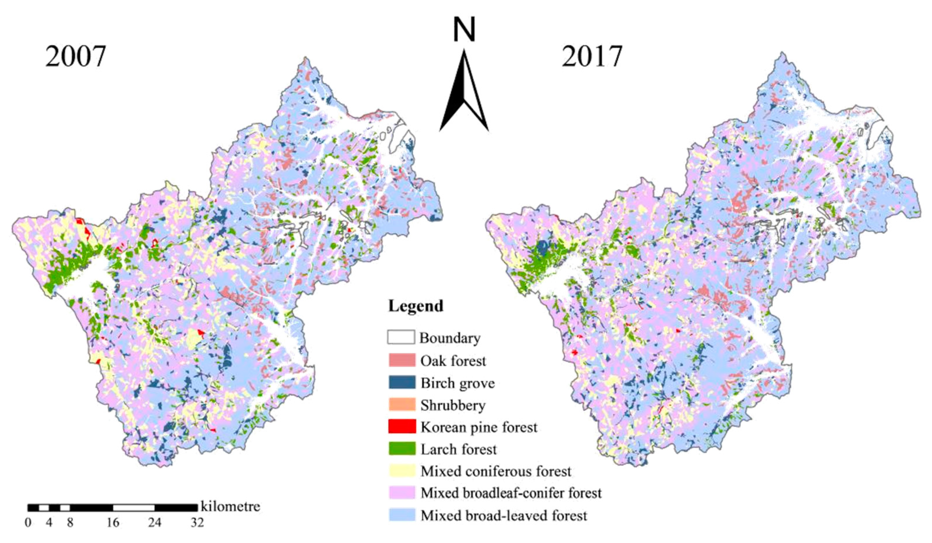
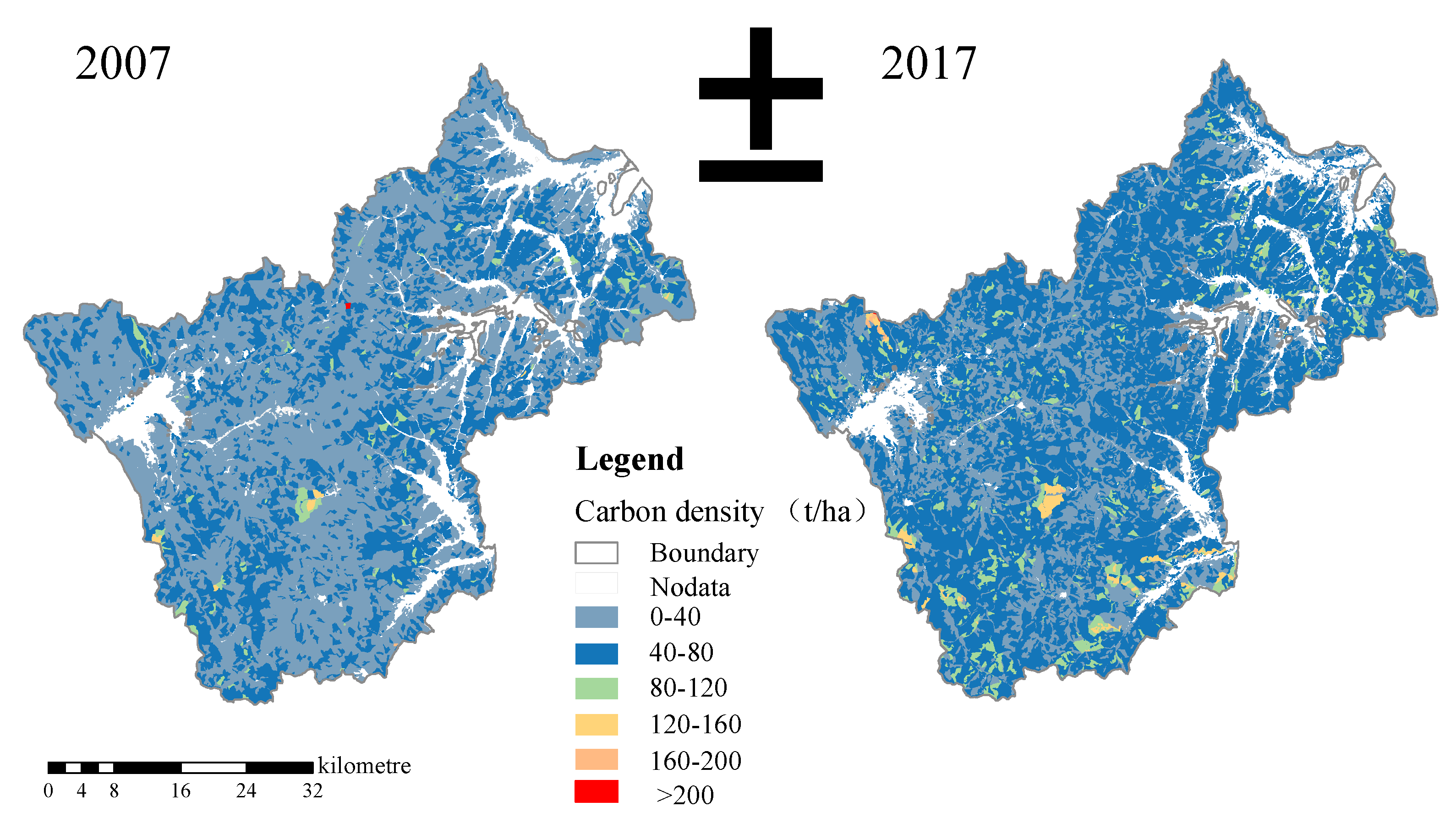
3.1. Results of Spatial Distribution of Forest Carbon Density

A variance analysis was performed on the obtained carbon density.

Table 4. Variance analysis of carbon storage and carbon density of different stand types.

	A Given Year	Sum of Squares	df	Mean Square	F	Significance
Carbon density	2007	256140.464	7	36591.495	119.277	0
	2017	432826.346	7	61832.335	151.164	0

shows that the significance level of the carbon density in 2007 and 2017 was 0.00 (both were less than 0.05), indicating that during this period, the carbon density differed significantly among different stand types. It was possible to further analyze the changes in the carbon density in the Xinqing Forestry Bureau over the past ten years. The spatial distribution of stand types in the study area is shown in Figure 2. A spatial visualization of the estimated two-stage stand carbon density is shown in Figure 3.

Based on

Table 5. Carbon storage and carbon density of different stand types in the Xinqing Forestry Bureau.

Forest Types	Area (hm2)		Specific Gravity		Dynamic Change (K, %)	Carbon Density (t/ha)
	2007	2017	2007	2017		2007	2017
Korean pine forest	726.04	322.52	0.29%	0.13%	−5.56%	68.8	84.23
Larch forest	16,510.21	12,106.51	6.55%	4.79%	−2.67%	30.7	53.03
Oak forest	9425.04	9231.42	3.74%	3.65%	−0.21%	52.2	63.17
Birch grove	12,702.61	13,989.59	5.04%	5.53%	1.01%	29.62	42.41
Mixed broadleaved forest	104,112.46	111,626.61	41.30%	44.14%	0.72%	38.29	51.84
Mixed coniferous forest	31,798.77	24,707.38	12.61%	9.77%	−2.23%	35.24	48.19
Mixed forest	76,647.44	80,829.05	30.40%	31.96%	0.55%	33.38	47.13
Shrubbery	183.42	82.2	0.07%	0.03%	−5.52%	9.84	9.84
Total	252,105.99	252,895.28	100.00%	100.00%		36.1	49.95

and Figure 2, among the different stand types in the study area, mixed broadleaved forest accounted for the largest area, and it was the dominant landscape type and was critical in the ecological environment’s regulation. In 2007, the area of mixed broadleaved forest was 104,112.46 hm^2, and in 2017, it was 111,626.61 hm², an increase of 7514.15 hm² and a dynamic change of 0.72%. Changing from 12,702.61 hm² in 2007 to 13,989.59 hm² in 2017, the dynamic change in birch forest was 1.01%.

The carbon density reflects carbon storage per unit area, and its value can better reflect the status of stand productivity. As shown in Figure 3, in 2017, the distribution range of carbon densities of 0–40 t/ha decreased compared to 2007, and the range of high values significantly increased. Carbon densities of 40–80 t/ha increased significantly, carbon densities of 80–120 t/ha increased in the northeast and south of the study area, and carbon densities of 120 t/ha and higher spread uniformly. From 2007 to 2017, the carbon density in the study area increased from 36.10 t/ha to 49.95 t/ha, an increase of 13.85 t/ha. The carbon densities of stands increased, except in shrub forest, and the greatest increase was in Larix forest, which increased from 30.7 t/ha in 2007 to 53.03 t/ha, an increase of 22.33 t/ha. The carbon density of red pine forest increased from 68.8 t/ha to 84.32 t/ha, but the area decreased by 2.2 times. Combined with the distribution area of red pine forests during the two periods, as shown in Figure 2, the reduced portion formed a mixed forest.

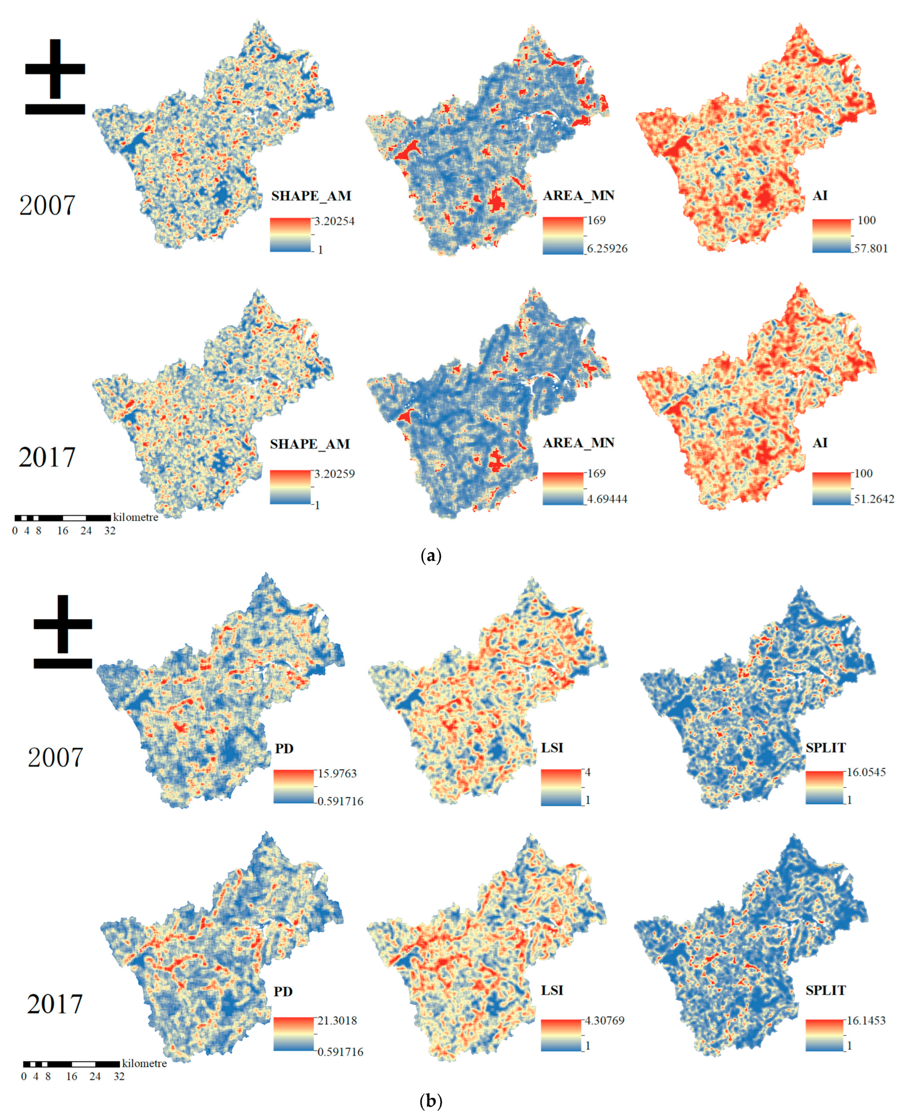
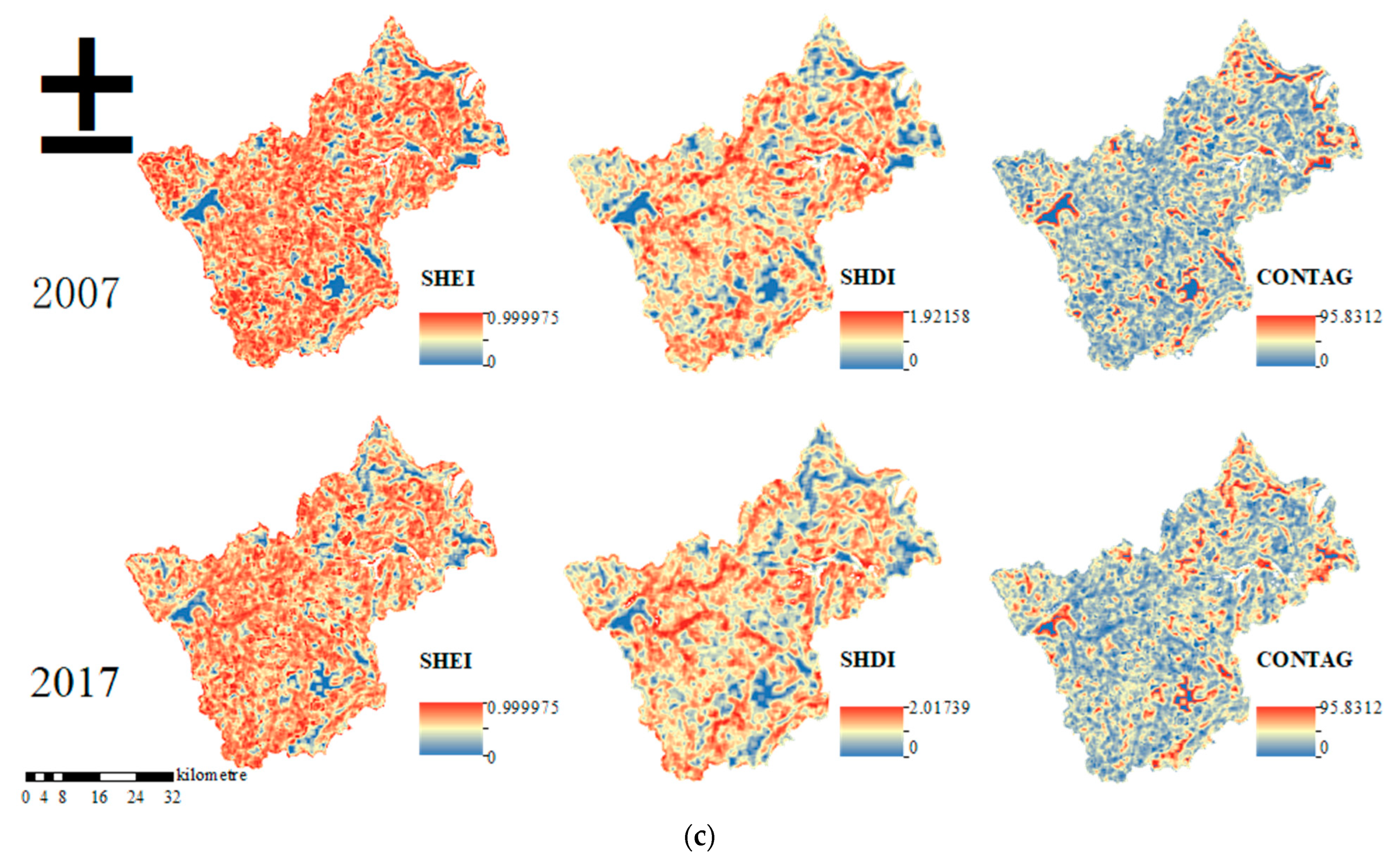
3.2. Results of the Moving-Window Method in Landscape Pattern Space Analysis

As shown in Figure 4, SHAPE_AM and AREA_MN were compared: the high value of the former was uniformly amplified from the inside to the outside, and the high value of the latter decreased significantly. The landscape index of the surrounding area near the nonforest area fluctuated greatly, indicating that this area was strongly influenced by human activities, and it was the main area with a high degree of fragmentation in the study area. For example, the values of PD and LSI increased significantly around nonforest land, and the AI showed a diffusion trend around nonforest land. Moreover, the AI increased significantly in the northern region but decreased in the northwestern region, indicating that the aggregation degree of the same stand type in the northern region increased with time. The nonforest patches were mostly distributed in the northeast, southeast and west of the study area. The patches were tightly clustered and less fragmented, and they had the lowest PD, LSI and SPLIT values, while the distribution of pixels with higher CONTAG values increased. The SHEI and SHDI of the area surrounding the nonforest area both decreased compared with those in 2007.

The extracted forest landscape pattern index in the study area was standardized by using the range method and then calculated by principal component analysis. The two principal components of the landscape pattern index in 2007 and 2017 were obtained, and the largest coefficients in each year were detected for the LSI and AI, indicating that in this study, the two indices had a greater impact on the comprehensive landscape pattern and could better present the overall situation. Their cumulative contribution rates reached 89.75% and 91.00%, respectively, and the weights of each index and the comprehensive landscape pattern index were calculated. The weight results are shown in

Table 6. Weight table of landscape pattern indicators in 2007 and 2017.

Index	Weights		Index	Weights		Index	Weights
	2007	2017		2007	2017		2007	2017
SPLIT	0.0820	0.0806	SHAPE_AM	0.1370	0.1261	CONTAG	0.1005	0.1109
SHEI	0.0972	0.0988	PD	0.0941	0.0981	AI	0.1464	0.1392
SHDI	0.1029	0.1071	LSI	0.1435	0.1386	AREA_MN	0.0963	0.1006

.

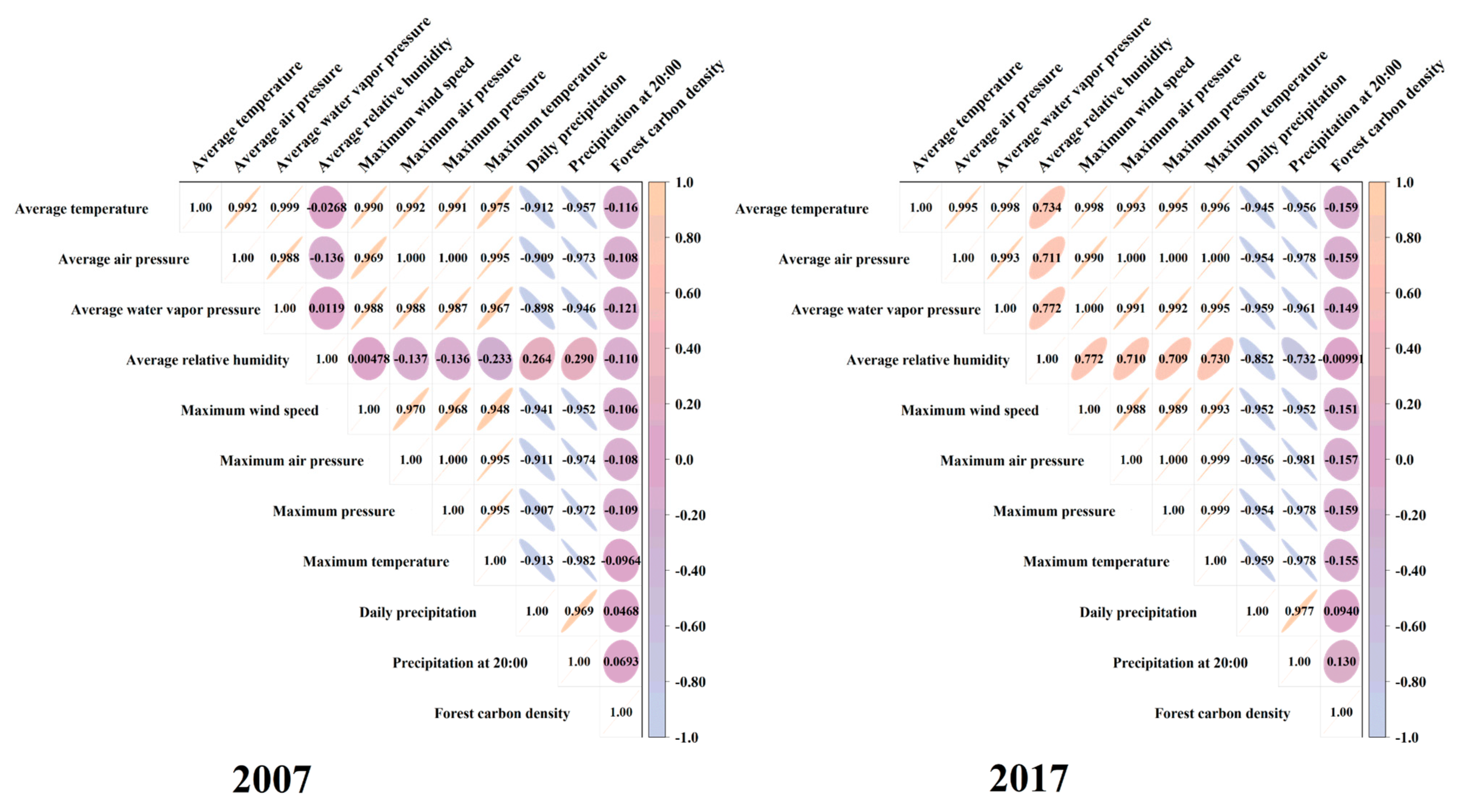
3.3. Results of Pearson Correlation Analysis for Screening Local Forest Climate Factors

Due to the lag effect of climate change on the carbon density of stands, the 5-year mean value of each index to analyze the impact of the carbon density of stands was selected. The 5-year mean value of the meteorological factor index of each small class was obtained, and Pearson correlation analysis was performed with the carbon density of the stand. Factors with a poor correlation were eliminated, and meteorological factors with a strong correlation with the carbon density of the stand were screened. Finally, seven indices, namely, average temperature, average air pressure, average water vapor pressure, maximum wind speed, maximum air pressure, maximum temperature and precipitation at 20:00, were retained as evaluation indices to evaluate the development of stand productivity.

The data range method of the selected meteorological factors was standardized, and the principal components of meteorological indicators in 2007 and 2017 were obtained through principal component analysis. The highest coefficients in each year were found for the mean pressure and maximum temperature, and their cumulative contribution rates reached 98.11% and 98.93%, respectively. Finally, the weights of each index and the comprehensive local climate level index were calculated. The Pearson correlation analysis results are shown in Figure 5, and the weight results are shown in

Table 7. Weight table of climate level indicators in 2007 and 2017.

Index		Average Air Pressure	Maximum Air Pressure	Average Temperature	Average Water Vapor Pressure	Maximum Temperature	Maximum Wind Speed	Precipitation at 20:00
Weights	2007	0.1439	0.1438	0.1436	0.1431	0.1428	0.1418	0.1410
	2017	0.1435	0.1435	0.1432	0.1432	0.1436	0.1428	0.1403

.

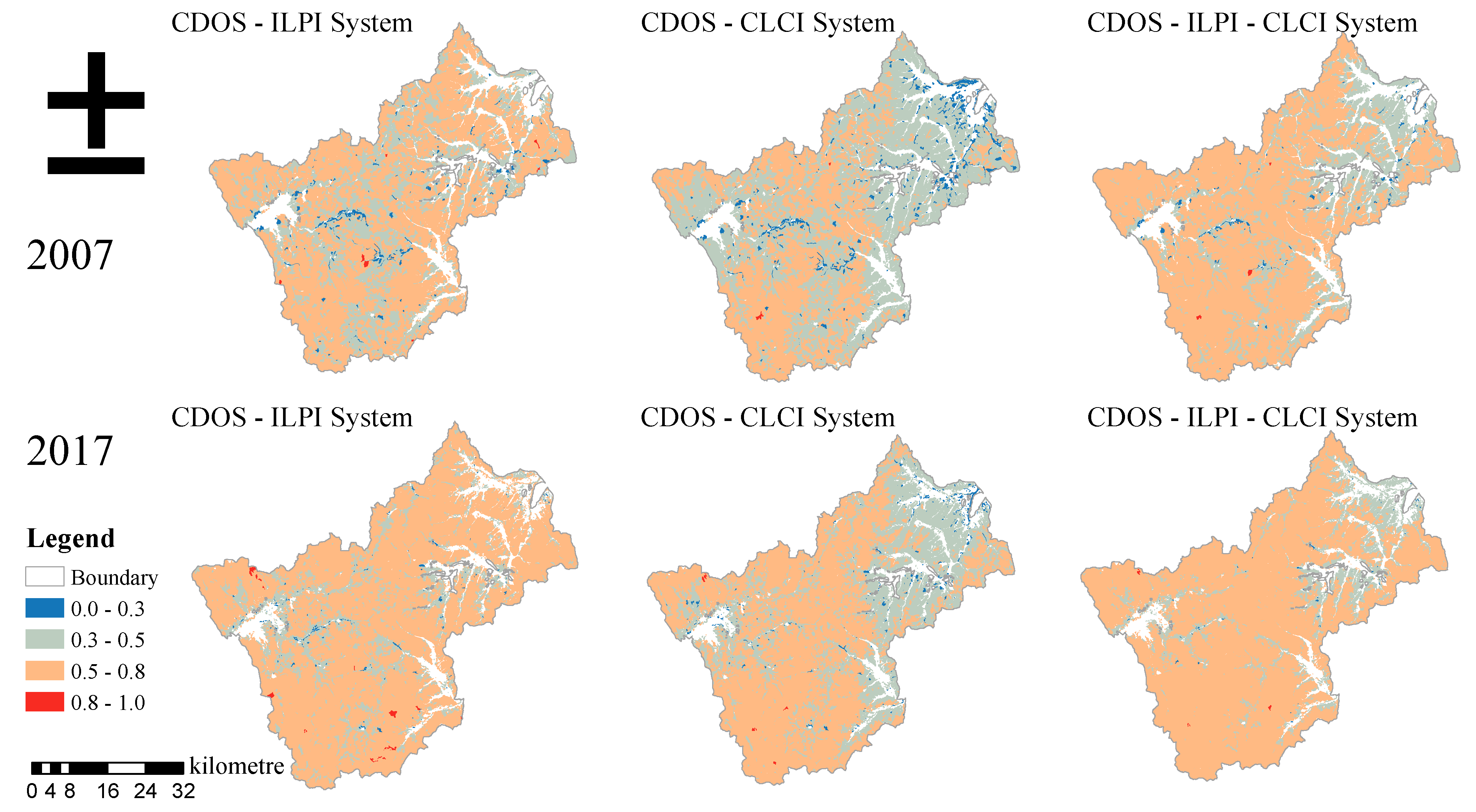
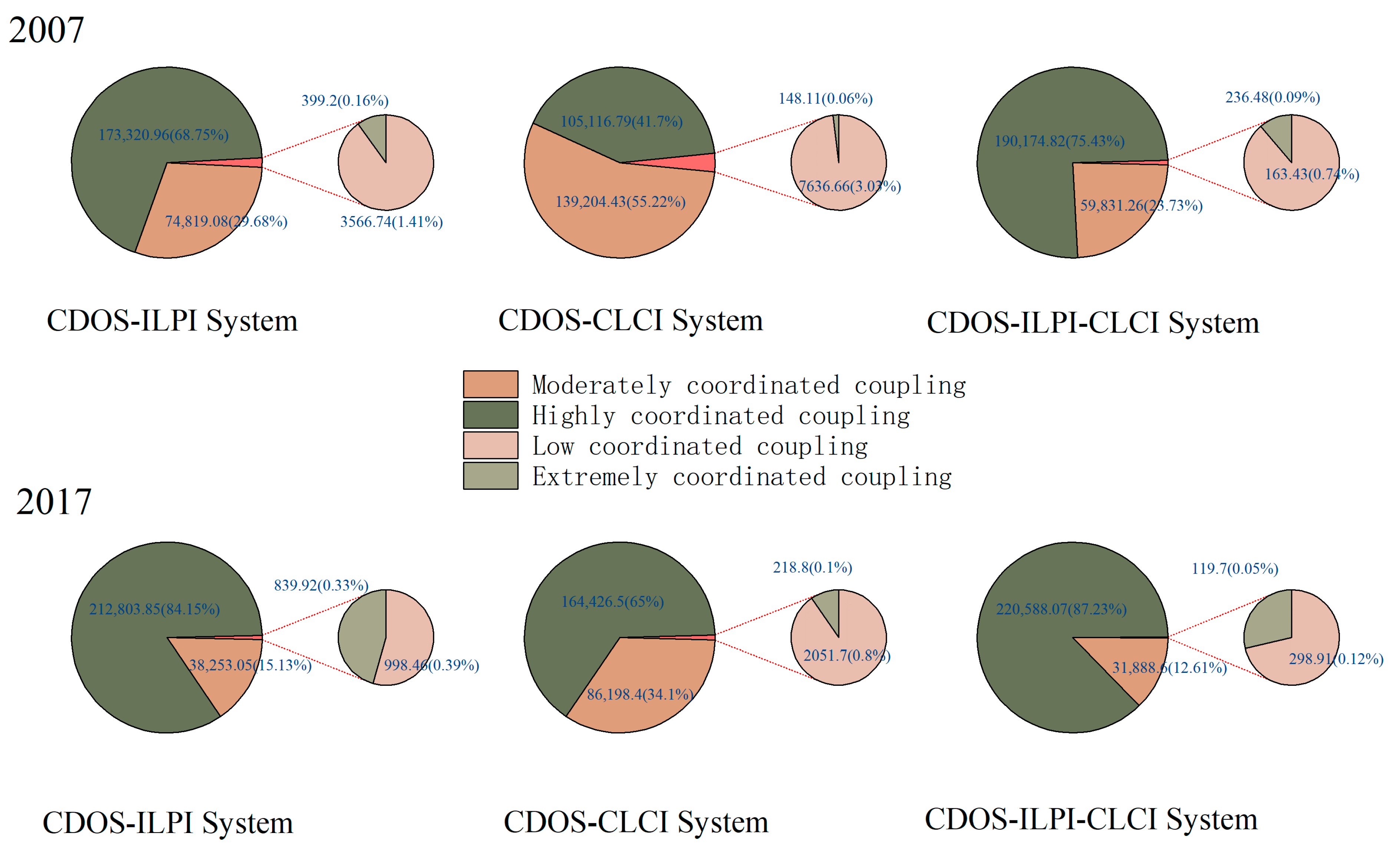
3.4. Results of the Spatial Distribution of the Coupling Coordination Degree

The integrated landscape pattern index, the integrated local climate index and the standardized data of stand carbon density were used to calculate the coupling coordination degree among the three systems: the CDOS-ILPI system, CDOS-CLCI system and CDOS-ILPI-CLCI system. Then, the coupling coordination degree was connected back to GIS to obtain a spatial visualization, as shown in Figure 6. The proportions of coupling areas with different coupling coordination degree levels in the three groups of systems were counted, as shown in Figure 7.

As shown in Figure 7, the high-coupling cooperative area of the CDOS-ILPI system in 2007 and 2017 was the largest, accounting for 68.75% and 84.15% of the total area, respectively, an increase of approximately 15.4 percentage points. The extreme-coupling coordination area increased from 0.16% to 0.33%, an increase of approximately 0.17 percentage points. The coupling-level area of the two phases of the CDOS-ILPI system was ranked as highly coordinated coupling > moderately coordinated coupling > low coordinated coupling > extremely coordinated coupling. In 2007, the coupling-level area of the CDOS-CLCI system was ranked as moderately coordinated coupling > highly coordinated coupling > low coordinated coupling > extremely coordinated coupling, while in 2017, the coupling-level area was ranked as highly coordinated coupling > moderately coordinated coupling > low coordinated coupling > extremely coordinated coupling. In 2007, the area of moderate coupling coordination was the largest, accounting for 55.22% of the total area, while in 2017, the area with high-coupling coordination was the largest, accounting for 65.02% of the total area. Under the joint action of climate factors and landscape patterns, the coupling-level area of the CDOS-ILPI-CLCI system was highly coordinated coupling > moderately coordinated coupling > low coordinated coupling > extremely coordinated coupling.

4. Discussion

4.1. Spatial Distribution and Characteristic Analysis of Carbon Density Based on Different Stand Types

In this study, a biomass conversion coefficient with a continuous function model was used to estimate the forest biomass in the study area in 2007 and 2017, and based on this, the model estimated the forest carbon density. The area, dynamic degree and carbon density distribution of each forest type over the past decade were studied. The results indicate (Table 6) that broadleaved mixed forest was the dominant tree species in this study area, and birch forest was the fastest-growing stand among all forest types. Second, the overall carbon density of the study area increased from 36.10 t/ha to 49.95 t/ha, with a significant increase in carbon density within the 40–80 t/ha range (Figure 3). In addition, the results showed that although the area of the Korean pine forest in the study area has decreased by half over the past decade, most areas where the carbon density of the Korean pine forest increased and the distribution range of the Korean pine forest decreased formed mixed forests.

The biomass model and carbon density used in this study can effectively estimate the biomass of various forest types in the Lesser Khingan Mountains region of Northeast China. Zhao Junfang et al. conducted a study on forest carbon storage in Northeast China from 1981 to 2002 and found that the spatial distribution of vegetation carbon density was characterized as high in the southeast and low in the northwest [38], which is consistent with the spatial distribution of carbon density in this study in 2007. Zhao Min et al. estimated the carbon density of forests in China to be 41.32 t/ha using the volume-derived biomass method based on the fourth forest inventory data of China (1989–1993), which is 5.22 t/ha higher than the carbon density in the study area in 2007. Zhang Xiaoyong et al. used remote sensing and deep learning to conduct a long-term analysis of forest carbon storage in Northeast China. The carbon density in 2019 was 21.35 t/ha higher than that in 2017. In this study, it was speculated that the reason for this phenomenon was influenced not only by forest growth but also by local factors, such as geographical conditions, climate change, precipitation and microbial activity. These different conditional factors form different forest types, and forest types and tree species significantly impact carbon estimation: therefore, different study area scales, data sources and estimation methods will lead to differences in the estimation results of the forest carbon density [11,39,40]. Overall, the forest carbon density in this study area has increased over time, which is consistent with the research results of many scholars. However, the data in this study are relatively outdated, and future research can be performed for further analyses after obtaining the latest survey data.

4.2. Spatial Characteristic Analysis of Landscape Patterns Based on the Moving-Window Method

The moving-window method was used to study the evolution of forest landscape patterns in the study area. The results showed that (Figure 4) there was significant heterogeneity in the landscape pattern of the study area, with an overall increase in forest landscape complexity, enhanced connectivity and increased biodiversity. The degree of aggregation of the same forest type in the northern region became closer over time, while there was a phenomenon of succession of forest types in the northwestern region. The aggregation degree of nonforest patches was tight, and the degree of fragmentation was relatively low. The landscape index of the surrounding area near nonforested areas fluctuated greatly, indicating that this area was strongly affected by human activities, the distribution of patch types was disturbed, and its area balance was disrupted, making it the main area with a high degree of fragmentation. The development mode of forest management activities in the research area is gradually advancing from nonforest land to forested parts.

The research results of Waston et al. [41] indicate that complete forest landscapes are crucial in supporting global environmental impacts, such as biodiversity, carbon sequestration and storage, and the maintenance of human health. Svensson et al. [42] used a moving window to analyze the forest landscapes in the mountainous areas of northern Scandinavia, Sweden. They found that mountainous areas with good forest landscape connectivity have a positive impact on establishing functional green infrastructure, which is consistent with the analysis results in this article. For areas with high fragmentation, it is recommended to maintain and restore intact forests; if possible, it can be crucial in preventing biodiversity loss and achieving sustainable development goals in the future. Vanderley Silva et al. [43] studied the forest landscape of the São Paulo Green Belt Biosphere Reserve and made an interesting discovery that improving connectivity can promote resource utilization and habitat establishment and have a certain impact on plant gene flow and animal migration, once again confirming the importance of a complete and well-connected forest landscape. In this study, it was confirmed that the forest landscape in the study area is complete and has good connectivity, which can provide a reliable basis for future research on the sustainable development of resources and biodiversity in the study area.

4.3. Analysis of the Spatial Distribution Characteristics of the Coupling Coordination Degree

Three coupled coordination models were established in this study, namely, the CDOS-ILPI system, CDOS-CLCI system and CDOS-ILPI-CLCI system, which were analyzed. The results showed that the forest carbon density was sensitive to changes in the forest landscape composition and local climate, and there was also a positive interaction between the latter two, showing a positive development with the development of the forest carbon density. This study provides a novel method for regulating the development of forest productivity, which can reduce the adverse effects of climate change by optimizing the composition of the forest landscape structure and adjusting the forest stand structure.

Tang Yiwu et al. [23] constructed a coupling coordination model between the forest carbon density and forest landscape pattern in Haikou City and found that the development of the two is mutually reinforcing and that the forest carbon density can be adjusted by changing the composition of the forest landscape. Newly formulated forest management measures have been implemented in the research area since 2007, and the composition and quality of the forest stand structure have significantly improved. After comparing changes in the areas of different coordination levels in the CDOS-ILPI system (Figure 7), it was found that the coupling coordination degree between the forest carbon density and forest landscape pattern has shown positive development, and the overall coordination degree has improved compared to 2017, which is consistent with the analysis results reported by Tang. Qi Hua-long et al. [44] conducted a study on climate change in the Yichun region from 1961 to 2020 and found that the annual precipitation during this period varied frequently, with significant fluctuations and instability. It was not until 2003 that precipitation showed a slow recovery trend, and since 2009, precipitation has been increasing year by year. On the basis of Tang’s research, this study introduced local forest climate factors and constructed a coupling coordination model between the local forest climate and forest carbon density. It is found that the highest coupling level in 2017 was highly coordinated coupling, while in 2007, it was moderately coordinated coupling, with an overall improvement in coordination. This proves that forest carbon density is more sensitive to climate change. Therefore, this study suggests that the development of forest productivity is related to forest landscape patterns and local forest climate change. Therefore, a coupling coordination model of the CDOS-ILPI-CLCI system was further constructed. Comparing the coupling situation between the CDOS-ILPI system and the CDOS-CLCI system, it was found (Figure 6) that regions with high or low coupling degrees of both systems also exhibited high or low carbon density under the CDOS-ILPI-CLCI system. However, in areas where the coupling and coordination between the CDOS-ILPI system and the CDOS-CLCI system were opposite, the forest carbon density had mostly moderate values, indicating a positive interaction between the landscape pattern and climate change on the forest carbon density. The overall coupling and coordination between different systems showed a positive development. Lei Zhou et al. [45] coupled the integrated Terrestrial Ecosystem Carbon budget (In TEC) model and Global Forest Model under different climates and analyzed the results, showing that forest management measures have a more significant impact on the forest carbon density than climate change, which is consistent with the results of this study, proving the feasibility of the proposed method.

5. Conclusions

In this study, the change in and distribution of the stand carbon density in 2007 and 2017 were statistically described, and the evolution of forest landscape patterns in the study area was analyzed from the landscape perspective. Finally, a coupling coordination degree model of the stand carbon density, forest landscape pattern and forest local climate index was established. The coupling relationship was determined to reflect the effects of different forest landscape compositions and distributions and different local climate changes on the carbon density of the stand, and the feasibility of the method was proven. According to the spatial distribution of the three coupling coordination degrees of the CDOS-ILPI system, CDOS-CLCI system and CDOS-ILPI-CLCI system, the areas that need to be adjusted and improved can be accurately located, and corresponding management measures can be formulated to enhance the spatial allocation of stands, reduce the degree of stand fragmentation and increase the carbon density of stands in order to cope with the impacts of climate change on the forest structure, forest ecosystems and forest productivity.

References

1. Li, Q.; Han, Y.; Liu, X.; Ansari, U.; Cheng, Y.; Yan, C. Hydrate as a by-product in CO2 leakage during the long-term sub-seabed sequestration and its role in preventing further leakage. Env. Sci. Pollut. Res. 2022, 29, 77737–77754. [Google Scholar] [CrossRef]
2. Dai, A. Increasing drought under global warming in observations and models. Nat. Clim. Chang. 2013, 3, 52–58. [Google Scholar] [CrossRef]
3. Trenberth, K.E.; Dai, A.; Van Der Schrier, G.; Jones, P.D.; Barichivich, J.; Briffa, K.R.; Sheffield, J. Global warming and changes in drought. Nat. Clim. Chang. 2014, 4, 17–22. [Google Scholar] [CrossRef]
4. Bennett, A.C.; McDowell, N.G.; Allen, C.D.; Anderson-Teixeira, K.J. Larger trees suffer most during drought in forests worldwide. Nat. Plants 2015, 1, 15139. [Google Scholar] [CrossRef]
5. DeSoto, L.; Cailleret, M.; Sterck, F.; Jansen, S.; Kramer, K.; Robert, E.M.R.; Aakala, T.; Amoroso, M.M.; Bigler, C.; Camarero, J.J.; et al. Low growth resilience to drought is related to future mortality risk in trees. Nat. Commun. 2020, 11, 545. [Google Scholar] [CrossRef]
6. Sterck, F.F.; Vos, M.A.; Hannula SE, S.; de Goede, S.S.; de Vries, W.W.; den Ouden, J.J.; Veen, C.G. Optimizing stand density for climate-smart forestry: A way forward towards resilient forests with enhanced carbon storage under extreme climate events. Soil. Biol. Biochem. 2021, 162, 108396. [Google Scholar] [CrossRef]
7. Dixon, R.K.; Solomon, A.M.; Brown, S.; Houghton, R.A.; Trexier, M.C.; Wisniewski, J. Carbon Pools and Flux of Global Forest Ecosystems. Science 1994, 263, 185–190. [Google Scholar] [CrossRef]
8. Wanlong, S.; Yowhan, S.; Baishuo, H.; Xuehua, L. An individual tree-based model for estimating regional and temporal carbon storage of Abies chensiensis forest ecosystem in the Qinling Mountains, China. Ecol. Model. 2023, 479, 110305. [Google Scholar] [CrossRef]
9. Wang, F.; Xiao, Z.; Liu, X.; Ren, J.; Xing, T.; Li, Z.; Li, X.; Chen, Y. Strategic design of cellulose nanofibers@zeolitic imidazolate frameworks derived mesoporous carbon-supported nanoscale CoFe2O4/CoFe hybrid composition as trifunctional electrocatalyst for Zn-air battery and self-powered overall water-splitting. J. Power Sources 2022, 521, 230925. [Google Scholar] [CrossRef]
10. Li, Q.; Wang, F.; Wang, Y.; Forson, K.; Cao, L.; Zhang, C.; Zhou, C.; Zhao, B.; Chen, J. Experimental investigation on the high-pressure sand suspension and adsorption capacity of guar gum fracturing fluid in low-permeability shale reservoirs: Factor analysis and mechanism disclosure. Env. Sci. Pollut. Res. 2022, 29, 53050–53062. [Google Scholar] [CrossRef]
11. Sun, W.; Liu, X. Review on carbon storage estimation of forest ecosystem and applications in China. For. Ecosyst. 2020, 7, 4. [Google Scholar] [CrossRef]
12. Smithwick, E.A.H.; Harmon, M.E.; Remillard, S.M.; Acker, S.A.; Franklin, J.F. Potential upper bounds of carbon stores in forests of the pacific northwest. Ecol. Appl. 2002, 12, 1303–1317. [Google Scholar] [CrossRef]
13. Hudiburg, T.; Law, B.; Turner, D.P.; Campbell, J.; Donato, D.; Duane, M. Carbon dynamics of Oregon and Northern California forests and potential land-based carbon storage. Ecol. Appl. 2009, 19, 163–180. [Google Scholar] [CrossRef]
14. Case, M.J.; Johnson, B.G.; Bartowitz, K.J.; Hudiburg, T.W. Forests of the future: Climate change impacts and implications for carbon storage in the Pacific Northwest, USA. For. Ecol. Manag. 2021, 482, 118886. [Google Scholar] [CrossRef]
15. Tang, J.; Li, Y.; Cui, S.; Xu, L.; Ding, S.; Nie, W. Linking land-use change, landscape patterns, and ecosystem services in a coastal watershed of southeastern China. Glob. Ecol. Conserv. 2020, 23, e01177. [Google Scholar] [CrossRef]
16. De Groot, R.; Brander, L.; Van Der Ploeg, S.; Costanza, R.; Bernard, F.; Braat, L.; Christie, M.; Crossman, N.; Ghermandi, A.; Hein, L.; et al. Global estimates of the value of ecosystems and their services in monetary units. Ecosyst. Serv. 2012, 1, 50–61. [Google Scholar] [CrossRef]
17. Liu, M.; Xu, Y.; Hu, Y.; Li, C.; Sun, F.; Chen, T. A Century of the Evolution of the Urban Area in Shenyang, China. PLoS ONE 2014, 9, e98847. [Google Scholar] [CrossRef]
18. Dadashpoor, H.; Azizi, P.; Moghadasi, M. Land use change, urbanization, and change in landscape pattern in a metropolitan area. Sci. Total Environ. 2019, 655, 707–719. [Google Scholar] [CrossRef]
19. Wang, J.; Yang, X. A Hierarchical Approach to Forest Landscape Pattern Characterization. Environ. Manag. 2012, 49, 64–81. [Google Scholar] [CrossRef]
20. Liang, X.; Guan, Q.; Clarke, K.C.; Liu, S.; Wang, B.; Yao, Y. Understanding the drivers of sustainable land expansion using a patch-generating land use simulation (PLUS) model: A case study in Wuhan, China. Comput. Environ. Urban. Syst. 2021, 85, 101569. [Google Scholar] [CrossRef]
21. Yuan, X.H.; Li, J.P.; Li, J.J.; Zhang, P.F. The Coupling Network Modeling of Forest Landscape Plaques Based on Patch Edge Effects. Adv. Mater. Res. 2012, 546, 1080–1085. [Google Scholar] [CrossRef]
22. Mina, M.; Messier, C.; Duveneck, M.; Fortin, M.; Aquilué, N. Network analysis can guide resilience-based management in forest landscapes under global change. Ecol. Appl. 2021, 31, e2221. [Google Scholar] [CrossRef]
23. Tang, Y.; She, J.; Hu, B.; Wang, J. Coupling of Forest Carbon Density and Landscape Pattern Index in Haikou. J. Northwest For. Univ. 2020, 35, 168–175. [Google Scholar]
24. Harris, N.; Gibbs, D.; Baccini, A.; Birdsey, R.; de Bruin, S.; Farina, M.; Fatoyinbo, L.; Hansen, M.; Herold, M.; Houghton, R.; et al. Global maps of twenty-first century forest carbon fluxes. Nat. Clim. Chang. 2021, 11, 234–240. [Google Scholar] [CrossRef]
25. Ali, A.; Ashraf, M.I.; Gulzar, S.; Akmal, M. Estimation of forest carbon stocks in temperate and subtropical mountain systems of Pakistan: Implications for REDD+ and climate change mitigation. Env. Monit. Assess. 2020, 192, 198. [Google Scholar] [CrossRef]
26. He, X.; Lei, X.; Zeng, W.; Feng, L.; Zhou, C.; Wu, B. Quantifying the Effects of Stand and Climate Variables on Biomass of Larch Plantations Using Random Forests and National Forest Inventory Data in North and Northeast China. Sustainability 2022, 14, 5580. [Google Scholar] [CrossRef]
27. Cherchi, A.; Fogli, P.G.; Lovato, T.; Peano, D.; Iovino, D.; Gualdi, S.; Masina, S.; Scoccimarro, E.; Materia, S.; Bellucci, A.; et al. Global Mean Climate and Main Patterns of Variability in the CMCC-CM2 Coupled Model. J. Adv. Model. Earth Syst. 2019, 11, 185–209. [Google Scholar] [CrossRef]
28. Vieilledent, G.; Gardi, O.; Grinand, C.; Burren, C.; Andriamanjato, M.; Camara, C.; Gardner, C.J.; Glass, L.; Rasolohery, A.; Rakoto Ratsimba, H.; et al. Bioclimatic envelope models predict a decrease in tropical forest carbon stocks with climate change in Madagascar. J. Ecol. 2016, 104, 703–715. [Google Scholar] [CrossRef]
29. Liu, L. The Research on Forest Landscape Patterns and Spatial-temporal Evolution of Carbon Stock in Wuzhishan City. Doctoral Thesis, University of Central South University of Forestry and Technology, Changsha, China, 2015. [Google Scholar]
30. Dong, L. Developing Individual and Stand-Level Biomass Equations in Northeast China forest Area. Doctoral Thesis, University of Northeast Forestry University, Harbin, China, 2015. [Google Scholar]
31. Jia, W. Forest Biomass and Carbon Storage of Various Forest Types in the Northeast Forest Region; Heilongjiang Scienc & Technology Press: Harbin, China, 2014; p. 7. [Google Scholar]
32. Fang, J.; Chen, A. Dynamic Forest Biomass Carbon Pools in China and Their Significance. Bull. Bot. 2001, 43, 967–973. [Google Scholar]
33. Wei, M. Carbon Storage and Economic Assessment Ofurban Forest Vegetation-A Case Study of Wuzhishan City. Master’s Thesis, University of Central South University of Forestry and Technology, Changsha, China, 2014. [Google Scholar]
34. Grimm, N.B.; Faeth, S.H.; Golubiewski, N.E.; Redman, C.L.; Wu, J.; Bai, X.; Briggs, J.M. Global Change and the Ecology of Cities. Science 2008, 319, 756–760. [Google Scholar] [CrossRef]
35. Liao, Z.B. Quantitative Assessment of Coordinated Growth between Environment and Economy and Its Classfication System. Guang Zhou Huan Jing Ke Xue 1996, 11, 76–82. [Google Scholar]
36. Jiang, L.; Bai, L.; Wu, Y.M. Coupling and Coordinating Degrees of Provincial Economy, Resources and Environment in China. J. Nat. Resour. 2017, 32, 788–799. [Google Scholar]
37. Liu, C. Common Mistakes in Coupling Degree Calculation. J. Huaiyin Teach. Coll. 2017, 16, 18–22. [Google Scholar]
38. Jun-Fang, Z.; Xiao-Dong, Y.; Gen-Suo, J. Simulation of carbon stocks of forest ecosystems in Northeast China from 1981 to 2002. Chin. J. Appl. Ecol. 2009, 20, 241–249. [Google Scholar]
39. Min, Z.; Guangsheng, Z. Carbon Storage of Forest Vegetation and its Relationship with Climatic Factors. Sci. Geogr. Sin. 2004, 24, 50–54. [Google Scholar]
40. Zhang, X.; Jia, W.; Sun, Y.; Wang, F.; Miu, Y. Simulation of Spatial and Temporal Distribution of Forest Carbon Stocks in Long Time Series—Based on Remote Sensing and Deep Learning. Forests 2023, 14, 483. [Google Scholar] [CrossRef]
41. Watson, J.E.M.; Evans, T.; Venter, O.; Williams, B.; Tulloch, A.; Stewart, C.; Thompson, I.; Ray, J.C.; Murray, K.; Salazar, A.; et al. The exceptional value of intact forest ecosystems. Nat. Ecol. Evol. 2018, 2, 599–610. [Google Scholar] [CrossRef]
42. Svensson, J.; Bubnicki, J.W.; Jonsson, B.G.; Andersson, J.; Mikusiński, G. Conservation significance of intact forest landscapes in the Scandinavian Mountains Green Belt. Landsc. Ecol. 2020, 35, 2113–2131. [Google Scholar] [CrossRef]
43. Vanderley-Silva, I.; Valente, R.A. Functional connectivity supported by forest conservation in urban sprawl landscape in São Paulo, Brazil. GeoJournal 2023, 88, 3011–3028. [Google Scholar] [CrossRef]
44. Qi, H.; He, P. Analysis of Climate Change Characteristics of Temperature and Precipitation in Yichun Region in the Last 60 Years. Environ. Prot. Circ. Econ. 2021, 41, 70–72. [Google Scholar]
45. Zhou, L.; Wang, S.; Kindermann, G.; Yu, G.; Huang, M.; Mickler, R.; Kraxner, F.; Shi, H.; Gong, Y. Carbon dynamics in woody biomass of forest ecosystem in China with forest management practices under future climate change and rising CO2 concentration. Chin. Geogr. Sci. 2013, 23, 519–536. [Google Scholar] [CrossRef]
Figure 1. General map of the Xinqing operation area.
Sustainability 15 14981 g001
Figure 2. Spatial distribution map of stand types in 2007 and 2017 in the Xinqing Forestry Bureau.
Sustainability 15 14981 g002
Figure 3. Spatial distribution of forest carbon density in 2007 and 2017 in the Xinqing Forestry Bureau.
Sustainability 15 14981 g003
Figure 4. (a) Spatial distribution map of the landscape pattern indices for SHAPE_AM, AREA_MN and AI in 2007 and 2017; (b) spatial distribution map of landscape pattern index for PD, LSI and SPLIT in 2007 and 2017; (c) spatial distribution map of landscape pattern index for SHEI, SHDI and CONTAG in 2007 and 2017. See Materials and Methods Section 2.2.2 for the selection of landscape variables.
Sustainability 15 14981 g004aSustainability 15 14981 g004b
Figure 5. Correlation analysis between stand carbon density and local climate indices in 2007 and 2017. See Materials and Methods Section 2.2.3 for climate variable selections.
Sustainability 15 14981 g005
Figure 6. Spatial distribution of coupling coordination degree in 2007 and 2017. See Materials and Methods Section 2.2.4 for the definitions of the coupling coordination level variables.
Sustainability 15 14981 g006
Figure 7. Coupling areas of different systems in the Xinqing Forestry Bureau in 2007 and 2017. See Materials and Methods Section 2.2.4 for the definitions of the coupling coordination level variables.
Sustainability 15 14981 g007