Abstract
Over the past few decades, harmful algal blooms (HABs) have occurred frequently worldwide. The application of harmful algal bloom detection when based solely on water quality measurements proves challenging in achieving broad generalization across various regions. Satellite remote sensing, due to its low risk, cost effectiveness, and wide ground-coverage capabilities, has been extensively employed in HAB detection tasks. However, relying solely on remote sensing data poses issues of false positives, false negatives, and the incomplete consideration of contributing factors in HAB detection. This study proposes a model for harmful algal bloom detection by integrating MODIS multifactor data with heterogeneous meteorological data. Initially, a dataset named MODIS_MI_HABs is constructed by gathering information from 192 instances of harmful algal bloom events worldwide. Subsequently, remote sensing data corresponding to specific regions are collected; all were obtained from a moderate resolution imaging spectroradiometer (MODIS) aboard an ocean-color-detecting satellite. This dataset encompasses variables such as chlorophyll-a concentration, the sea surface temperature, photosynthetically active radiation, the relative radiation stability differences, the six seawater-absorption coefficients, and three scattering coefficients. By fusing six meteorological factors, latitude and longitude information, and remote sensing data, a regression dataset for harmful algal bloom detection is established. Finally, employing harmful algal bloom cell concentration as the data label, seven machine learning models are employed to establish correlations between the remote sensing data, heterogeneous meteorological data, and harmful algal bloom cell concentrations. The root mean square error (), mean absolute error (), explained variance (), and coefficient of determination () parameters are used to evaluate the regression performance. The results indicate that the extreme gradient boosting (XGR) model demonstrates the best predictive capability for harmful algal blooms (leave-one-out: / = 0.0714). The XGR model, trained with the entire dataset, yields the optimal predictive performance ( = 0.0236, = 0.0151, = 0.9593, = 0.9493). When compared to the predictions based on the fixed-area water quality analysis and single-source remote sensing data usage, the proposed approach in this paper displays wide applicability, offering valuable support for the sustainable development of marine ecology.
1. Introduction
In recent years, with the increasing pollution and eutrophication of marine environments, harmful algal blooms have been occurring frequently worldwide, thus posing a serious threat to global marine ecosystems [1,2,3,4,5]. The descriptor “HAB” refers to the proliferation of toxic or harmful phytoplankton that have detrimental effects on marine organisms [6]. On the one hand, the excessive growth in HABs not only leads to the discoloration of water bodies and reduced oxygen levels in aquatic habitats but also causes mass fish mortality [7]. On the other hand, the “red tide toxins” released by certain algae can cause respiratory irritation, coughing, and asthma-like symptoms when inhaled by humans [8,9,10,11]. In order to promptly detect the occurrence of HABs, scholars from various countries have conducted extensive research on harmful algal blooms.
In the early studies on harmful algal blooms, which were based on seawater oxygen levels, researchers predicted the occurrence of HABs by analyzing field-sampled seawater data. Due to the potential toxin release from HABs and uncertainties such as offshore wind and waves [12,13], researchers collected seawater samples using water samplers at the boundaries of HAB occurrence areas and obtained seawater analysis data through relevant equipment assays. These field sampling data provided effective data support for researchers seeking to predict the occurrence of HABs via machine learning models.
Wang et al. [14] collected 96 sets of harmful algal bloom data from offshore areas proximate to Fujian Province in China. After data cleaning and normalization, they trained a backpropagation neural network (BPNN) model to detect harmful algal blooms, achieving an average accuracy of 79%. However, the model has a narrow coverage and a less-than-optimal accuracy when considering HAB-related factors. Chen et al. [15] proposed a HAB risk-assessment method which was based on a cross-correlation-based reliability and importance technique for intercriteria correlation (CRITIC), using Tolo Harbor in Hong Kong as a study area. This method demonstrated significant effectiveness in assessing the possibility of HAB occurrences. However, it lacked real-time applicability to specific regions. Qin et al. [16] proposed a HAB prediction model that integrated the autoregressive integrated moving average (ARIMA) and deep belief network (DBN) techniques with the experimental data collected from the coastal waters of Wenzhou and introduced a particle-swarm optimization algorithm (POS) to improve the model training speed. That model reached a coefficient of determination of 0.798 on the measured dataset. Nevertheless, that model has certain limitations, as it can only be applied to specific environmental conditions in the study area, i.e., it is difficult to generalize to other regions.
Traditional detection methods for harmful algal blooms are time-consuming, labor-intensive, and dangerous. In addition, the need for real-time monitoring and macroscopic surveillance over a wide range of areas is a huge challenge. Satellite remote sensing offers advantages such as wide coverage, large detection areas, and regional real-time capabilities. With the rise and development of remote sensing technology, many researchers have combined remote sensing techniques with HAB detection. Joo et al. [17] analyzed meteorological factors (temperature, water temperature, precipitation, sunshine duration, solar radiation, wind speed, etc.) in the coastal waters of South Korea using satellite remote sensing to detect the probability of HAB occurrences in areas potentially affected. However, this method primarily relies on meteorological information and does not deeply explore the impact of remote sensing data on HAB predictions. Liu et al. [18] proposed a HAB detection model which was based on pseudo-color high-resolution imagery (PHA-RI), using high-spatial-resolution satellite data. They used three spectral bands, near-infrared false-color composite (NIR), red, and green, to detect HABs, and they demonstrated an excellent performance in distinguishing between red tide and non-red-tide waters. Liu et al. [19] also used high spatial resolution (16 m) data, but at a low spectral resolution, as obtained from the GF-1 satellite, to detect HAB. They focused on a HAB event in Guangdong Province, China in 2014, and achieved good detection results. However, because of its sensitivity to weather conditions, its susceptibility to influence by weather, and a relatively small coverage area, the data from GF-1 may have certain limitations in certain complex scenarios. Moein et al. [20] studied Karenia brevis (a harmful algal species) in the Gulf of Mexico and used the Google Earth Engine to extract MODIS-level-3 ocean color product data. Then, they trained three machine learning models, and the final result was that XGBoost had a higher accuracy in HAB prediction compared to other machine learning models. Although this model deeply explored remote sensing inversion data and improved the accuracy of HAB prediction, it overlooked the impact of meteorological factors on HAB formation.
However, these HAB detection models are highly influenced by regional and meteorological factors [21,22,23], and they often encounter issues such as false positives and false negatives in applications that involve multiple regions or a high spatiotemporal heterogeneity of meteorological factors. On the other hand, the detection of HABs in different regions by remote sensing satellite information alone has obvious limitations due to the warming of seawater that is caused by climate change and the influence of ocean monsoons on the spread of harmful algal blooms [24].
Meteorological information, as an important factor in the growth and metabolism of HABs, is crucial for determining the spread and growth of HABs [25]. For instance, temperature directly impacts the growth rate and life cycle of harmful algal blooms [26]. Additionally, changes in barometric pressure can affect the dissolved oxygen levels in seawater to varying degrees, and thus the growth and dispersal of HABs [27].
The objective of this study is to combine MODIS ocean-color satellite data with heterogeneous meteorological information to construct a harmful multi-factor algal bloom detection model that can be based on different geographical and meteorological characteristics. However, few studies have integrated satellite data and heterogeneous meteorological information for the construction of HAB detection models. With the rise of machine learning algorithms bringing new research prospects for processing remote sensing data [28,29,30], as well as the advent of MODIS-derived ocean color products, which have been widely used in the detection of marine disaster events [31,32], early researchers utilized ocean-color satellite components such as SeaWiFS and MODIS to distinguish phytoplankton (including harmful algal blooms) by inverting chlorophyll concentrations [33]. In addition, chlorophyll-a was identified as one of the important factors for assessing harmful algal blooms [34]. In further explorations, researchers discovered an extremely close relationship between sea surface temperature (SST) and the distribution and growth of HABs [35,36]. These studies also fully demonstrated the significance of MODIS ocean-color satellite data in HAB detection.
Based on previous research on harmful algal bloom detection, there are two main issues: (1) Early HAB detection relied on on-site water quality analysis, which greatly improved accuracy but required significant human and material resources for sampling and testing. (2) As for HAB predictions with remote sensing data (MODIS and SeaWiFS), in a single consideration of remote sensing inversion information, it is difficult to fully grasp the impact of heterogeneous meteorological factors when HABs occur. Therefore, the key in solving these two problems is to integrate remote sensing information and heterogeneous meteorological data to achieve a more comprehensive HAB prediction. In this study, we first collected HAB events from all over the world in different time domains and selected severe HAB events via multiple harmful algal bloom benchmarks. We utilized MODIS ocean-color satellite data to retrieve key information related to HAB occurrences, and then combined these two types of information with heterogeneous meteorological data to form a HAB prediction dataset. Next, we trained machine learning models on the HAB dataset, seeking to select the optimal model. Finally, we analyzed the driving factors influencing HABs and the environment through experimental results. The overall workflow of the HAB detection model is illustrated in Figure 1.
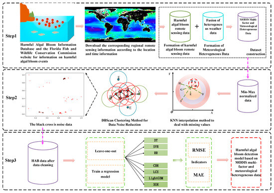
Figure 1.
General flowchart of the harmful algal bloom detection model. Step 1: Collect harmful algal bloom occurrences worldwide and obtain the corresponding remote sensing data and meteorological data with specific time and location information. Step 2: Handle missing data using the K- nearest neighbors (KNN) algorithm and perform data cleaning using the DBScan clustering method (The red dots are normal data and the black crosses are deleted noise.). Step 3: Evaluate the regression model using the processed dataset from Step 2.
2. Materials and Methods
2.1. Study Area
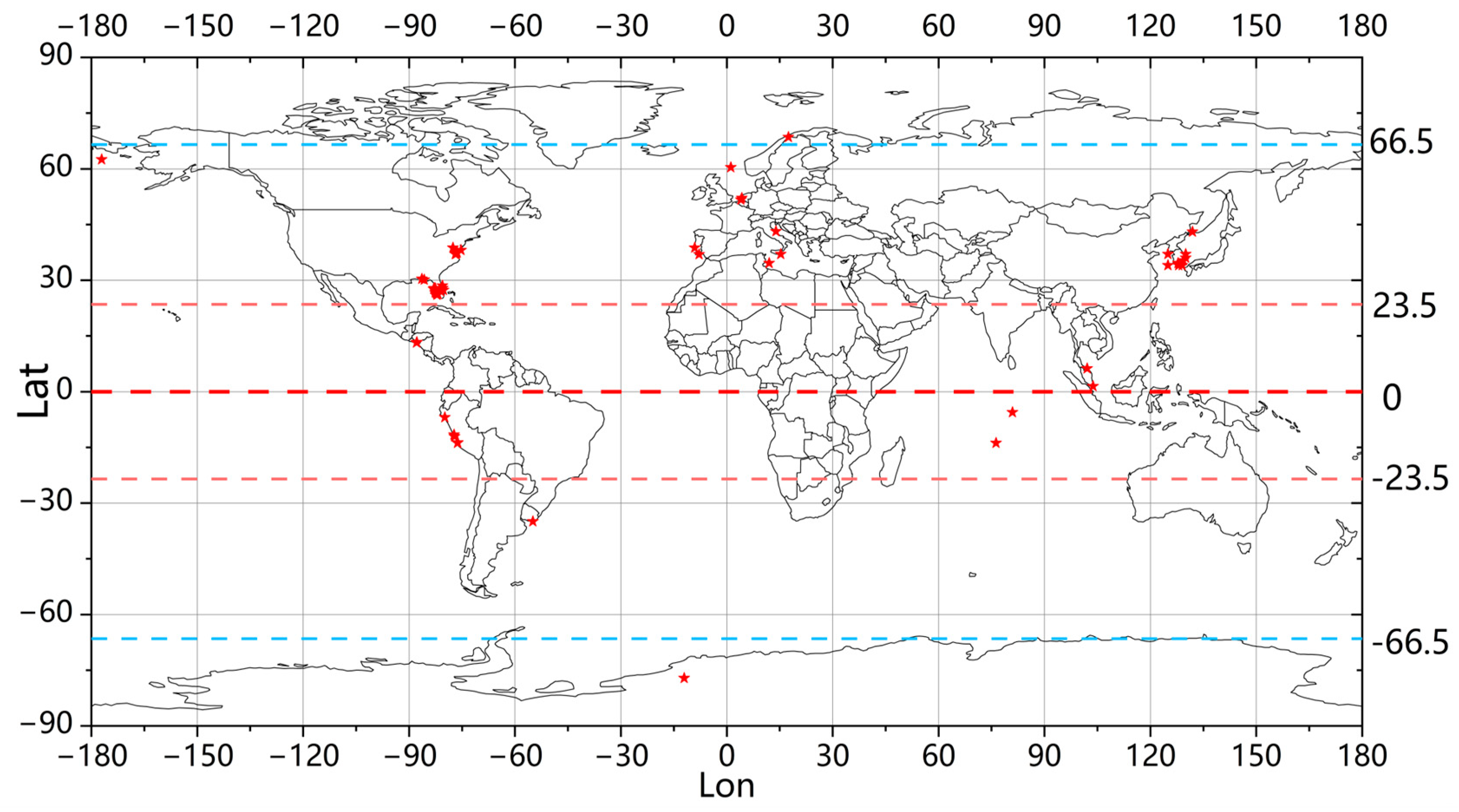
This study collected data on a total of 192 harmful algal bloom events from around the world over the past 20 years (as shown in Figure 2), thereby illustrating the global distribution of HAB occurrences.
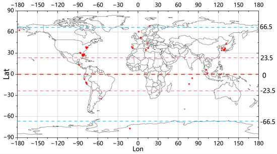
Figure 2.
The distribution of the harmful algal bloom occurrences worldwide that were collected. The areas where HABs occurred are represented by red markers.
2.2. Data Collection
The harmful algal bloom event data collected for the MODIS_MI_HABs dataset in this study are sourced from the Harmful Algal Event Database, which was established under the auspices of the National Oceanic and Atmospheric Administration (NOAA) of the United States Government. This database can be accessed at http://haedat.iode.org/browseEvents.php; (accessed on 1 May 2023). Additionally, further data were obtained from the National Office for Harmful Algal Blooms at Woods Hole Oceanographic Institution (https://hab.whoi.edu/regions-resources/national-and-international/, (accessed on 1 May 2023)) and the Florida Fish and Wildlife Conservation Commission (https://myfwc.com/, (accessed on 1 May 2023)). By amalgamating information from the aforementioned websites, harmful algal bloom data spanning the past two decades were downloaded. The data we collected comprise five major categories: spatial data, temporal data, heterogeneous meteorological information data, remote sensing data, and label data (cell concentration). The specific distribution of the MODIS_MI_HABs data are shown in Table 1.

Table 1.
All data on harmful algal bloom events.
2.3. Remote Sensing Data
2.3.1. Remote Sensing Data Acquisition
In this study, remote sensing data were obtained using the Moderate Resolution Imaging Spectroradiometer (MODIS) ocean-color satellite component, which was developed jointly by the National Aeronautics and Space Administration (NASA) and the National Oceanic and Atmospheric Administration (NOAA). This satellite measures global ocean color and temperature, among other parameters, on a global scale. The remote sensing data were acquired based on the latitude and longitude information, as well as the time information, or the collected harmful algal bloom events described in Section 2.2. First, the corresponding region (ROI) was selected based on the latitude, longitude, and time information that was obtained through NASA’s Ocean Color website (https://oceancolor.gsfc.nasa.gov/, (accessed on 20 May 2023)); the level 2 data in Aqua mode were specifically selected. Second, the data were processed through SeaWiFS Data Analysis System (SeaDAS), a software system developed by NOAA for ocean-color remote-sensing data processing, as well as analysis (https://seadas.gsfc.nasa.gov/, (accessed on 20 May 2023)).
2.3.2. Remote-Sensing Data Variables
- Chlorophyll-a
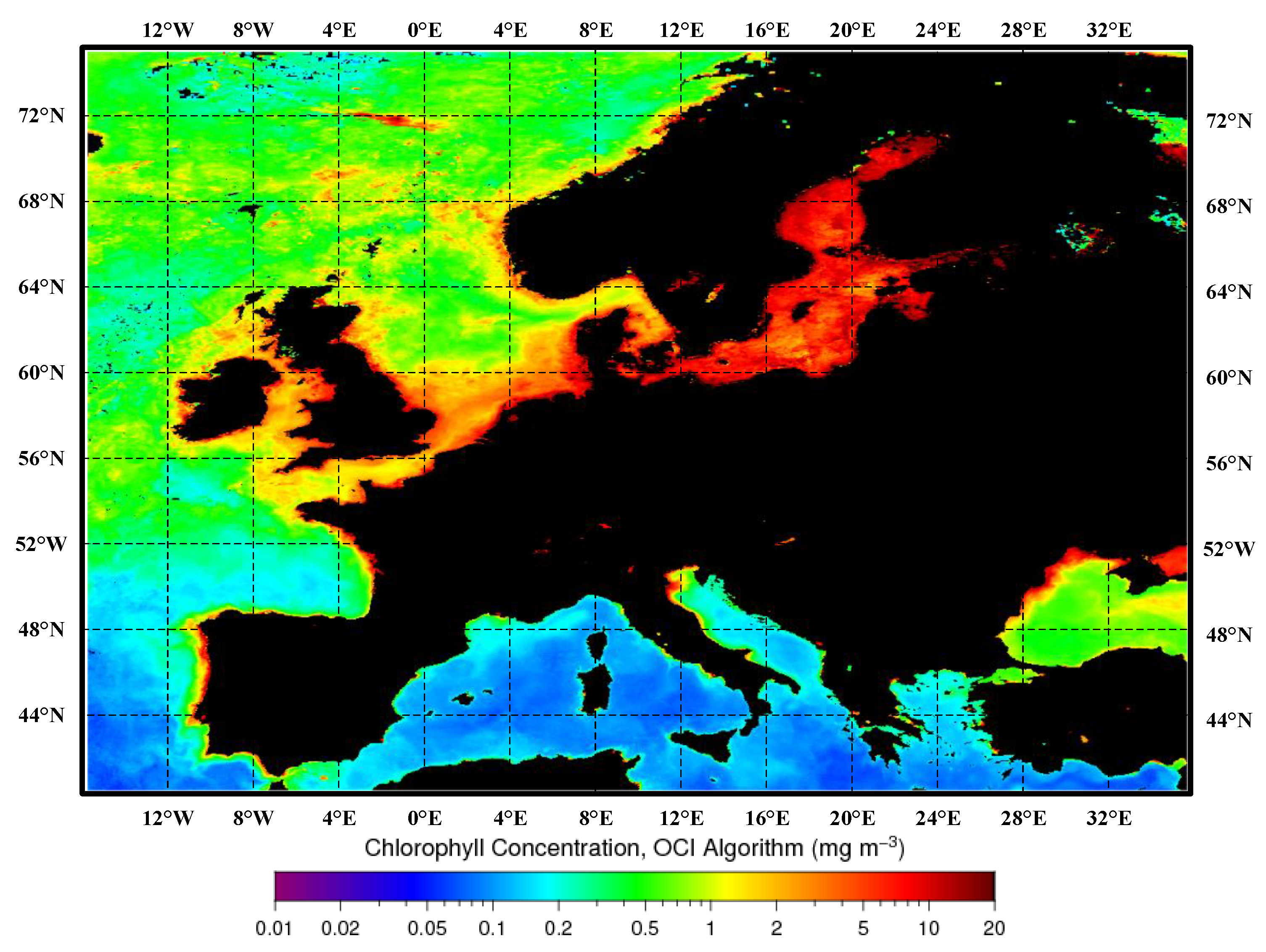
In studies on the detection of harmful algal blooms, three common pigments are often considered: chlorophyll-a, chlorophyll-b, and chlorophyll-c. Among them, chlorophyll-a has been proven to be the most representative factor associated with HABs in aquatic environments [37]. There is a strong correlation between the concentration of chlorophyll-a and the cell density of harmful algae [38]. In general, existing studies have confirmed a significant correlation between the distribution of HABs and the concentration of chlorophyll-a [39]. The monthly synthesized maps of sea-surface chlorophyll-a concentration retrieved for the Mediterranean Sea, Black Sea, and European region are illustrated in Figure 3.
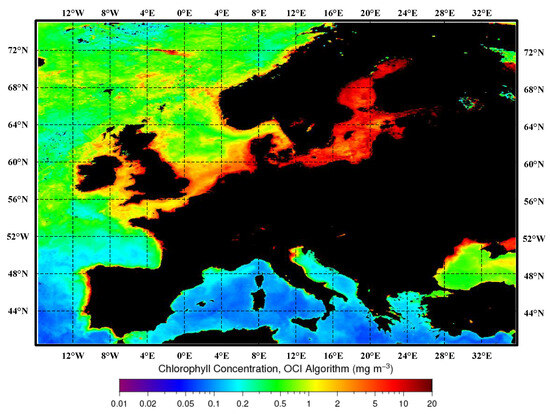
Figure 3.
Monthly composite maps of the sea-surface chlorophyll-a concentration retrieved for the Mediterranean Sea, Black Sea, and European region. In these maps, darker shades of red indicate higher chlorophyll-a concentrations, while darker shades of blue indicate lower chlorophyll-a concentrations. Black represents land.
- 2.
- Sea Surface Temperature (SST)
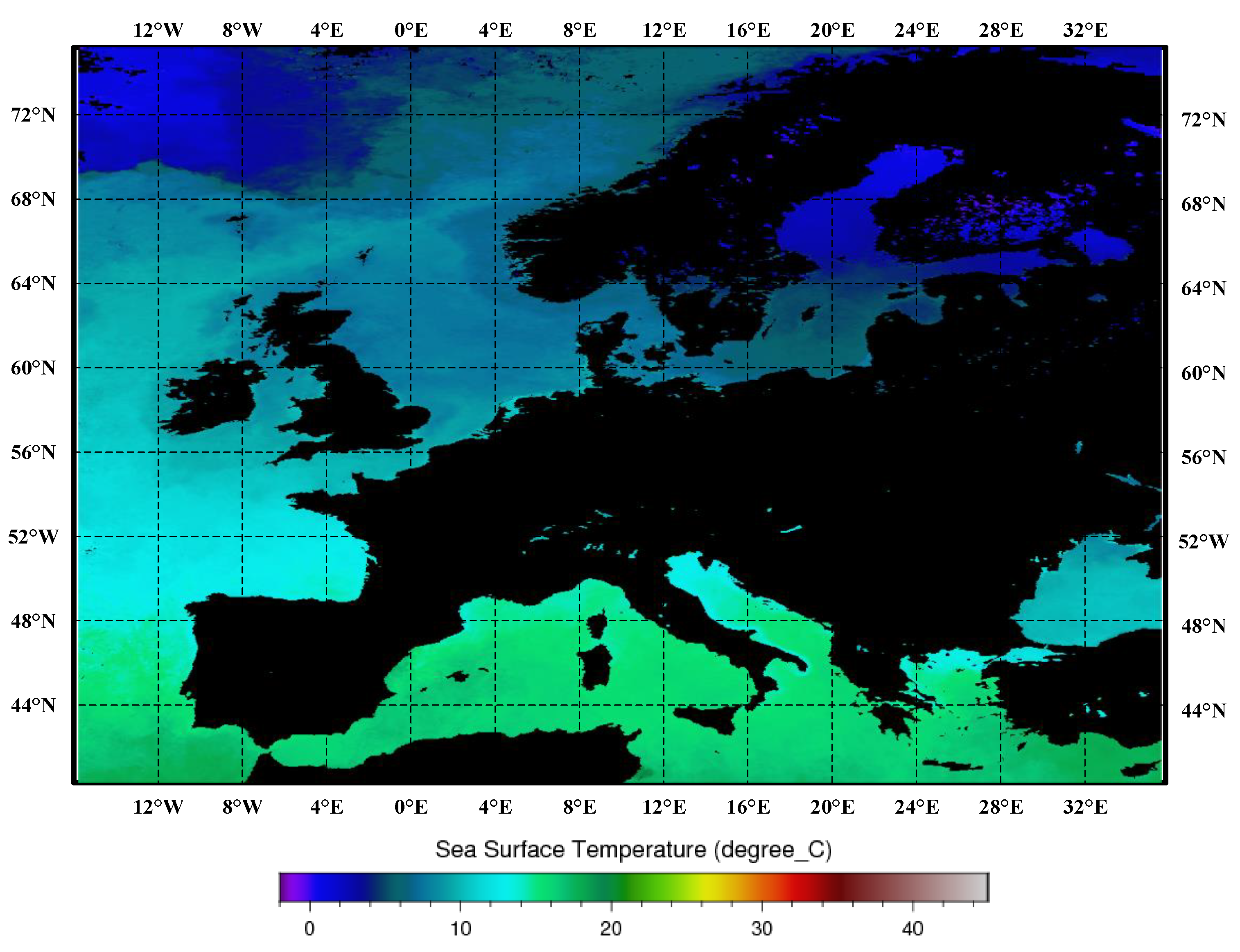
The proliferation capacity of harmful algal blooms is directly linked to sea surface temperature (SST). Temperature exerts control over the viability and ecological demands of harmful algal blooms, and this association has been substantiated in prior investigations [40,41]. The monthly synthesized maps of sea surface temperature for the Mediterranean Sea, Black Sea, and European region are presented in Figure 4.

Figure 4.
Monthly composite maps of the sea surface temperatures, as synthesized for the Mediterranean Sea, Black Sea, and European region. In these maps, darker shades of red indicate higher sea surface temperatures, while darker shades of blue indicate lower sea surface temperatures. Black represents land.
- 3.
- Photosynthetically active radiation
Photosynthetically active radiation (PAR) refers to the range of radiation utilized by harmful algae in the photosynthesis process, and it is a key factor in the proliferation of harmful algal blooms [42].
- 4.
- Relative Radiometric Stability Difference
Relative Radiometric Stability Difference (RRSDIFF) is a quality-control parameter in MODIS data. Due to variations in observational conditions, data from the same region at different times may exhibit differences. RRSDIFF is calculated to evaluate the radiometric stability difference in data from different time periods within the same region, thus ensuring data accuracy [43].
- 5.
- Seawater absorption coefficient
The seawater absorption coefficient refers to the ability of seawater to absorb light. It provides valuable information about seawater in the study of harmful algal blooms [44]. The proliferation of harmful algal blooms can impact the concentrations of dissolved organic matter and particulate matter in seawater, which, in turn, affects the seawater absorption coefficient [45,46]. In this study, six specific bands, as shown in Table 2, were used to determine the seawater absorption coefficient.
Table 2.
Seawater absorption coefficients of the six wavelength bands.
- 6.
- Backscatter coefficient
Backscattering coefficients can describe the intensity of light scattered in a backward direction. In the study of harmful algal blooms, backscattering coefficients are used to analyze the concentration of suspended particles in the water [47]. In water bodies where harmful algal blooms are present, the presence of suspended particles accelerates the proliferation of harmful algae [48]. This study utilizes two backscattering coefficients and one depolarization ratio, as shown in Table 3.
Table 3.
Scattering coefficients.
- 7.
- Angstrom Index (Angstrom)
The Angstrom exponent is an indicator that measures the impact of atmospheric scattering and absorption on light by comparing visible light signals at different wavelengths. In MODIS remote sensing data, the Angstrom exponent is used to describe particle concentrations and color variations on the surfaces of water bodies. In harmful algal bloom monitoring, color changes reflected by the Angstrom exponent can indicate variations in water quality and aid in identifying algal species. This parameter plays a crucial role in the detection of harmful algal blooms by assisting in tasks related to color changes and species identification [49].
2.3.3. Heterogeneous Weather Data
The meteorological data used in this research are the meteorological data shared by weather stations distributed all over the world. These data are the information on global meteorological conditions that are collected by members in various countries under the auspices of the World Meteorological Organization (WMO). Moreover, the information is openly shared with relevant researchers around the world for free. The data used in this paper are obtained from the National Environmental Information Website (https://www.ncei.noaa.gov/, (accessed on 20 May 2023)), which was established by the National Oceanic and Atmospheric Administration (NOAA). The distribution of global meteorological stations is illustrated in Figure 5.
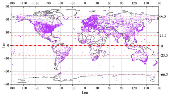
Figure 5.
Distribution of weather stations around the world. The purple dots represent weather stations. The denser the distribution of purple dots, the more weather stations in the area.
From among these data, this paper collects six kinds of heterogeneous meteorological data, as well as relative time data for the prediction of harmful algal blooms, as shown in Table 4.
Table 4.
Heterogeneous meteorological data.
2.3.4. Data Label
Harmful algal bloom cell concentration () was used as the target variable. When harmful algal blooms occurred within parameters in the data collection process, the baseline selected the harmful algal bloom events that were greater than 1,000,000 . Where the cell concentration exceeds 1,000,000 , the water discoloration indicates the occurrence of a severe harmful algal bloom. In cases of severe HABs, chlorophyll-a levels can be used to detect HABs in satellite data [50,51].
2.4. Data Cleaning
2.4.1. Missing Value Filling
Remote sensing data have the advantages of strong real-time performance, wide coverage, and high efficiency, and they are widely used in tasks monitoring the marine environment [52]. However, due to uncertain factors—such as cloud cover, complex surface features, and sensor damage—missing data have become a common phenomenon in remote sensing data [53,54]. In this study, the K- nearest neighbors interpolation (KNN) was used to fill in the missing values in the data [55,56]. Interpolating data via the KNN algorithm involves measuring distances (typically using the Euclidean distance) to identify samples within the dataset that occupy similar spaces. Subsequently, a feature-weighted average of these identified samples is computed to estimate the data value for the missing point. The missing value calculation incorporates the reciprocal of the distances as weights throughout this process. The closer the sample point is, the greater the weight is; likewise, the farther the sample point is, the smaller the weight is.
The KNN interpolation method, due to its distance-based approach for filling missing values, demonstrates wide applicability in spatially intensive remote sensing data [57,58]. On the other hand, KNN interpolation does not require a complex fitting of data or assumptions about data distribution, and thus offers high flexibility. It is suitable for various types of remote sensing data, including irregular shapes or high-dimensional datasets [59].
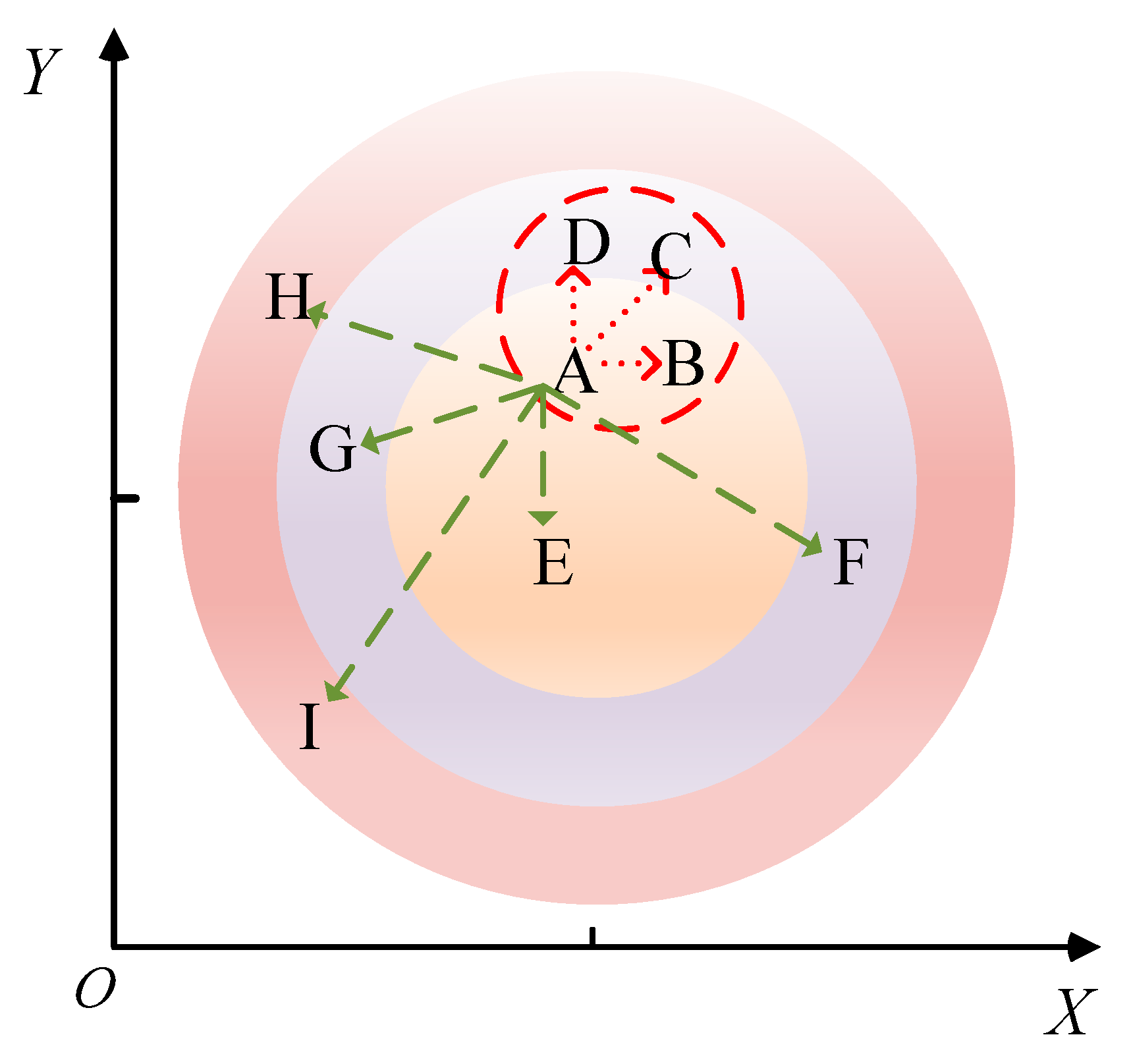
A schematic diagram illustrating the principle of the KNN missing-data handling method is depicted in Figure 6. The Euclidean distance formula is as follows:
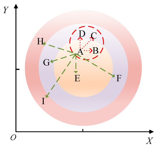
Figure 6.
The KNN missing-data processing method. In the figure, A is the data-missing point, B to I are the adjacent data samples around A, and the green dashed line and the red dashed line are the distances from the surrounding adjacent sample points to point A. Among them, the three sample points indicated by the red dotted line are the closest to the missing value point, that is, the adjacent sample points with the largest weight.
In the formula, represents the distance between sample and , represents the number of attributes, and and represent the values of and on the th attribute, respectively.
The weight formula is as follows:
In the formula, represents the weight of the th adjacent value, and represents the distance between the th adjacent value and the unknown sample.
The interpolation formula is as follows:
In the formula, represents the predicted value of the missing value sample, represents the real value of the th adjacent value, and represents the weight of the th adjacent value.
2.4.2. Data Noise Reduction
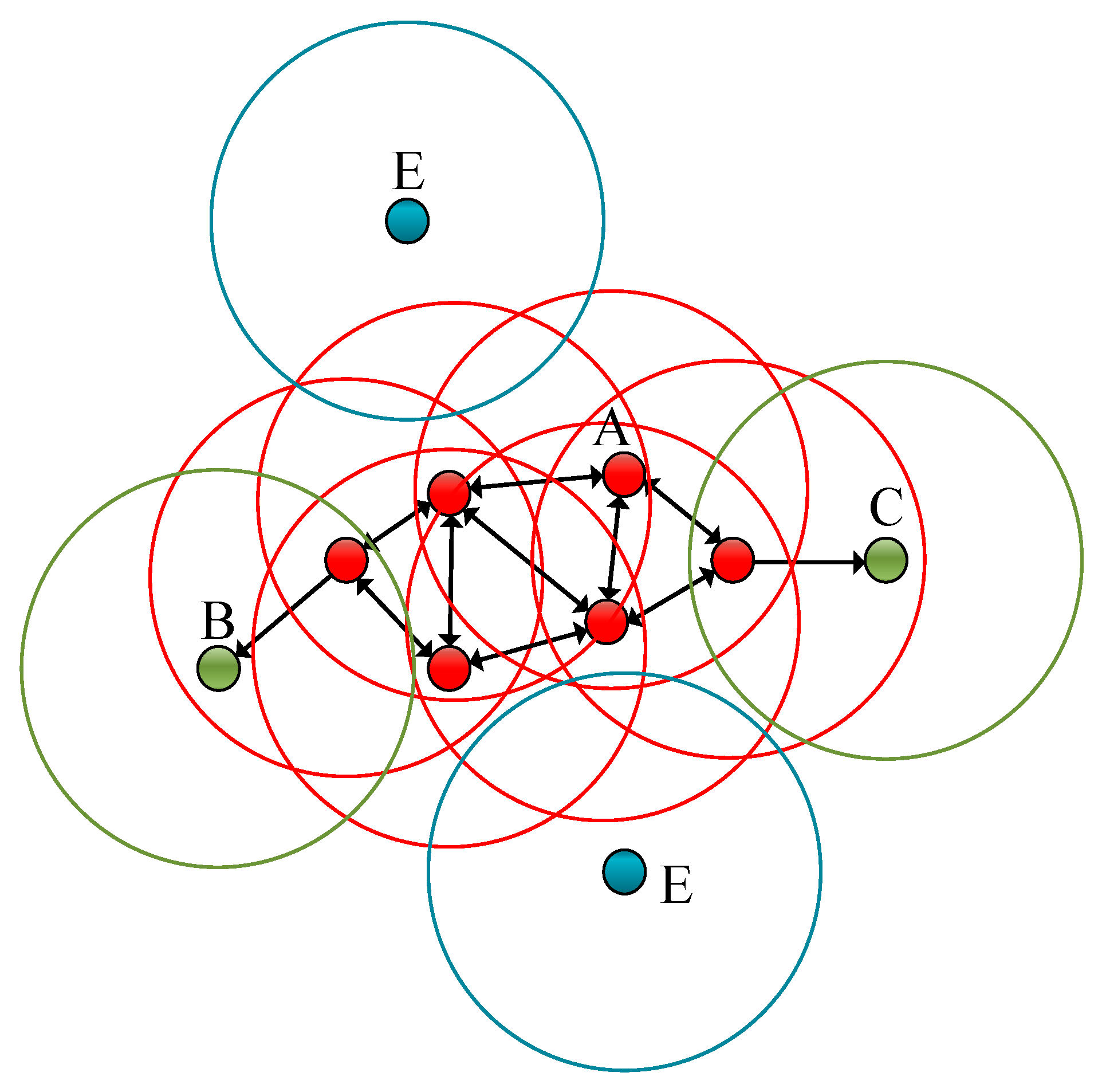
In order to ensure the quality of the data, this study uses the DBScan clustering method for data cleaning [60]. DBScan is a density-based clustering algorithm that clusters data points according to the distribution of density during dataset processing; at the same time, it also identifies initial noise points or outliers. The noise reduction principle of the DBScan clustering method is depicted in Figure 7.
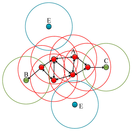
Figure 7.
The noise reduction principle of the DBScan clustering method. The red points designated as A in the figure are called the core points. (DBScan has two parameters: Epsilon—the neighborhood size, and MinPts—the minimum number of samples. If the number of points in the neighborhood is greater than or equal to the minimum number of samples, the point is among the core points, and core points can hen be associated with each other. Even where a point can be reached by the core point, if there are less than the minimum number of samples in the neighborhood, then the point is a non-core point, which is also called a boundary point. If a point is not a core point, and there are no core points within the neighborhood of the point, then they are marked as noise points.) B and C designate the green points as the boundary points, and the blue point represented by E is the noise point.
2.5. Regression Model
2.5.1. Decision Tree Regression (DT)
Decision tree regression (DT) is a non-parametric regression method based on a decision tree. This regression method establishes a decision tree model by recursively dividing sample features to achieve the target prediction [61].
2.5.2. Support Vector Machine Regression (SVR)
Support vector regression (SVR) is a regression method based on the support vector machine (SVM) [62]. SVR will try to find the best fitting hyperplane (regression line) during the training process; this method is used to achieve the purpose of regression. The main advantage of SVR is that it can perform nonlinear regression on complex data, and it has a strong generalization ability.
2.5.3. Ridge Regression (RR)
Ridge regression (RR) is a linear model commonly used in regression analysis tasks [63]. When optimizing the objective function of ridge regression, the sum of squares of the coefficients is restricted so that the variance of the model is reduced to obtain a better and more stable model.
2.5.4. Categorical Boosting (CATboost)
Categorical boosting (CATboost) is a machine learning framework based on symmetric decision trees [64]. GBR has a faster training speed, higher prediction accuracy, and there is no need for tedious feature engineering; in addition, it has stronger generalization ability and robustness.
2.5.5. Lightweight Composite Ensemble (LCE)
Lightweight composite ensemble (LCE) is a new ensemble method combining the random forest and XGboost approaches [65], and the prediction ability of the model is strengthened by this combination. Compared with the former two, it has a faster training speed, fewer hyperparameters, higher accuracy, and better performance and robustness.
2.5.6. Light Gradient Boosting Machine (LightGBM)
The light gradient boosting machine (LightGBM) is a high-performance gradient boosting algorithm based on decision trees [66]. The LightGBM uses a histogram-based algorithm for feature discretization, which improves the training efficiency and prediction speed of the algorithm to a certain extent, and it is widely used in data processing.
2.5.7. Extreme Gradient Boosting (XGR)
Extreme gradient boosting (XGBoost) is an implementation of the gradient descent (GBDT) algorithm [67]. Compared with the structure function of the traditional GBDT algorithm, XGBoost combines the second-order Taylor expansion and the regular term to correct the defect in which the tree model is easy to overfit. Furthermore, it has the advantages of faster calculation and a higher precision in the integrated model.
2.6. Experiment Details
2.6.1. Experimental Environment
The experimental environment is shown in Table 5.
Table 5.
Experimental environment configuration.
2.6.2. Model Parameter Settings
In this experiment, the optimal configuration of parameters in each model was finally determined through the parameters, as shown in Table 6.
Table 6.
Model parameter settings.
2.7. Model Evaluation Metrics
In this experiment, in order to reduce the influence of data factors on the model, the root mean square error (), mean absolute error (), coefficient of determination (), and explained variance score () were the most commonly used evaluation indicators in the regression models. However, due to the division method of leave-one-out cross-validation, only one sample was used as the test set each time, thereby resulting in an = —which makes the coefficient of determination impossible to calculate. Therefore, this paper uses the and for evaluation when using leave-one-out cross-validation.
3. Results
3.1. Evaluation and Comparison of the Seven Regression Models
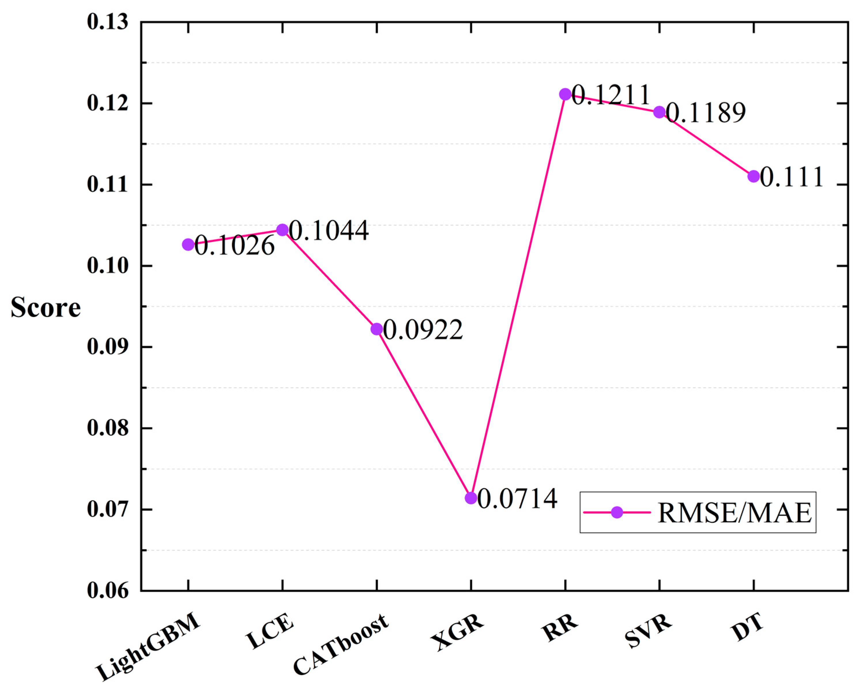
The experiment was conducted using the inversion data of oceanic information that were collected from the Ocean Color website (https://oceancolor.gsfc.nasa.gov/, (accessed on 20 May 2023)). Seven machine learning regression models (LCE, CATboost, XGR, LightGBM, RR, SVR, and DT) were employed, and leave-one-out cross-validation was performed [68,69] (with each tuple in the test set having a count of 1). Figure 8 illustrates the scores of each model based on the evaluation metrics (/). From the figure, it can be observed that among the seven machine learning regression models, the XGR model achieved the lowest scores for and (0.0714), thus indicating the best fitting performance for cell concentration in the dataset collected in this study. Additionally, the CATboost (0.0922), LightGBM (0.1026), and LCE (0.1044) models demonstrated better fitting performance compared to the other models, with minimal differences among the three. The scores of the other three regression models were higher than those of the first four models.

Figure 8.
RMSE/MAE scores when training the seven regression models using the leave-one-out cross-validation method.
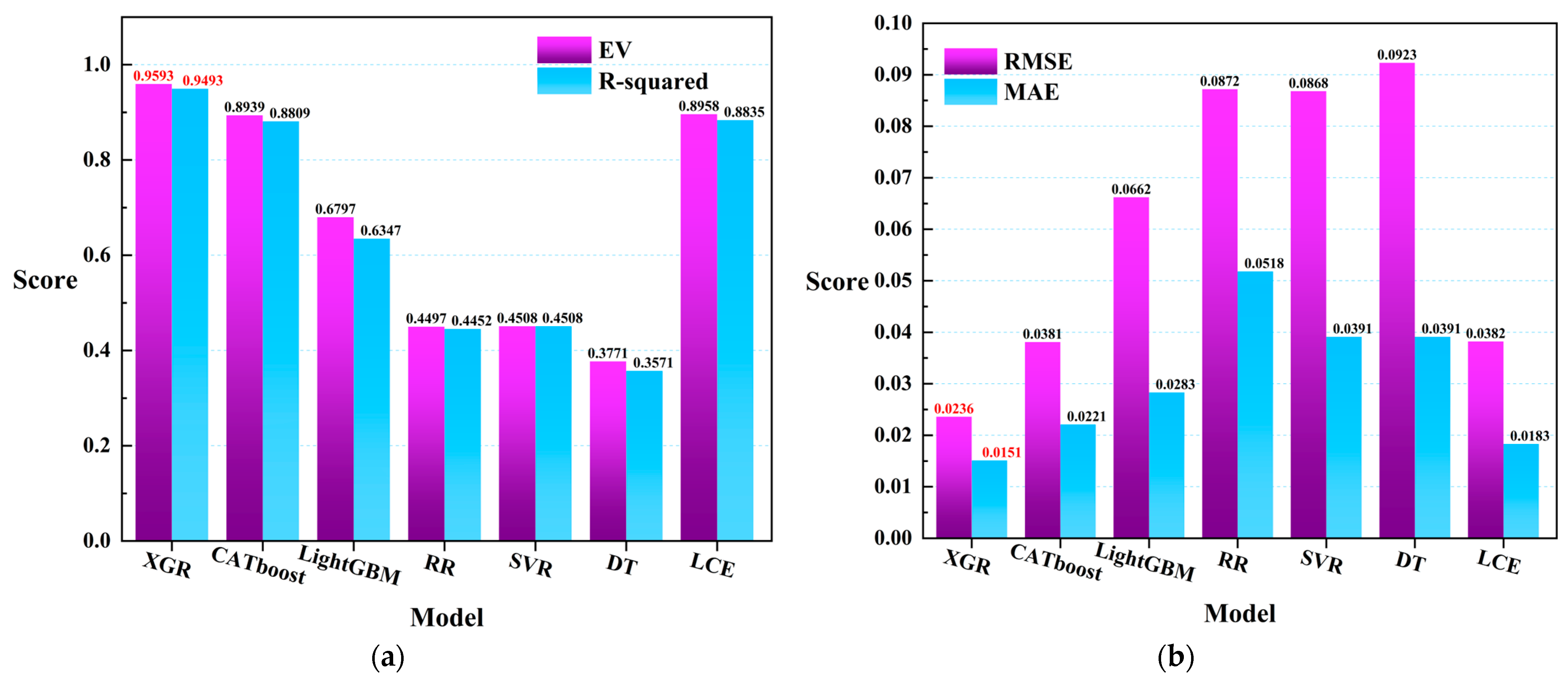
In order to further explore the relationship between meteorological data and remote sensing data in the prediction of harmful algal blooms (HABs), as well as to investigate the model performance, all samples were used to train the seven regression models in the experiment. The coefficient of determination (R-squared) and (explained variance score) were introduced as the evaluation metrics for the models, as shown in Figure 9. The results indicate that, based on the R-squared evaluation, the XGR (0.9493), CATboost (0.8809), LightGBM (0.6347), and LCE (0.8835) models achieved higher scores compared to the other models. Under the evaluation metric of the explained variance score, the performance scores for the different models were as follows: XGR (0.9593), CATboost (0.8939), LightGBM (0.6797), and LCE (0.8958). Furthermore, based on the / evaluation metrics, the XGR (0.0236/0.0151), CATboost (0.0381/0.0221), LightGBM (0.0662/0.0283), and LCE (0.0382/0.0183) models exhibited better fitting performance compared to the other models. In Figure 9, the red labels in Figure 9a represent the XGR model, which exhibited the best performance in both the explained variance () and the R-squared evaluation metrics. In Figure 9b, the red labels again denote the XGR model, which displays the optimal performance in both the root mean square error () and the mean absolute error () evaluation metrics. Based on this analysis, the XGR model demonstrated excellent performance across all of the four evaluation metrics.
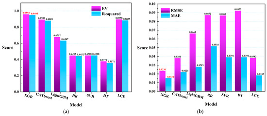
Figure 9.
(a) The R-squared and scores of the seven regression models that were trained on all of the data. (b) The and scores.
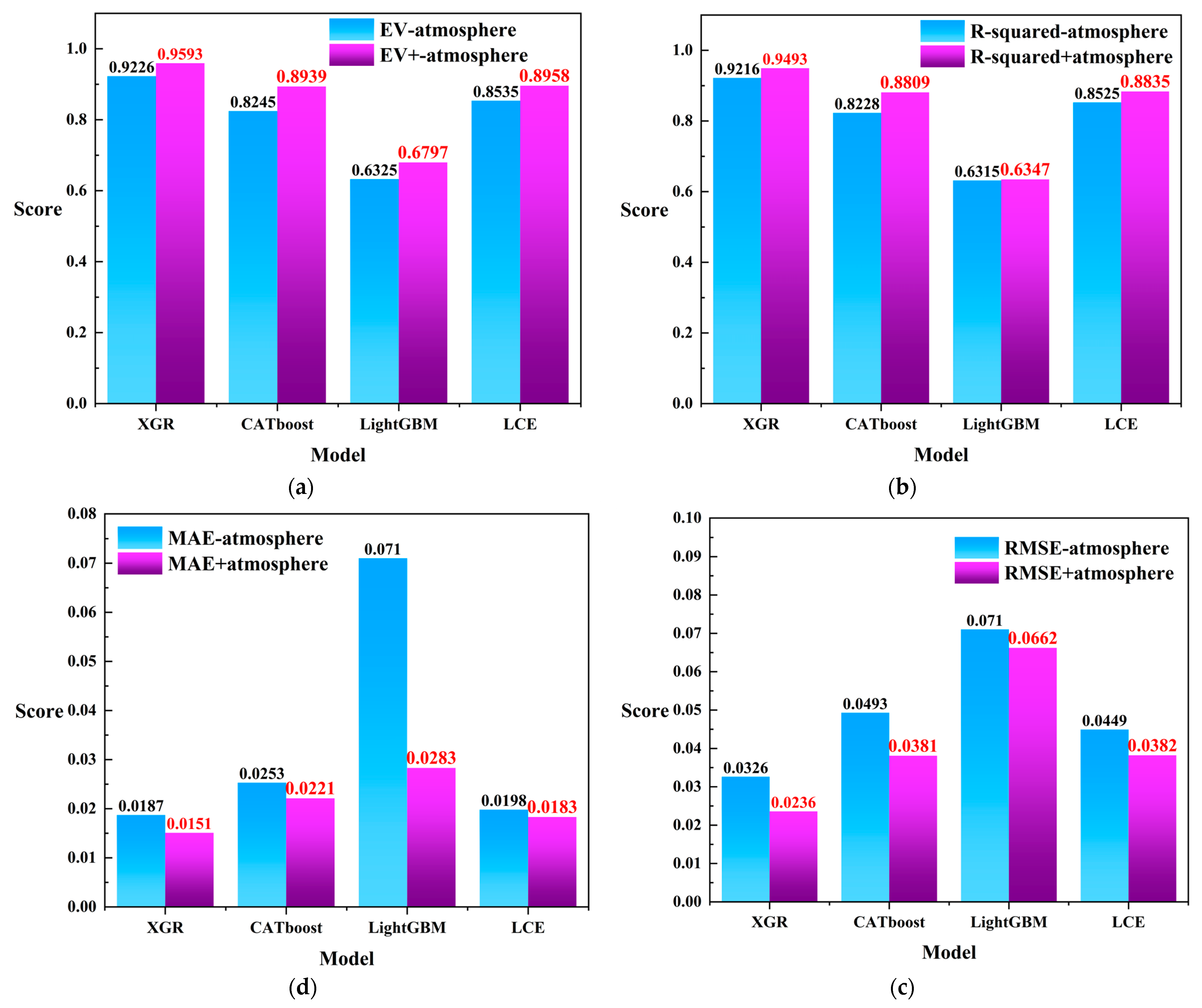
Based on the aforementioned discussion, we observed that XGR, CATboost, LightGBM, and LCE performed well in harmful algal bloom detection. In order to further validate the significance of the heterogeneous meteorological data in harmful algal bloom monitoring tasks, as well as to avoid the limitations of relying solely on remote sensing data that have been obtained by previous researchers, we conducted additional experiments by excluding the heterogeneous meteorological data and solely using the remote sensing data with the four regression models instead. The comparison of the four evaluation metrics is depicted in Figure 10. As shown in Figure 10a, the integration of the heterogeneous meteorological information in the evaluation metrics improved the performance of all four models. In Figure 10b, the incorporation of heterogeneous meteorological data enhanced the models’ performance in the R-squared evaluation metric. Similarly, in Figure 10c,d, the method of fusing meteorological heterogeneous information with remote sensing data yielded lower score tolerances than did using remote sensing data alone for both the and evaluation metrics. Furthermore, considering the combined results from Figure 10a–d, we observed that the XGR model also exhibited a favorable performance in harmful algal bloom detection tasks when using only remote sensing data ( = 0.9226; = 0.9216; = 0.0187; and = 0.0326).

Figure 10.
(a) The comparison scores for using only remote sensing data versus fusing the remote sensing data with the heterogeneous meteorological information under the evaluation metric . (b) The comparison scores for using only remote sensing data versus fusing the remote sensing data with the heterogeneous meteorological information under the evaluation metric . (c) The comparison scores for using only remote sensing data versus fusing the remote sensing data with the heterogeneous meteorological information under the evaluation metric . (d) The comparison scores for using only remote sensing data versus fusing the remote sensing data with the heterogeneous meteorological information under the evaluation metric . In the figure, “-atmosphere” represents the condition in which the heterogeneous meteorological information was not integrated, while “+atmosphere” indicates the condition where heterogeneous meteorological information was fused. Red labels in the graph indicate higher scores.
3.2. Feature Sorting and Analysis
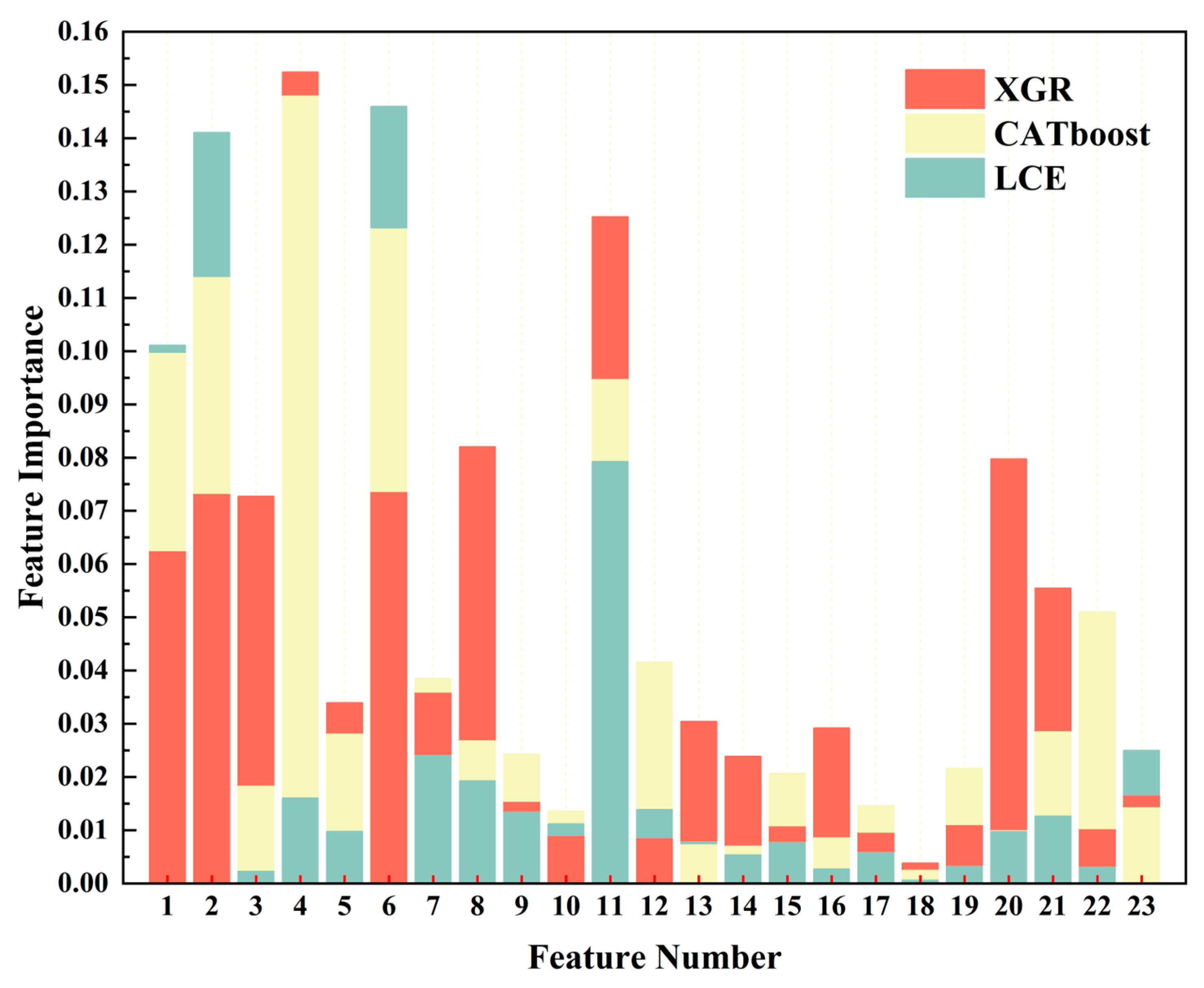
In the evaluation analysis of the seven regression models mentioned above, XGR, CATboost, and LCE demonstrated superior performances when compared to the other regression models. Therefore, in this section, we will utilize these three models to conduct a feature ranking based on their weights (the feature indices for this are listed in Appendix A Table A1). The feature rankings for the three models are illustrated in Figure 11. In the XGR model, the red section displays the feature ranking, in which the order is chlorophyll-a (0.1524), maximum sustained wind speed (0.1252), dew-point temperature (0.0820), bb_443 (0.0797), day of the year (0.0737), longitude (0.0733), sea surface temperature (0.0727), latitude (0.0626), bb_469 (0.0555), average temperature (0.0360), par (0.0339), rrsdiff (0.0304), a_547 (0.0292), a_443 (0.0238), Angstrom exponent (0.0167), sea-level pressure (0.0155), a_678 (0.0111), a_488 (0.0109), adg_443 (0.0103), a_645 (0.0097), visibility (0.0091), maximum temperature (0.0087), and a_667 (0.0038). In a tan shade in Figure 11, the CATboost model’s feature ranking was as follows: chlorophyll-a (0.1479), day of the year (0.1232), longitude (0.1140), latitude (0.0998), maximum sustained wind speed (0.0946), adg_443 (0.0510), maximum temperature (0.0416), average temperature (0.0385), bb_469 (0.0285), par (0.0280), dew-point temperature (0.0267), sea-level pressure (0.0243), a_678 (0.0216), a_488 (0.0206), sea surface temperature (0.0182), a_645 (0.0146), Angstrom exponent (0.0142), visibility (0.0136), bb_443 (0.0098), a_547 (0.0085), rrsdiff (0.0075), a_443 (0.0069), and a_667 (0.0024). In a light blue shade in Figure 11, the LCE model’s feature ranking was as follows: day of the year (0.1460), longitude (0.1410), latitude (0.1011), maximum sustained wind speed (0.0792), Angstrom exponent (0.0250), average temperature (0.0240), dew-point temperature (0.0192), chlorophyll-a (0.0160), maximum temperature (0.0138),sea-level pressure (0.0133), bb_469 (0.0126), visibility (0.0112), par (0.0097), bb_443 (0.0097), rrsdiff (0.0077), a_488 (0.0076), a_645 (0.0058), a_443 (0.0053), a_678 (0.0031), adg_443 (0.0030), a_547 (0.0027), sea surface temperature (0.0022), and a_667 (0.0006).
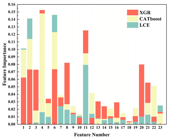
Figure 11.
Feature weight diagrams of three regression models. The red color represents XGR, the tan color represents CATboost, and the pale blue color represents LCE.
Through the analysis and explanations provided above, it became evident that, in the XGR model’s weight distribution, the five most important variables (chlorophyll-a, the maximum sustained wind speed, the dew-point temperature, bb_443, and the day of the year) included two instances of remote sensing data and two meteorological data variables. However, in the CATboost and LCE models, longitude and latitude had significant weight proportions. Furthermore, through the weight comparisons, chlorophyll-a emerged as a pivotal factor in harmful algal bloom monitoring, and it held greater weight when compared to other factors. In terms of meteorological factors, the maximum sustained wind speed also had a relatively high importance.
Through the feature analysis, we discovered that the models were sensitive to geographical characteristics, meteorological factors, and some of the remote sensing data, thus indicating variations in the harmful algal bloom characteristics across different regions. The feature weights among the three regression models were relatively evenly distributed. The difference between the highest weight, chlorophyll-a (0.1524), and the lowest weight, a_667 (0.0038) for XGR, was 0.1486. For CATboost, the difference between the highest weight, chlorophyll-a (0.1479), and the lowest weight, a_667 (0.0024), was 0.1455. In the case of LCE, the difference between the highest weight, the day of the year (0.1460), and the lowest weight, a_667 (0.0006), was 0.1454. These results indicated that the differences among the three models were not substantial.
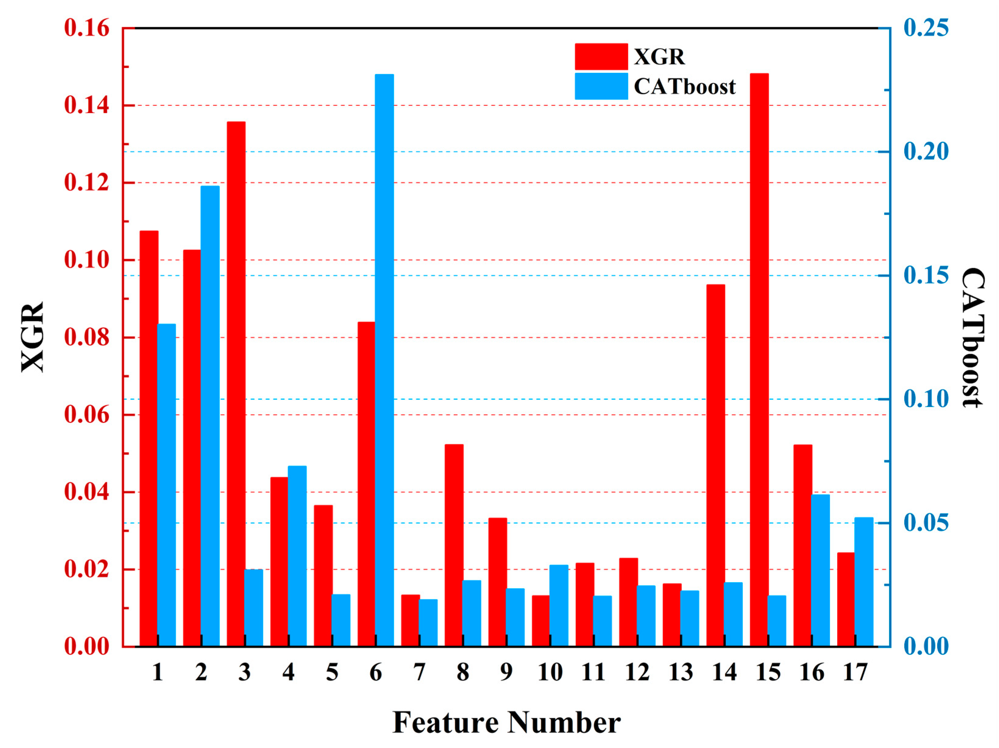
To further compare the gap between using only remote sensing data and integrating heterogeneous meteorological data, we analyzed the feature weights of the above three models when using only remote sensing data. In Figure 12, red represents the XGR model and blue represents the CATboost model. The feature weights of the XGR model when using only remote sensing data were as follows: bb_469 (0.1481), sea surface temperature (SST) (0.1357), latitude (0.1074), longitude (0.1025), bb_443 (0.0936), day of the year (0.0839), a_443 (0.0522), adg_443 (0.0521), chlorophyll-a (0.0437), par (0.0364), a_488 (0.0332), Angstrom exponent (0.0242), a_667 (0.0228), a_645 (0.0215), a_678 (0.0162), rrsdiff (0.0133), and a_547 (0.0131). For the CATboost model when using only remote sensing data, the feature weights were as follows: day of the year (0.2311), longitude (0.1860), latitude (0.1302), chlorophyll-a (0.0728), adg_443 (0.0612), Angstrom exponent (0.0521), a_547 (0.0328), SST (0.0309), a_443 (0.0266), bb_443 (0.0257), a_667 (0.0245), a_488 (0.0232), a_678 (0.0224), par (0.0209), bb_469 (0.0205), a_645 (0.0203), and rrsdiff (0.0188).
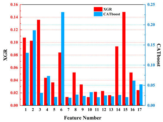
Figure 12.
The feature weight diagrams of the three regression models. The red color represents XGBoost (XGR), and the blue color represents CATboost.
When using only remote sensing data for harmful algal bloom detections, it was observed that the importance of the critical indicators like chlorophyll-a decreased after removing meteorological data. Conversely, the importance levels associated with the proportion of spatial and temporal information (longitude, latitude, and the day of the year) increased, which is not advantageous for harmful algal bloom detection tasks. However, in the XGR model, the sea surface temperature (SST) continued to play a significant role in harmful algal bloom detection, thus indirectly emphasizing the importance of heterogeneous meteorological data in these tasks.
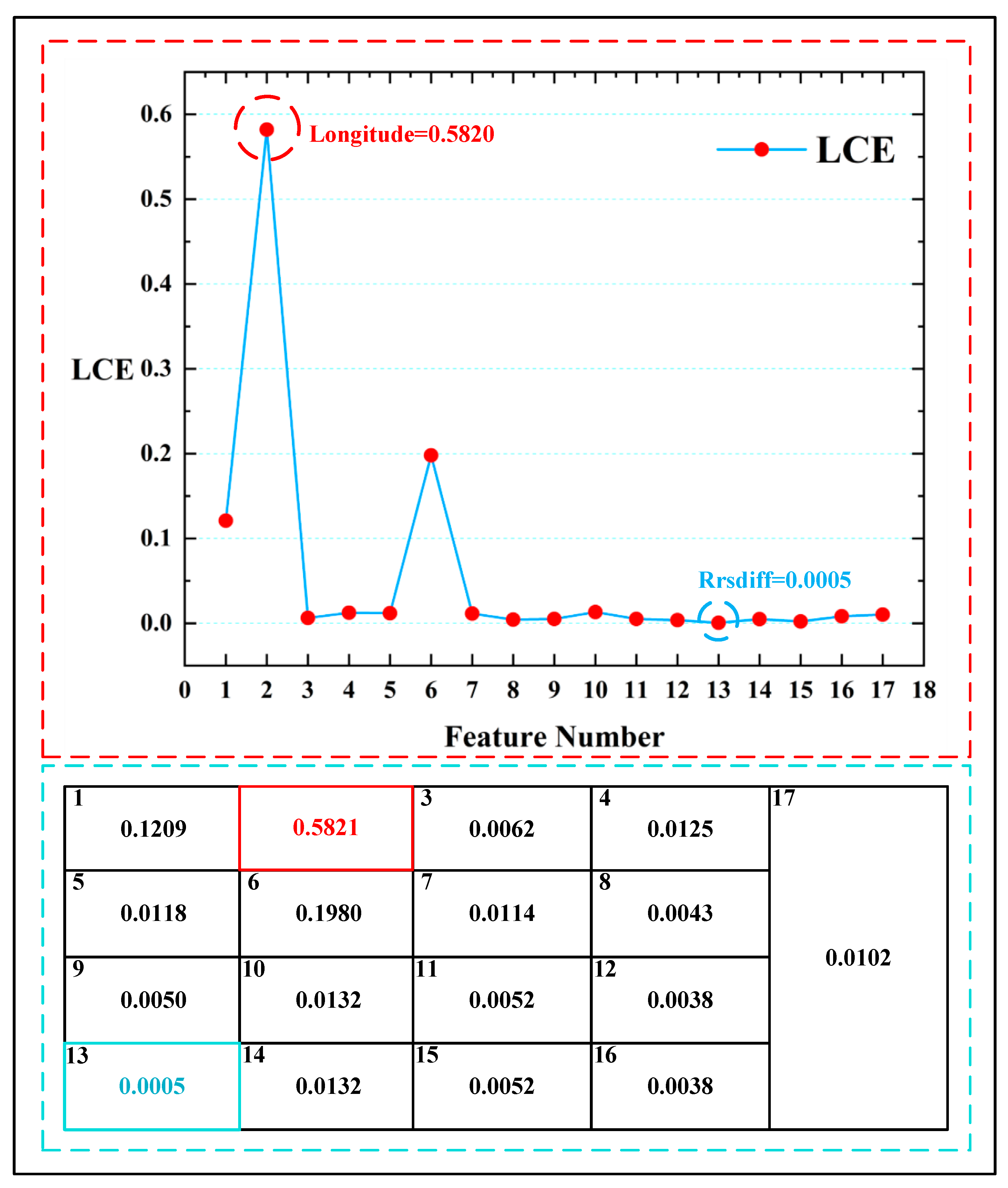
It is worth noting that, in the analysis of LCE when using only remote sensing data, the importance of spatial information (longitude) was significantly higher than other variables, with a feature weight proportion of 0.5821 for longitude. Figure 13 displays the feature weight comparison chart of the LCE model, in which the highest feature point (longitude: 0.5820) is marked by a red circle and the lowest feature point (a_678: 0.0005) is marked by a blue circle. The feature weight span of the LCE model reached 0.5815. However, such a large span in feature weights can lead to increased numerical instability, thereby affecting the regression performance of the model. From the distribution of the feature weights, it can be observed that in the context of harmful algal bloom detection when using only remote sensing data, the model’s perception of spatial information significantly increases. Due to the extensive nature of the data collection, this heightened spatial awareness could greatly influence the accuracy of harmful algal bloom detection tasks worldwide.
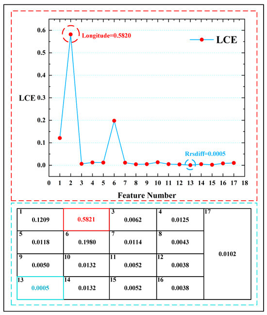
Figure 13.
The feature weight comparison chart of the LCE model. The red circle indicates the highest feature weight in the LCE variables, and the blue circle indicates the lowest feature weight in the LCE variables. The table enclosed by the blue dashed lines represents all the weight values of the LCE model.
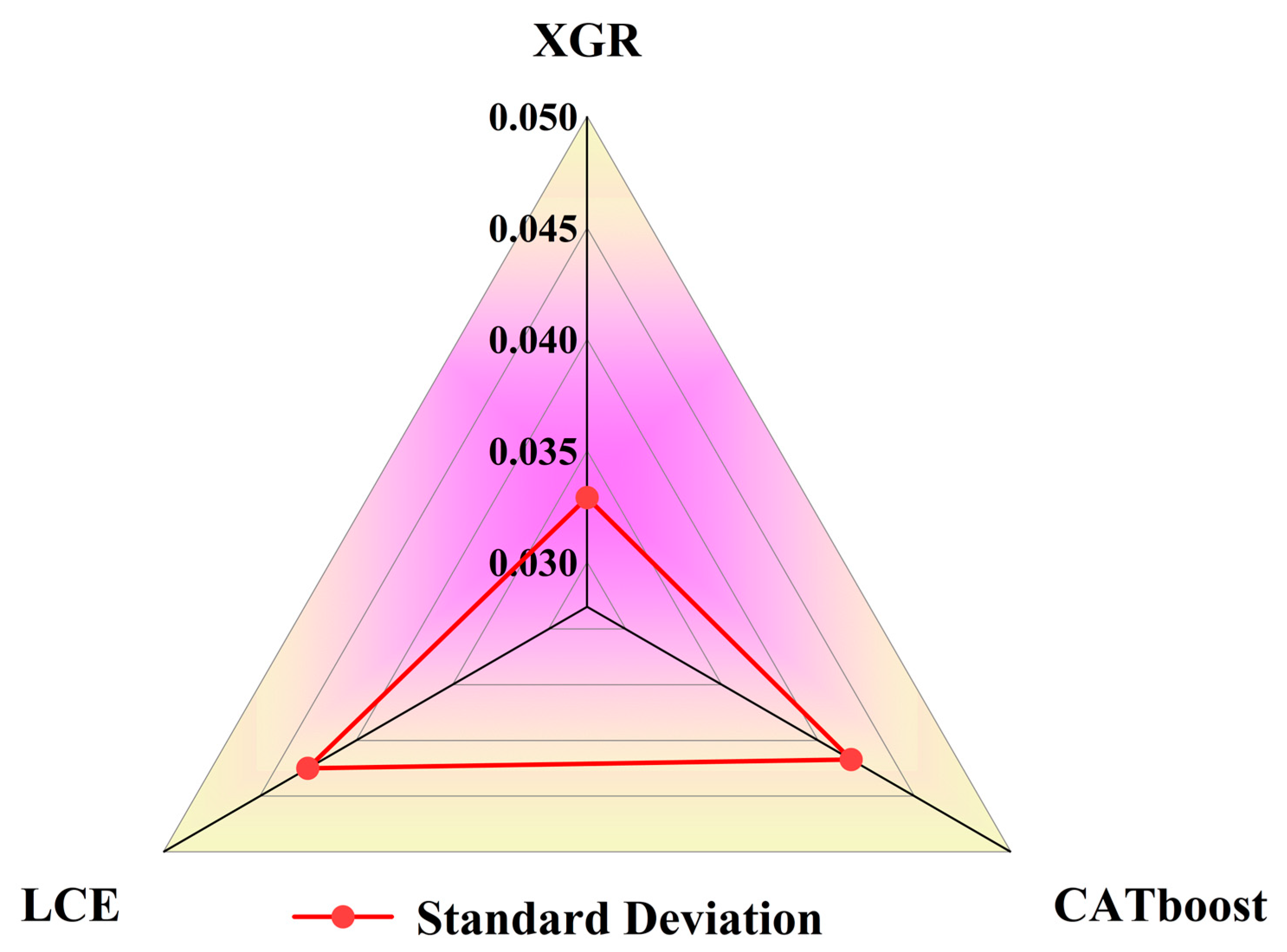
Through feature analysis, it was observed that the models were more sensitive to geographical characteristics, meteorological factors, and certain remote sensing data, thus indicating the variability of harmful algal bloom features across different regions. Among the three regression models, the feature weights were relatively evenly distributed. The difference between the highest weight, chlorophyll-a (0.1524), and the lowest weight, a_667 (0.0038), for XGR was 0.1486. For CATboost, the difference between the highest weight, chlorophyll-a (0.1479), and the lowest weight, a_667 (0.0024), was 0.1455. In the case of LCE, the difference between the highest weight, the day of the year (0.1460), and the lowest weight, a_667 (0.0006), was 0.1454. In terms of feature diversity, the standard deviations of the feature weights are compared in Figure 14 with XGR (0.0391), CATboost (0.0417), and LCE (0.0425). The results indicate that XGR and CATboost had smaller standard deviations of feature weights compared to the other models, thus making them more stable.

Figure 14.
Analysis chart of the standard deviations of feature weights of the four regression models.
Therefore, considering both the model evaluation metrics and feature analysis, XGR demonstrated a better regression performance. In this study, the XGR model was employed to achieve a regression prediction for harmful algal blooms with MODIS multifactor and heterogeneous meteorological data.
4. Discussion
The aim of this study was to develop a harmful algal bloom detection model that combines remote sensing and heterogeneous meteorological data, specifically one that is suitable for wide-ranging regions. This research primarily addresses the following: (1) the difficulty in collecting traditional marine data and its limited generalization to broader regions, and (2) the incomplete predictive factors that result from solely relying on remote sensing data. To address these issues, we integrated remote sensing and heterogeneous meteorological data to construct a harmful algal bloom detection model. This approach leverages the regional coverage and high temporal resolution of remote sensing information, while utilizing the diversity and high spatiotemporal correlation of heterogeneous meteorological data.
In response to the issues identified above, researchers have addressed the problem of low spatial resolution in MODIS images by employing super-resolution techniques that are based on deep learning algorithms. This is crucial for the precise identification and detection of harmful algal blooms within small-scale areas [70,71]. On the other hand, in the extensive monitoring of harmful algal blooms, MODIS channel data, when representing the information most responsive to regional changes in marine areas, significantly enhances the real-time monitoring of harmful algal blooms within larger regions [72].
Within the broad scope of harmful algal bloom monitoring tasks, the timely extraction of water quality information and information describing variations in sea surface color within maritime areas is challenging. This presents a significant challenge for researchers in predicting the lifecycle and spread of harmful algal blooms [73]. To enhance monitoring timeliness, researchers have adopted a data-driven approach for harmful algal bloom detection. While this method effectively utilizes water quality data during harmful algal bloom occurrences, it overlooks the crucial impact of relevant meteorological factors on harmful algal bloom incidents. Furthermore, due to the regional nature of water quality data and the uncertainty in harmful algal bloom occurrence locations, the applicability of models solely driven by water quality data is limited within extensive regions.
However, in broad-scale monitoring tasks, marine satellites exhibit exceptional performance, with wide coverage and remote sensing capabilities. This makes them ideal monitoring tools for phenomena such as harmful algal blooms [74]. The diverse channel information provided by marine satellites offers more accurate data within extensive regions, thus laying a valuable foundation for the utilization of remote sensing data and machine learning models in the broad-scale monitoring of harmful algal blooms.
To achieve this, we collected hundreds of harmful algal bloom events globally, and obtained corresponding MODIS data through ocean-color -detecting satellite instruments. We combined these data with heterogeneous meteorological information to build the MODIS_MI_HABs dataset, and we then conducted an in-depth exploration. This approach helps to overcome deficiencies in harmful algal bloom prediction. By fusing multi-band information and meteorological heterogeneous data, we harnessed the advantages of the remote sensing data. The collected harmful algal bloom dataset, combined with machine learning, provided new insights into the use of satellite remote sensing technology for harmful algal bloom detection.
To achieve an accurate detection of harmful algal blooms, this study maximized the use of remote sensing information in combination with heterogeneous meteorological data, including temperature, pressure, and wind speed. Previous research has demonstrated that climatic conditions are crucial for harmful algal bloom occurrences and spread [75,76]. However, current predictive studies often overlook meteorological factors. Furthermore, harmful algal bloom predictions that are based on ocean field data in broad regions have significant limitations. Thus, combining the extensive coverage of remote sensing in broad regions, we collected the multi-factor remote sensing data that were related to harmful algal blooms, as well as adding elaborations by means of the data collection process, to establish the MODIS_MI_HABs dataset.
To account for uncertainty-induced missing remote sensing data and to maintain data quality, we used the KNN algorithm for missing data imputations, and employed DBScan for data denoising. These steps resulted in a harmful algal bloom detection dataset that integrated remote sensing data and heterogeneous meteorological information.
In order to address issues such as missed detections, false alarms, and incomplete factor consideration in wide-ranging harmful algal bloom detection, we validated the correlation of various features with seven regression models that were based on heterogeneous harmful algal bloom data. The results indicated that regression models can effectively predict the cell concentration range of harmful algal blooms and perform predictions. The evaluation of the XGR model revealed its ability to accurately predict harmful algal bloom occurrences in broad regions. Additionally, due to limitations in the quantity of harmful algal bloom data, the XGR model exhibited performance advantages over deep learning.
Considering the limitations of fixed-area water-quality-analysis-based harmful algal bloom predictions, which face difficulties in data collection and generalization to other regions, our proposed harmful algal bloom monitoring model (which fuses remote sensing information with heterogeneous meteorological information) is timelier and more effective in wide-ranging regions. Furthermore, when compared to harmful algal bloom detection that is solely based on remote sensing information, our findings suggest that relying solely on remote sensing data yields biased results, and the stability of feature weights is also poor.
In conclusion, the XGR cell concentration prediction model based on the MODIS_MI_HABs dataset exhibited a superior performance in harmful algal bloom detection. The data collection methods proposed in this study, as well as the collected dataset, offer new research directions for scholars in the field of harmful algal bloom detection. In the future, we plan to expand the dataset further and delve deeper with harmful algal bloom information into the impacts of regional harmful algal blooms on human health. We also encourage researchers engaged in remote sensing and harmful algal bloom detection tasks to explore and extend the MODIS_MI_HABs dataset.
5. Conclusions
In this paper, we proposed a harmful algal bloom detection model that combines remote sensing and heterogeneous meteorological data. Due to the complexity of field water quality measurements in wide-ranging regions, and the limitations of solely considering remote sensing data for harmful algal bloom prediction, traditional models that are solely based on remote sensing data are prone to false alarms and missed detections. We collected hundreds of harmful algal bloom events globally and obtained corresponding MODIS data through ocean-color satellite modules, and we then combined them with heterogeneous meteorological data to construct a new dataset (MODIS_MI_HABs) for harmful algal bloom prediction. This dataset is built upon the MODIS multi-band information, and it further incorporates heterogeneous meteorological information. Simultaneously, we employed seven regression models to investigate the relationship between the data and harmful algal bloom concentration information. To assess the model’s performance, we first employed a leave-one-out cross-validation to train the data, and we used () to evaluate the model’s performance. To further validate the model, we trained it with all of the available data, introduced the coefficient of determination, and explained the variance as evaluation metrics. The results showed that, among the seven regression models, the XGBoost (XGR) model exhibited the best fitting effect. The XGR model achieved the lowest / score, of 0.0714, when using leave-one-out cross-validation, and it demonstrated a superior prediction performance when trained with all of the data ( = 0.9493, = 0.9593, = 0.0236, = 0.0151). In the feature analysis based on the regression models, the XGR model had the lowest standard deviation of feature weights (0.0391). However, the CATboost model (0.0417) showed a comparable performance. Furthermore, based on the XGR model’s feature weights, chlorophyll-a, maximum sustained wind speed, dew-point temperature, and bb_443 were the four most influential features in the harmful algal bloom detection task. In a comprehensive evaluation, the XGR model was better suited for harmful algal bloom detection when using remote sensing and heterogeneous meteorological data. We have made the MODIS_MI_HABs dataset publicly available, hoping thereby that more researchers in the field of harmful algal blooms can explore its potential. In the future, we will further collect time-series data associated with global harmful algal blooms to contribute positively to the sustainable development of marine environments.
Author Contributions
Conceptualization, Y.D.; methodology, X.B. and K.L.; formal analysis, J.L.; investigation, X.B.; resources, J.L.; data curation, X.B. and K.L.; writing—original draft preparation, X.B.; writing—review and editing, X.B.; supervision, Y.D.; funding acquisition, J.L. All authors have read and agreed to the published version of the manuscript.
Funding
This research received no external funding.
Institutional Review Board Statement
Not applicable.
Informed Consent Statement
Not applicable.
Data Availability Statement
The data used in this article can be collected and downloaded from public websites, and the specific URLs and methods are given in this article. The dataset has been publicly released and is available at https://github.com/buxiangfeng61/MODIS_MI_HABs-dataset, (accessed on 1 July 2023).
Conflicts of Interest
The authors declare no conflict of interest.
Appendix A
Table A1.
Feature numbers.
Table A1.
Feature numbers.
| Name | Parameter |
|---|---|
| 1 | Dimension |
| 2 | Longitude |
| 3 | SST |
| 4 | Chlorophyll a |
| 5 | PAR |
| 6 | Day of the year |
| 7 | Average temperature (°F) |
| 8 | Dew-point temperature (°F) |
| 9 | Sea level air pressure (HPa) |
| 10 | Visibility (mi) |
| 11 | Maximum continuous wind speed (knots) |
| 12 | Maximum temperature (°F) |
| 13 | rrsdiff |
| 14 | a_443 |
| 15 | a_488 |
| 16 | a_547 |
| 17 | a_645 |
| 18 | a_667 |
| 19 | a_678 |
| 20 | bb_443 |
| 21 | bb_469 |
| 22 | adg_443 |
| 23 | Angstrom |
References
- Chari, N.; Keerthi, S.; Sarma, N.S.; Pandi, S.R.; Chiranjeevulu, G.; Kiran, R.; Koduru, U. Fluorescence and absorption characteristics of dissolved organic matter excreted by phytoplankton species of western Bay of Bengal under axenic laboratory condition. J. Exp. Mar. Biol. Ecol. 2013, 445, 148–155. [Google Scholar] [CrossRef]
- Kahru, M.; Michell, B.G.; Diaz, A.; Miura, M. MODIS Detects a Devastating Algal Bloom in Paracas Bay, Peru. Eos Trans. AGU 2004, 85, 465–472. [Google Scholar] [CrossRef]
- Oliveira, P.B.; Moita, T.; Silva, A.; Monteiro, I.T.; Palma, A.S. Summer diatom and dinoflagellate blooms in Lisbon Bay from 2002 to 2005: Pre-conditions inferred from wind and satellite data. Prog. Oceanogr. 2009, 83, 270–277. [Google Scholar] [CrossRef]
- Tilstone, G.H.; Angel-Benavides, I.M.; Pradhan, Y.; Shutler, J.D.; Groom, S.; Sathyendranath, S. An assessment of chlorophyll-a algorithms available for SeaWiFS in coastal and open areas of the Bay of Bengal and Arabian Sea. Remote Sens. Environ. 2011, 115, 2277–2291. [Google Scholar] [CrossRef]
- Moradi, M.; Kabiri, K. Red Tide Detection in the Strait of Hormuz (East of the Persian Gulf) Using MODIS Fluorescence Data. Int. J. Remote Sens. 2012, 33, 1015–1028. [Google Scholar] [CrossRef]
- Anderson, D.M. Turning Back the Harmful Red Tide. Nature 1997, 388, 513–514. [Google Scholar] [CrossRef]
- Anderson, D.M.; Glibert, P.M.; Burkholder, J.M. Harmful Algal Blooms and Eutrophication: Nutrient Sources, Composition, and Consequences. Estuaries 2002, 25, 704–726. [Google Scholar] [CrossRef]
- Quilliam, M.A. The Role of Chromatography in the Hunt for Red Tide Toxins. J. Chromatogr. A 2003, 1000, 527–548. [Google Scholar] [CrossRef]
- Wu, H.-Y.; Zhang, F.; Dong, C.-F.; Zheng, G.-C.; Zhang, Z.-H.; Zhang, Y.-Y.; Tan, Z.-J. Variations in the Toxicity and Condition Index of Five Bivalve Species throughout a Red Tide Event Caused by Alexandrium Catenella: A Field Study. Environ. Res. 2022, 215, 114327. [Google Scholar] [CrossRef]
- Carrasco, S.; David, J. Exploratory Analysis of Toxins in Shellfish during Red Tide Harmful Algal Bloom (HABs) on the Pacific Ocean Coasts. Bachelor’s Thesis, Universidad de Investigación de Tecnología Experimental Yachay, Urcuqui, Ecuador, 2023. [Google Scholar]
- Wyrebek, R.; Fierstein, J.L.; Wells, R.G.; Machry, J.; Karjoo, S. A Case-Control Study of the Association between Karenia Brevis (Red Tide) and Biliary Atresia. medRxiv 2022. medRxiv:2022-10. [Google Scholar] [CrossRef]
- Fleming, L.E.; Kirkpatrick, B.; Backer, L.C.; Bean, J.A.; Wanner, A.; Dalpra, D.; Tamer, R.; Zaias, J.; Cheng, Y.S.; Pierce, R.; et al. Initial Evaluation of the Effects of Aerosolized Florida Red Tide Toxins (Brevetoxins) in Persons with Asthma. Environ. Health Perspect. 2005, 113, 650–657. [Google Scholar] [CrossRef]
- Kirkpatrick, B.; Fleming, L.E.; Backer, L.C.; Bean, J.A.; Tamer, R.; Kirkpatrick, G.; Kane, T.; Wanner, A.; Dalpra, D.; Reich, A.; et al. Environmental Exposures to Florida Red Tides: Effects on Emergency Room Respiratory Diagnoses Admissions. Harmful Algae 2006, 5, 526–533. [Google Scholar] [CrossRef]
- Wang, J. Prediction Model of Red Tides in Fujian Sea Area Based on BP Neural Network. J. Phys. Conf. Ser. 2020, 1486, 022001. [Google Scholar] [CrossRef]
- Chen, Y.-L.; Shen, S.-L.; Zhou, A. Assessment of Red Tide Risk by Integrating CRITIC Weight Method, TOPSIS-ASSETS Method, and Monte Carlo Simulation. Environ. Pollut. 2022, 314, 120254. [Google Scholar] [CrossRef] [PubMed]
- Qin, M.; Li, Z.; Du, Z. Red Tide Time Series Forecasting by Combining ARIMA and Deep Belief Network. Knowl. -Based Syst. 2017, 125, 39–52. [Google Scholar] [CrossRef]
- Hong-Joo, Y. Meteorological Information for Red Tide: Technical Development of Red Tide Prediction in the Korean Coastal Areas by eteorological Factors. J. Korea Inst. Inf. Commun. Eng. 2005, 9, 844–853. [Google Scholar]
- Liu, R.; Xiao, Y.; Ma, Y.; Cui, T.; An, J. Red Tide Detection Based on High Spatial Resolution Broad Band Optical Satellite Data. ISPRS J. Photogramm. Remote Sens. 2022, 184, 131–147. [Google Scholar] [CrossRef]
- Liu, R.-J.; Zhang, J.; Cui, B.-G.; Ma, Y.; Song, P.-J.; An, J.-B. Red Tide Detection Based on High Spatial Resolution Broad Band Satellite Data: A Case Study of GF-1. J. Coast. Res. 2019, 90, 120–128. [Google Scholar] [CrossRef]
- Izadi, M.; Namjoo, F.; Nikraftar, Z. A Machine Learning Approach for Harmful Algal Bloom (Red Tide) Forecasting Using MODIS Level 3 Ocean Colour Products from Google Earth Engine. In Proceedings of the AGU Fall Meeting, New Orleans, LA, USA, 13–17 December 2021; p. OS55B-0710. [Google Scholar]
- Kazmi, S.S.U.H.; Yapa, N.; Karunarathna, S.C.; Suwannarach, N. Perceived Intensification in Harmful Algal Blooms Is a Wave of Cumulative Threat to the Aquatic Ecosystems. Biology 2022, 11, 852. [Google Scholar] [CrossRef]
- Glibert, P.M.; Icarus Allen, J.; Artioli, Y.; Beusen, A.; Bouwman, L.; Harle, J.; Holmes, R.; Holt, J. Vulnerability of Coastal Ecosystems to Changes in Harmful Algal Bloom Distribution in Response to Climate Change: Projections Based on Model Analysis. Glob. Chang. Biol. 2014, 20, 3845–3858. [Google Scholar] [CrossRef]
- Pant, R.; Gupta, A.; Srivastava, S.; Singh, A.; Patrick, N. Association of Algae to Water Pollution and Waste Water Treatment. In Microbial Technology for Sustainable E-Waste Management; Debbarma, P., Kumar, S., Suyal, D.C., Soni, R., Eds.; Springer International Publishing: Cham, Switzerland, 2023; pp. 213–230. ISBN 978-3-031-25678-3. [Google Scholar]
- Vianna LF, N.; de Souza, R.V.; Schramm, M.A.; Alves, T.P. Using climate reanalysis and remote sensing-derived data to create the basis for predicting the occurrence of algal blooms, harmful algal blooms and toxic events in Santa Catarina, Brazil. Sci. Total Environ. 2023, 880, 163086. [Google Scholar] [PubMed]
- Soto, D.; León-Muñoz, J.; Garreaud, R.; Quiñones, R.A.; Morey, F. Scientific Warnings Could Help to Reduce Farmed Salmon Mortality Due to Harmful Algal Blooms. Mar. Policy 2021, 132, 104705. [Google Scholar] [CrossRef]
- Grasso, C.R.; Pokrzywinski, K.L.; Waechter, C.; Rycroft, T.; Zhang, Y.; Aligata, A.; Kramer, M.; Lamsal, A. A Review of Cyanophage–Host Relationships: Highlighting Cyanophages as a Potential Cyanobacteria Control Strategy. Toxins 2022, 14, 385. [Google Scholar] [CrossRef] [PubMed]
- Zheng, L.; Wang, H.; Liu, C.; Zhang, S.; Ding, A.; Xie, E.; Li, J.; Wang, S. Prediction of Harmful Algal Blooms in Large Water Bodies Using the Combined EFDC and LSTM Models. J. Environ. Manag. 2021, 295, 113060. [Google Scholar] [CrossRef]
- Ding, Y.; Wang, M.; Fu, Y.; Zhang, L.; Wang, X. A Wildfire Detection Algorithm Based on the Dynamic Brightness Temperature Threshold. Forests 2023, 14, 477. [Google Scholar] [CrossRef]
- Gibson, R.; Danaher, T.; Hehir, W.; Collins, L. A Remote Sensing Approach to Mapping Fire Severity in South-Eastern Australia Using Sentinel 2 and Random Forest. Remote Sens. Environ. 2020, 240, 111702. [Google Scholar] [CrossRef]
- Dong, H.; Wu, H.; Sun, P.; Ding, Y. Wildfire Prediction Model Based on Spatial and Temporal Characteristics: A Case Study of a Wildfire in Portugal’s Montesinho Natural Park. Sustainability 2022, 14, 10107. [Google Scholar] [CrossRef]
- Takahashi, W.; Kawamura, H.; Omura, T.; Furuya, K. Detecting Red Tides in the Eastern Seto Inland Sea with Satellite Ocean Color Imagery. J. Oceanogr. 2009, 65, 647–656. [Google Scholar] [CrossRef]
- Stumpf, R.P. Applications of Satellite Ocean Color Sensors for Monitoring and Predicting Harmful Algal Blooms. Hum. Ecol. Risk Assess. Int. J. 2001, 7, 1363–1368. [Google Scholar] [CrossRef]
- de Araújo Carvalho, G.; Minnett, P.; Baringer, W.; Banzon, V. Detection of Florida “red tides” from SeaWiFS and MODIS imagery. In Proceedings of the Anais XIII Simpósio Brasileiro de Sensoriamento Remoto, Floriandzpolis, Brazil, 21–26 April 2007; pp. 4581–4588. [Google Scholar]
- Hu, C.; Muller-Karger, F.E.; Taylor, C.J.; Carder, K.L.; Kelble, C.; Johns, E.; Heil, C.A. Red Tide Detection and Tracing Using MODIS Fluorescence Data: A Regional Example in SW Florida Coastal Waters. Remote Sens. Environ. 2005, 97, 311–321. [Google Scholar] [CrossRef]
- Hallegraeff, G.M. Ocean Climate Change, Phytoplankton Community Responses, and Harmful Algal Blooms: A Formidable Predictive Challenge. J. Phycol. 2010, 46, 220–235. [Google Scholar] [CrossRef]
- Bricaud, A.; Bosc, E.; Antoine, D. Algal Biomass and Sea Surface Temperature in the Mediterranean Basin: Intercomparison of Data from Various Satellite Sensors, and Implications for Primary Production Estimates. Remote Sens. Environ. 2002, 81, 163–178. [Google Scholar] [CrossRef]
- Wang, G.; Lee, Z.; Mouw, C. Multi-Spectral Remote Sensing of Phytoplankton Pigment Absorption Properties in Cyanobacteria Bloom Waters: A Regional Example in the Western Basin of Lake Erie. Remote Sens. 2017, 9, 1309. [Google Scholar] [CrossRef]
- Shang, S.L.; Dong, Q.; Hu, C.M.; Lin, G.; Li, Y.H.; Shang, S.P. On the Consistency of MODIS Chlorophyll α Products in the Northern South China Sea. Biogeosciences 2014, 11, 269–280. [Google Scholar] [CrossRef]
- Lee, S.; Lee, D. Improved Prediction of Harmful Algal Blooms in Four Major South Korea’s Rivers Using Deep Learning Models. Int. J. Environ. Res. Public Health 2018, 15, 1322. [Google Scholar] [CrossRef] [PubMed]
- Chen, C.; Liang, J.; Yang, G.; Sun, W. Spatio-temporal distribution of harmful algal blooms and their correlations with marine hydrological elements in offshore areas, China. Ocean Coastal Manag. 2023, 238, 106554. [Google Scholar] [CrossRef]
- Errera, R.M.; Yvon-Lewis, S.; Kessler, J.D.; Campbell, L. Reponses of the Dinoflagellate Karenia Brevis to Climate Change: PCO2 and Sea Surface Temperatures. Harmful Algae 2014, 37, 110–116. [Google Scholar] [CrossRef]
- Williams, G.N.; Nocera, A.C. Bio-Optical Trends of Waters around Valdés Biosphere Reserve: An Assessment of the Temporal Variability Based on 20 Years of Ocean Color Satellite Data. Mar. Environ. Res. 2023, 186, 105923. [Google Scholar] [CrossRef]
- Chander, G.; Xiong, X.J.; Choi, T.J.; Angal, A. Monitoring On-Orbit Calibration Stability of the Terra MODIS and Landsat 7 ETM+ Sensors Using Pseudo-Invariant Test Sites. Remote Sens. Environ. 2010, 114, 925–939. [Google Scholar] [CrossRef]
- Zheng, G.; Stramski, D. A Model Based on Stacked-constraints Approach for Partitioning the Light Absorption Coefficient of Seawater into Phytoplankton and Non-phytoplankton Components. J. Geophys. Res. Oceans 2013, 118, 2155–2174. [Google Scholar] [CrossRef]
- Ahn, Y.-H.; Shanmugam, P. Detecting the Red Tide Algal Blooms from Satellite Ocean Color Observations in Optically Complex Northeast-Asia Coastal Waters. Remote Sens. Environ. 2006, 103, 419–437. [Google Scholar] [CrossRef]
- Pogash, M.A. Broadband Cavity-Enhanced Spectroscopy and Photoacoustic Spectroscopy for UV-Vis Observation of Aerosol Optical Properties—ProQuest. Available online: https://www.proquest.com/openview/e0927d43a69be1ad7af12f04b909c92a/1?pq-origsite=gscholar&cbl=18750&diss=y (accessed on 14 June 2023).
- Khan, R.M.; Salehi, B.; Mahdianpari, M.; Mohammadimanesh, F.; Mountrakis, G.; Quackenbush, L.J. A Meta-Analysis on Harmful Algal Bloom (HAB) Detection and Monitoring: A Remote Sensing Perspective. Remote Sens. 2021, 13, 4347. [Google Scholar] [CrossRef]
- He, X.; Chen, J.; Wu, D.; Sun, P.; Ma, X.; Wang, J.; Liu, L.; Chen, K.; Wang, B. Distribution Characteristics and Environmental Control Factors of Lipophilic Marine Algal Toxins in Changjiang Estuary and the Adjacent East China Sea. Toxins 2019, 11, 596. [Google Scholar] [CrossRef] [PubMed]
- Smith, I. Remote Sensing and Artificial Intelligence-Based Modeling and Prediction of Harmful Algal Blooms in Lake Pontchartrain. Master’s Thesis, Louisiana State University and Agricultural and Mechanical College, Baton Rouge, LA, USA, 23 May 2023. [Google Scholar]
- Silva, E.; Counillon, F.; Brajard, J.; Pettersson, L.H.; Naustvoll, L. Forecasting harmful algae blooms: Application to Dinophysis acuminata in northern Norway. Harmful Algae 2023, 126, 102442. [Google Scholar] [CrossRef]
- Zhou, Z.; Shi, H.; Fu, Q.; Ding, Y.; Li, T.; Liu, S. Investigating the propagation from meteorological to hydrological drought by introducing the nonlinear dependence with directed information transfer index. Water Resour. Res. 2021, 57, e2021WR030028. [Google Scholar] [CrossRef]
- Katsaros, K. BOOK REVIEW—An Introduction to Ocean Remote Sensing. Oceanography 2005, 18, 86–89. [Google Scholar] [CrossRef]
- Wang, S.; Li, W.; Hou, S.; Guan, J.; Yao, J. STA-GAN: A Spatio-Temporal Attention Generative Adversarial Network for Missing Value Imputation in Satellite Data. Remote Sens. 2023, 15, 88. [Google Scholar] [CrossRef]
- King, M.D.; Platnick, S.; Menzel, W.P.; Ackerman, S.A.; Hubanks, P.A. Spatial and Temporal Distribution of Clouds Observed by MODIS Onboard the Terra and Aqua Satellites. IEEE Trans. Geosci. Remote Sens. 2013, 51, 3826–3852. [Google Scholar] [CrossRef]
- Sahoo, A.; Ghose, D.K. Imputation of Missing Precipitation Data Using KNN, SOM, RF, and FNN. Soft. Comput. 2022, 26, 5919–5936. [Google Scholar] [CrossRef]
- Armina, R.; Zain, A.M.; Ali, N.A.; Sallehuddin, R. A Review on Missing Value Estimation Using Imputation Algorithm. J. Phys. Conf. Ser. 2017, 892, 012004. [Google Scholar] [CrossRef]
- Fu, Y.; He, H.S.; Hawbaker, T.J.; Henne, P.D.; Zhu, Z.; Larsen, D.R. Evaluating k-Nearest Neighbor (k NN) Imputation Models for Species-Level Aboveground Forest Biomass Mapping in Northeast China. Remote Sens. 2019, 11, 2005. [Google Scholar] [CrossRef]
- Zhang, H.; Yao, Y.; Hu, M.; Xu, C.; Su, X.; Che, D.; Peng, W. A Tropospheric Zenith Delay Forecasting Model Based on a Long Short-Term Memory Neural Network and Its Impact on Precise Point Positioning. Remote Sens. 2022, 14, 5921. [Google Scholar] [CrossRef]
- Malambo, L.; Heatwole, C.D. A multitemporal profile-based interpolation method for gap filling nonstationary data. IEEE Trans. Geosci. Remote Sens. 2015, 54, 252–261. [Google Scholar] [CrossRef]
- Shakya, V.; Makwana, R.R.S. Feature Selection Based Intrusion Detection System Using the Combination of DBSCAN, K-Mean++ and SMO Algorithms. In Proceedings of the 2017 International Conference on Trends in Electronics and Informatics (ICEI), Tirunelveli, India, 11–12 May 2017; pp. 928–932. [Google Scholar]
- Loh, W.-Y. Classification and Regression Trees. WIREs Data Min. Knowl. Discov. 2011, 1, 14–23. [Google Scholar] [CrossRef]
- Cortes, C.; Vapnik, V. Support-Vector Networks. Mach. Learn. 1995, 20, 273–297. [Google Scholar] [CrossRef]
- Hoerl, A.E.; Kennard, R.W. Ridge Regression: Biased Estimation for Nonorthogonal Problems. Technometrics 1970, 12, 55–67. [Google Scholar] [CrossRef]
- Prokhorenkova, L.; Gusev, G.; Vorobev, A.; Dorogush, A.V.; Gulin, A. CatBoost: Unbiased boosting with categorical features. Adv. Neural Inf. Process. Syst. 2018, 31. [Google Scholar]
- Fauvel, K.; Fromont, É.; Masson, V.; Faverdin, P.; Termier, A. XEM: An Explainable-by-Design Ensemble Method for Multivariate Time Series Classification. Data Min. Knowl. Disc. 2022, 36, 917–957. [Google Scholar] [CrossRef]
- Ke, G.; Meng, Q.; Finley, T.; Wang, T.; Chen, W.; Ma, W.; Ye, Q.; Liu, T.-Y. LightGBM: A Highly Efficient Gradient Boosting Decision Tree. In Advances in Neural Information Processing Systems; Curran Associates, Inc.: Red Hook, NY, USA, 2017; Volume 30. [Google Scholar]
- Chen, T.; Guestrin, C. XGBoost: A Scalable Tree Boosting System. In Proceedings of the 22nd ACM SIGKDD International Conference on Knowledge Discovery and Data Mining, San Francisco, CA, USA, 13–17 August 2016; Available online: https://dl.acm.org/doi/abs/10.1145/2939672.2939785 (accessed on 14 June 2023).
- Wong, T.-T. Performance Evaluation of Classification Algorithms by K-Fold and Leave-One-out Cross Validation. Pattern Recognit. 2015, 48, 2839–2846. [Google Scholar] [CrossRef]
- Fukunaga, K.; Hostetler, L. The Estimation of the Gradient of a Density Function, with Applications in Pattern Recognition. IEEE Trans. Inf. Theory 1975, 21, 32–40. [Google Scholar] [CrossRef]
- Kwon, D.H.; Hong, S.M.; Abbas, A.; Park, S.; Nam, G.; Yoo, J.H.; Kim, K.; Kim, H.T.; Pyo, J.; Cho, K.H. Deep learning-based super-resolution for harmful algal bloom monitoring of inland water. GIScience Remote Sens. 2023, 60, 2249753. [Google Scholar] [CrossRef]
- Cui, B.; Zhang, H.; Jing, W.; Liu, H.; Cui, J. SRSe-net: Super-resolution-based semantic segmentation network for green tide extraction. Remote Sens. 2022, 14, 710. [Google Scholar] [CrossRef]
- Caballero, I.; Fernández, R.; Escalante, O.M.; Mamán, L.; Navarro, G. New capabilities of Sentinel-2A/B satellites combined with in situ data for monitoring small harmful algal blooms in complex coastal waters. Sci. Rep. 2020, 10, 8743. [Google Scholar] [CrossRef] [PubMed]
- Rodríguez-Benito, C.V.; Navarro, G.; Caballero, I. Using Copernicus Sentinel-2 and Sentinel-3 data to monitor harmful algal blooms in Southern Chile during the COVID-19 lockdown. Mar. Pollut. Bull. 2020, 161, 111722. [Google Scholar] [CrossRef] [PubMed]
- Seltenrich, N. Keeping tabs on HABs: New tools for detecting, monitoring, and preventing harmful algal blooms. Environ. Health Perspect. 2014, 122. [Google Scholar] [CrossRef]
- Griffith, A.W.; Gobler, C.J. Harmful Algal Blooms: A Climate Change Co-Stressor in Marine and Freshwater Ecosystems. Harmful Algae 2020, 91, 101590. [Google Scholar] [CrossRef]
- Gobler, C.J. Climate Change and Harmful Algal Blooms: Insights and Perspective. Harmful Algae 2020, 91, 101731. [Google Scholar] [CrossRef]


Disclaimer/Publisher’s Note: The statements, opinions and data contained in all publications are solely those of the individual author(s) and contributor(s) and not of MDPI and/or the editor(s). MDPI and/or the editor(s) disclaim responsibility for any injury to people or property resulting from any ideas, methods, instructions or products referred to in the content. |
© 2023 by the authors. Licensee MDPI, Basel, Switzerland. This article is an open access article distributed under the terms and conditions of the Creative Commons Attribution (CC BY) license (https://creativecommons.org/licenses/by/4.0/).