Smart Building Thermal Management: A Data-Driven Approach Based on Dynamic and Consensus Clustering

Abstract

A customized and cost-effective building thermal control system is critical for accommodating thermal performance differences within the building, as well as satisfying the individual thermal comfort needs of occupants. Moreover, incorporating a building indoor thermal simulation procedure into the thermal control system can reduce the necessity of installing various expensive sensors (e.g., wearable sensors for personal thermal comfort management) in individual offices, as well as the requirement of extensive computing facilities without rendering the control performance, resulting into more sustainable building operations. An important step in achieving the above-mentioned goal is understanding how different offices/rooms behave differently given the same outdoor weather conditions. This study proposes a smart building indoor thermal profiling system to identify underlying physical factors that affect thermal performance in different seasons and to track dynamic cluster trajectories of considered offices to suggest indoor thermal optimization strategies. A consensus-based clustering approach is adopted to robustly cluster offices into different groups based on their hourly indoor temperature profiles for different seasons. Experimental results showed that our proposed approach could effectively discover more indoor thermal patterns in the buildings and is able to identify distinct dynamic cluster trajectories across four seasons (i.e., eight distinct dynamic trajectories in our case study). The data-driven analysis conducted in this study also indicated promising applications of the proposed smart building indoor thermal profiling system in effectively guiding the design of customized thermal control strategies for buildings. It also suggested that the proposed approach could be applied to a wide range of other applications, such as customized building energy management, energy pricing, as well as the economic benefit analysis of building retrofits and design.

1. Introduction

The building sector contributes to nearly 40% of total carbon emissions [1], leading to global warming, which poses a significant global challenge [2]. In addition, the energy consumption of buildings (e.g., office/public buildings) is the largest contributor, accounting for around 50% of the overall energy consumption in the world [3]. The thermal control systems installed in these buildings are designed to reduce energy consumption and carbon emissions, as well as to provide residents with enhanced thermal comfort where HVAC systems are popular options for optimizing the thermal comfort of building occupants. A thermostat transmits information about the temperature of a room throughout a building to a central heating or cooling system, which adjusts the temperature in that area accordingly. The indoor thermal comfort of a building, however, is also determined by its physical characteristics, such as its floor level and the surrounding environment. For complex built environments, it may be difficult for a thermal control system to effectively optimize thermal comfort and maximize energy efficiency simultaneously, especially for buildings with multiple types of offices. Furthermore, continuous monitoring of room temperatures may not always be feasible due to the high cost of installing thermostats in each room.

There are a few studies considering thermal comfort as part of their building and environment management models [4,5,6,7]. In addition, the impact of thermal comfort on different occupants, such as elderly people and university students, was studied in [8,9]. Recent studies have also examined individual/personalized thermal comfort and the underlying HVAC control systems (e.g., personalized HVAC systems) utilizing various sensor technologies and taking into account personal thermal comfort and ambient environments [10,11,12,13,14]. Most of these studies assess the potential impact as a consequence of technological changes without taking into account the influence of physical factors and external dynamic environments. Furthermore, the use of sensors around occupants to enable personalized comfort management may pose challenges to the occupant’s living experience and privacy. Moreover, personalized thermal comfort systems entail individual learning systems for each office, which can be prohibitively expensive in large buildings. Thus, a less intrusive and more cost-effective solution that accounts for thermal differences among different offices is needed.

Motivated by the above analysis, in this paper, we propose a dynamic and consensus clustering-based indoor thermal profiling system for customized building thermal control. The system investigates the relationship between physical information (e.g., floor area, floor level, etc.) of offices and their thermal behaviors within each cluster over different seasons, and analyzes the dynamic cluster trajectory of individual offices throughout the year to identify optimal indoor thermal control strategies. Customized building thermal control strategies could be derived and, therefore, recommended to the building operator/manager. The main contributions of this paper are summarized as follows.

• We developed a data-driven indoor thermal profiling system based on dynamic and consensus clustering, which is important for understanding differences in building thermal performance among individual offices over different seasons. To the best of our knowledge, the proposed system is the first of its kind in the building simulation research community. The proposed system could bring significant benefits, such as facilitating customized building thermal control strategies and enabling robust and cost-effective building energy management among many others.
• A consensus clustering approach with a dynamic clustering structure is developed for the proposed system, which enables the identification of different thermal behaviors during different seasons and the change of behaviors over different seasons.
• The developed system takes advantage of the cost-effective building indoor thermal simulation instead of installing costly monitoring sensors (a much better scalability for large-scale analysis), and establishes the links between building physical factors (e.g., floor level, floor area, orientation) and indoor thermal performance.
• The developed system is tested on a hypothetical 7-story office building consisting of 84 offices. Extensive experiment results, analysis, and managerial insights are provided.

The rest of the paper is organized as follows: Section 2 provides a review of related studies. Section 3 details the proposed four-layer system framework. Section 4 presents the results and discusses the practical implications of results and their potential wider applications. Section 5 concludes the paper and discusses future research directions.

2. Related Work

In this section, we will review related work that motivated this research. First, existing studies on building indoor thermal information simulation will be discussed, followed by existing research on indoor thermal-related factors. Finally, we will review existing approaches to indoor thermal profile modeling.

2.1. Building Indoor Thermal Information Simulation

The objective of a building simulation program is to simulate the indoor–outdoor environment associated with a target building by utilizing thermodynamic algorithms [15]. Building simulation programs can quantify the building environment for occupants, identify areas of improvement, and suggest potential solutions for the designer to maximize the energy efficiency [16]. There have been several simulation tools developed as a consequence, which are used in a variety of applications, such as the renovation of building envelopes and systems, and the control of energy-consuming equipment in buildings.

For the renovations of building envelopes and systems, Ref. [3] presented a hybrid approach integrating energy simulations and validation, orthogonal array testing, and data envelope analysis to determine the optimal method of retrofitting a building envelope to achieve energy-efficient operations. The study used DesignBuilder to analyze and simulate the energy consumption of commercial buildings and identify physical factors affecting energy efficiency for the purpose of retrofitting the building envelope. Moreover, Ref. [17] constructed two energy models and assessed the energy consumption of conventional white roofs and new green roofs using eQuest. It was found that the application of green roofs reduced the amount of electricity consumed annually for space heating and cooling. For building energy-consuming equipment control, Ref. [18] developed an HVAC model using EnergyPlus and transient system simulation tools. Combined with Simulink, an HVAC fuzzy logic controller was designed for thermal comfort management. A comparative experiment showed that the fuzzy HVAC controller was capable of reducing the non-comfort time by more than half in terms of the thermal comfort provided to building occupants. Recently, a digital twin platform was developed in [14] combining building physical spatial data from the building information model (BIM) and occupant feedback temporal data from the smartwatch-based ecological momentary assessments to inform personal thermal comfort management. Furthermore, through co-simulation with EnergyPlus and CONTAM, a coupled building model was developed in [19] to implement a control strategy for energy-consuming equipment by analyzing different air re-circulation strategies. It was found that both the energy consumption and the quality of the indoor air could be improved. The results of the above studies indicate that building simulations can assist with indoor thermal control and reduce energy consumption. In light of these facts, this paper utilizes EnergyPlus and DesignBuilder to generate a synthetic commercial building of different indoor thermal behavior patterns.

2.2. Indoor Thermal-Related Factors

The research on building thermal control has focused on analyzing interactions between the indoor thermal profile of buildings and their energy-consuming equipment to optimize energy consumption and thermal comfort. Specific observable (and monitored) variables are correlated with changes in indoor thermal conditions over various time periods (e.g., different seasons). These variables typically include indoor information (e.g., floor level, room area, room orientation) and the outdoor environment (e.g., outdoor air temperature, solar radiation rate). Different thermal profiles not only indicate that different occupants use the building in different ways, but may also indicate different comfort requirements of occupants.

In [20], 5 of the 27 factors have been incorporated into building performance simulations to model space-heating behavior, including room type, occupancy, indoor relative humidity, outdoor temperature, and time of day. Similarly, according to [21], building physical environmental variables, including outdoor temperatures, indoor relative humidity, and solar radiation, all influence occupant behavior during the heating season, illustrating the potential impact of physical environmental variables on indoor thermal profiles. Ref. [22] examined household behavior regarding the adoption of appliances with thermal control systems. They found that the floor area and the social information of residents were closely related to household behavior. In order to determine the thermal comfort profiles, Ref. [23] installed different sensors and data loggers for monitoring temperature, relative humidity, and carbon dioxide concentration in different office buildings. The study found that thermal comfort was significantly influenced by environmental indicators, the type of office, and the type of work. Moreover, Ref. [24] concluded that solar radiation, as a quasi-thermal parameter, has a direct impact on indoor thermal profile. On the other hand, Ref. [25] pointed out that an excessively complex building model would be difficult to embed in the energy system operation and control. The study selected the heating/cooling power, the outdoor temperature, and the solar radiation power to model the building’s thermal profile. Additionally, they used a parameter that represents the impact of occupant behavior to improve the model accuracy. The above studies have shown that building physical factors, such as building design or the outdoor environment, can have a significant impact on building thermal performance. Thus, this research examines the interplay between multiple building physical parameters and thermal profiles, as well as the impact of outdoor weather on the indoor thermal environment over time (e.g., in different seasons).

2.3. Indoor Thermal Profile Modeling

Accurately analyzing the dynamic thermal profile of buildings is the basis for utilizing thermal inertia to provide operational flexibility for energy systems. Many approaches have been proposed for modeling the thermal profile of buildings, among which unsupervised learning has been given considerable attention in recent years.

The most commonly used unsupervised learning techniques are clustering methods. Ref. [26] adopted K-means to cluster UK occupancy profiles based on the UK 2000 Time Use Survey data, and finally identified 22 occupancy clusters on weekdays and 24 occupancy clusters on weekends. Similarly, Ref. [27] utilized K-means to obtain representative electricity demand profiles for Great Britain based on hourly demand and weather data. Instead of K-means, Ref. [28] combined principle component analysis with a two-step clustering method to analyze the heating behavior in residential buildings, which can automatically select the optimal number of clusters. The experiments found that different households have different thermal comfort preferences during the same hours. Ref. [29] used five clustering methods—hierarchical, K-means, Gaussian-mixture models, fuzzy, and self-organization maps—to cluster the energy and thermal comfort for the office building. Three cluster internal validity indices were jointly used to evaluate the cluster results, and experiment results showed that fuzzy clustering is the most suitable clustering technique for thermal comfort.

On the other hand, in order to capture the time-evolving variations of indoor thermal profiles, time series clustering was used in recent studies. Ref. [30] compared K-means and time series clustering for assessing the performance of HVAC zoning and controls system in the commercial building, and it found that time series clustering performed better than K-means clustering. Moreover, Ref. [31] adopted K-shape clustering to analyze the indoor thermal profile in Brisbane, Australia, during different seasons, and experiment results showed that residents in Brisbane may be at risk of exposure to low and high temperatures during cold and warm seasons.

Although various clustering methods have been employed for indoor thermal profile modeling, the following two key points have not received sufficient attention: (1) there is no consensus on the best clustering algorithm for each indoor thermal dataset; (2) clustering analyses usually focus on a certain fixed period of time. To overcome the limitations of existing studies, a dynamic clustering structure based on consensus-based robust clustering was proposed in this study to analyze seasonal variations in thermal profiles of offices/rooms in buildings. Through the use of the proposed dynamic clustering structure, strategies can be developed to optimize indoor thermal comfort, which has a direct impact on maximizing energy efficiency and occupant productivity.

3. System Framework

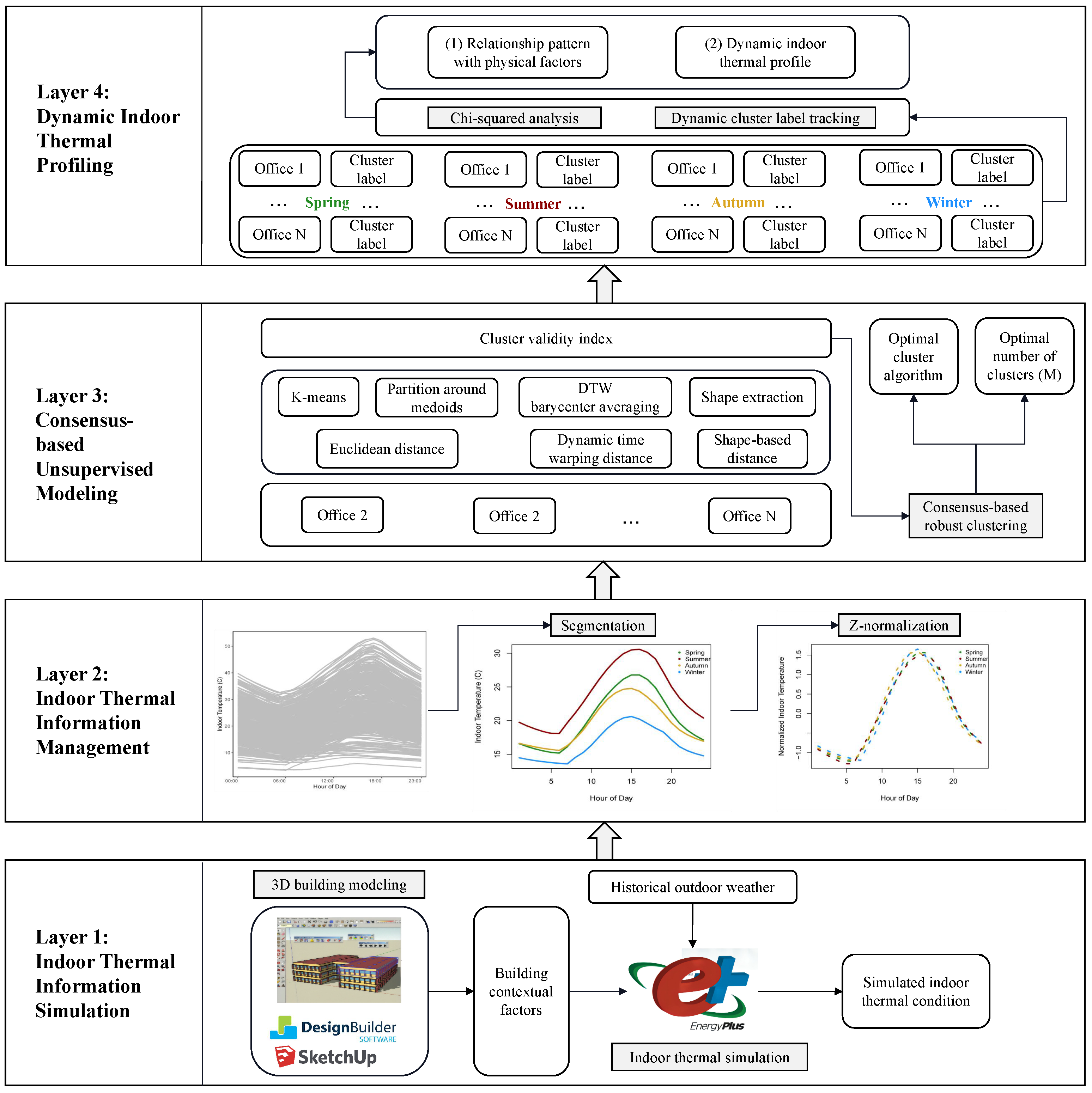
3.1. Overall Framework

In this paper, we consider a hypothetical office building in northern China where the demand for HVAC energy consumption in different seasons varies. To achieve customized building thermal control, we are interested in knowing how indoor temperature changes given different outdoor weather conditions. For an office building, it is not surprising to experience different indoor thermal conditions in different offices given the same outdoor weather conditions. Therefore, this study also aims to understand the relationship between physical factors and thermal profiles of different offices in the office building over different seasons.

A graphical overview of the system is shown in Figure 1 and explained step-by-step in Section 3.2, Section 3.3, Section 3.4 and Section 3.5. Specifically, the proposed system framework contains four layers. In layer 1 (Section 3.2), the indoor thermal information simulation process collects building physical factors, as well as indoor thermal patterns and outdoor weather conditions, which are passed to layer 2. Layer 2 (Section 3.3) then segments the thermal information for each office into seasonal time series and normalizes the thermal information to prepare it for unsupervised modeling. Subsequently, layer 3 (Section 3.4) conducts the consensus-based robust clustering to find typical thermal patterns in different time periods. Finally, layer 4 analyzes the clustering profiles including their relationship with building physical factors, and constructs the dynamic indoor thermal profiles trajectory tracking route. By analyzing cluster results, key drivers that affect indoor temperatures can be identified, which can help to develop customized thermal control strategies for each office cluster.

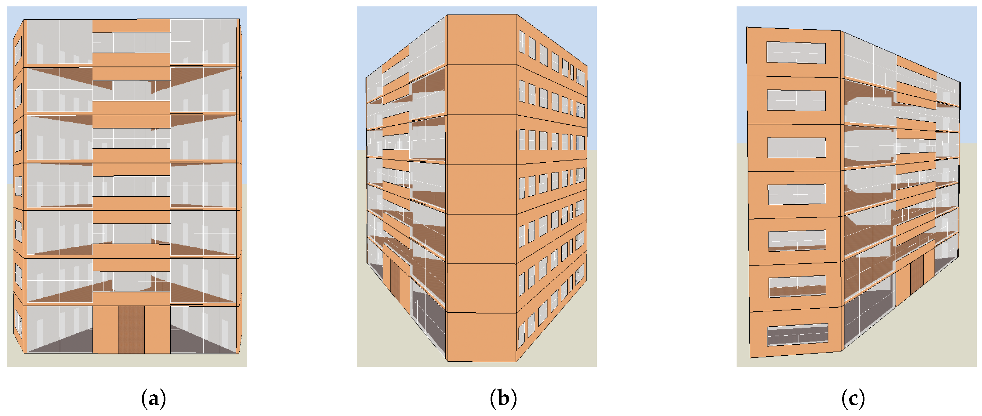
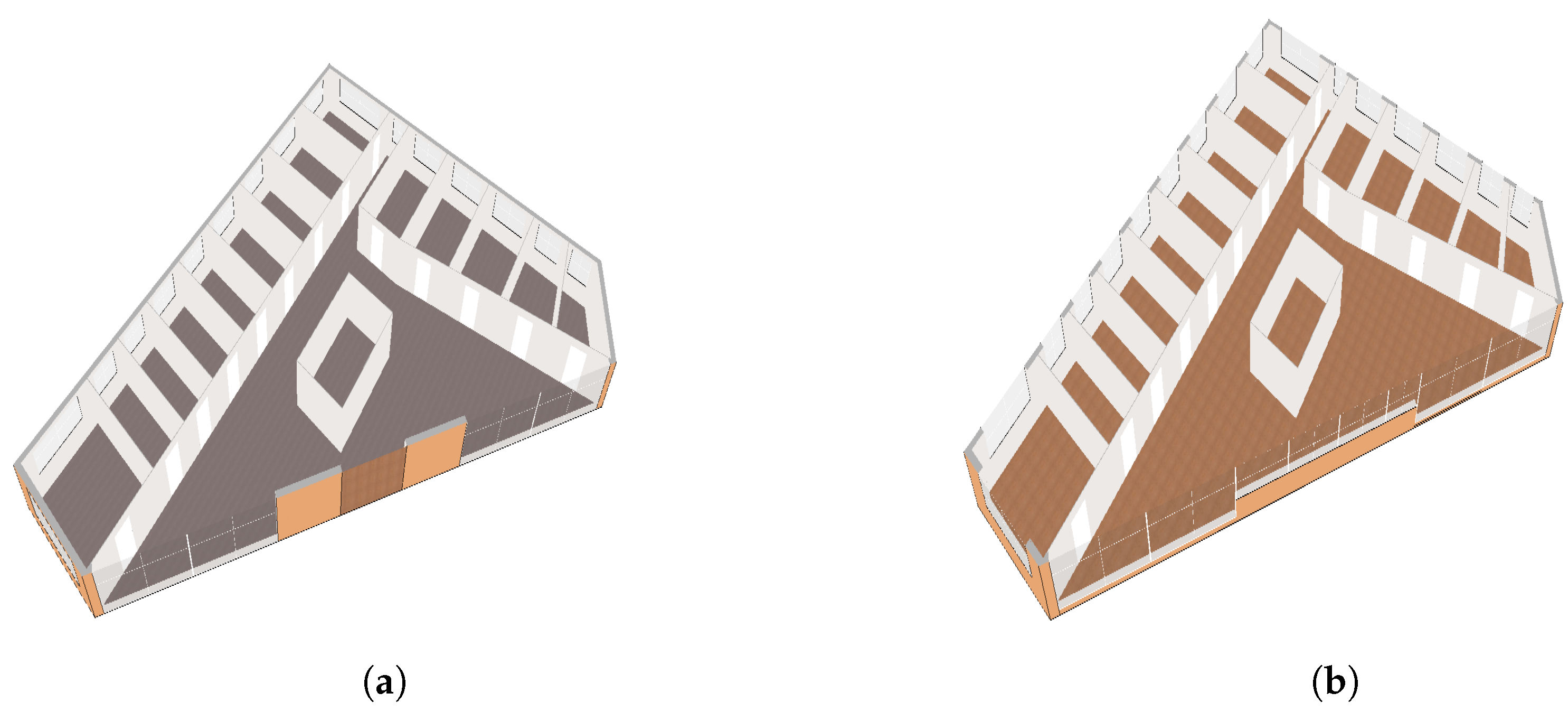
3.2. Indoor Thermal Information Simulation

The majority of existing studies on indoor thermal variation at the office level are conducted in controlled environments with thermal cameras and other expensive equipment [32]. Instead of installing various sensors to collect data from a real-world building, building simulation is a cost-effective alternative especially useful for the planning stage, e.g., in evaluating the feasibility of different technologies/concepts, and sizing of different building components. In this paper, we adopt an EnergyPlus (for simulation) and DesignBuilder (for building 3D modeling) based building simulation model to generate the hourly temperature data in each office within the building given different outdoor weather conditions.

First, a seven-floor (ground floor to sixth floor, encoded from 1 to 7 for the quantitative analysis) conceptual office building was considered as the testing case where the 3D building was modeled in DesignBuilder (see Figure 2). Each floor has 12 office rooms, and they all lie down the west and north sides of the building (see Figure 3). The office has the same room and window dimensions at the same position on different floors.

There are nine office rooms on the west side on each floor. The office rooms positioned in the middle of the west side each have one window, with the window sizes varying from 2.75 sqr.m to 5.27 sqr.m. The office room set on both ends of the west side has two windows. The south corner office on the west side has one west-facing window with a size of 5.27 sqr.m and another south-facing window with 7.20 sqr.m. The north corner office on the west side also has one west-facing window with a window size of 4.67 sqr.m and another north-facing window with 7.20 sqr.m. The office area on the west side varies from 19.15 sqr.m to 38.68 sqr.m.

Additionally, there are 3 offices on the north side on each floor. Each office has one north-facing window with a window size of about 4.1 sqr.m. Each office also has a varying room area from 28.56 sqr.m to 32.59 sqr.m.

The physical information of offices in the simulated building is summarized in

Table 1. Physical information for the simulated offices.

Physical Information	Category	Number of Offices on Each Floor	Number of Offices on Seven Floors	% of Total Number of Offices in the Building
Orientation	North	3	21	25
	West	8	56	66.7
	West/North	1	7	8.3
Floor area (m${}^2$)	19.15	2	14	16.7
	22.78	2	14	16.7
	27.04	2	14	16.7
	28.56	1	7	8.3
	31.5	1	7	8.3
	32.59	1	7	8.3
	34.22	2	14	16.7
	38.68	1	7	8.3

, where the detailed physical information for each office room is provided in Appendix A 

Table A1. Detailed physical information of office rooms.

Room Number	Floor Level	Orientation	Floor Area (m${}^2$)
Office1	Ground floor	South-West Corner	38.68
Office2	Ground floor	West	19.15
Office3	Ground floor	West	19.15
Office4	Ground floor	West	22.78
Office5	Ground floor	West	22.78
Office6	Ground floor	West	27.04
Office7	Ground floor	West	27.04
Office8	Ground floor	West	34.22
Office9	Ground floor	North-West corner	34.22
Office10	Ground floor	North	32.59
Office11	Ground floor	North	31.5
Office12	Ground floor	North	28.56
Office13	First floor	South-West Corner	38.68
Office14	First floor	West	19.15
Office15	First floor	West	19.15
Office16	First floor	West	22.78
Office17	First floor	West	22.78
Office18	First floor	West	27.04
Office19	First floor	West	27.04
Office20	First floor	West	34.22
Office21	First floor	North-West corner	34.22
Office22	First floor	North	32.59
Office23	First floor	North	31.5
Office24	First floor	North	28.56
Office25	Second floor	South-West Corner	38.68
Office26	Second floor	West	19.15
Office27	Second floor	West	19.15
Office28	Second floor	West	22.78
Office29	Second floor	West	22.78
Office30	Second floor	West	27.04
Office31	Second floor	West	27.04
Office32	Second floor	West	34.22
Office33	Second floor	North-West corner	34.22
Office34	Second floor	North	32.59
Office35	Second floor	North	31.5
Office36	Second floor	North	28.56
Office37	Third floor	South-West Corner	38.68
Office38	Third floor	West	19.15
Office39	Third floor	West	19.15
Office40	Third floor	West	22.78
Office41	Third floor	West	22.78
Office42	Third floor	West	27.04
Office43	Third floor	West	27.04
Office44	Third floor	West	34.22
Office45	Third floor	North-West corner	34.22
Office46	Third floor	North	32.59
Office47	Third floor	North	31.5
Office48	Third floor	North	28.56
Office49	Fourth floor	South-West Corner	38.68
Office50	Fourth floor	West	19.15
Office51	Fourth floor	West	19.15
Office52	Fourth floor	West	22.78
Office53	Fourth floor	West	22.78
Office54	Fourth floor	West	27.04
Office55	Fourth floor	West	27.04
Office56	Fourth floor	West	34.22
Office57	Fourth floor	North-West corner	34.22
Office58	Fourth floor	North	32.59
Office59	Fourth floor	North	31.5
Office60	Fourth floor	North	28.56
Office61	Fifth floor	South-West Corner	38.68
Office62	Fifth floor	West	19.15
Office63	Fifth floor	West	19.15
Office64	Fifth floor	West	22.78
Office65	Fifth floor	West	22.78
Office66	Fifth floor	West	27.04
Office67	Fifth floor	West	27.04
Office68	Fifth floor	West	34.22
Office69	Fifth floor	North-West corner	34.22
Office70	Fifth floor	North	32.59
Office71	Fifth floor	North	31.5
Office72	Fifth floor	North	28.56
Office73	Sixth floor	South-West Corner	38.68
Office74	Sixth floor	West	19.15
Office75	Sixth floor	West	19.15
Office76	Sixth floor	West	22.78
Office77	Sixth floor	West	22.78
Office78	Sixth floor	West	27.04
Office79	Sixth floor	West	27.04
Office80	Sixth floor	West	34.22
Office81	Sixth floor	North-West corner	34.22
Office82	Sixth floor	North	32.59
Office83	Sixth floor	North	31.5
Office84	Sixth floor	North	28.56

.

The DesignBuilder-based 3D building model was then input into EnergyPlus for thermal simulation. The default office activity schedule was applied to the associated modeled rooms while the default building regulation Part L 2013 data were applied to the construction setting of the modeled office building. HVAC systems are not included in the building model, and the indoor temperature is, therefore, only associated with building physical parameters and outside environmental parameters. After the simulation process using EnergyPlus, the whole year’s indoor thermal conditions for the modeled conceptual office building were obtained.

3.3. Indoor Thermal Information Management

To understand the typical characteristics of the obtained thermal information, we first briefly analyze the indoor temperature changes associated with different floor levels and orientations in different seasons. Figure 4 shows the average indoor temperature of offices on different floors in different seasons.

As can be observed, the ground floor has the lowest indoor temperature in spring, summer, and autumn, while it becomes the highest during the daytime in winter. Furthermore, during the transition seasons (spring and autumn), lower and middle floors (second and third floors) tend to have higher indoor temperatures. On the other hand, during summer months, the middle floors (third and fourth floors) have the highest indoor temperatures, reaching 44.01 Celsius at 17:00, while the ground floor has the coolest indoor temperature. In general, for winter months, offices on higher floors tend to be cooler (for instance, on the top floor the average room temperature at 6:00 is only 9.35 Celsius). Instead, offices on lower floors tend to be warmer in the cold season.

Based on the above seasonal segmentation, we aim to model the thermal profiles of offices in layer 3 using unsupervised learning techniques. However, it is important for these algorithms to deal with scale invariance to prioritize the shape features of the thermal patterns over amplitude features, especially for time series clustering [33,34,35]. Therefore, z-normalization was used to normalize the thermal profiles:

$$Z_i=\frac{x_i-{\mu }_i}{s_i}$$

(1)

where $Z_i$ are the normalized values calculated for all thermal profiles $x_i$ for season i. ${\mu }_i$ and $s_i$ represent the mean feature value and the standard deviation, respectively. For the seasonal thermal profiles, we use the mean feature value and the standard deviation over the season months. This will enable us to determine the dynamic trajectory of the indoor temperature profile under different weather conditions and seasons.

To assess the suitability for clustering before and after the z-normalization, we consider Hopkins’ statistical scores for the raw and z-normalized data in the four seasons, which are shown in

Table 2. Hopkins statistical scores.

	Cluster Tendency (Hopkins Statistic)
	Spring	Summer	Autumn	Winter
Raw data	0.96	0.95	0.96	0.91
Z-normalized data	0.98	0.98	0.98	0.97

. The Hopkins statistical score represents the degree of randomness in a dataset, which is calculated by comparing the sum of distances between random points in the data with the sum of distances between random points in a uniformly distributed reference set. A Hopkins score near 0.5 indicates high randomness, whereas a score near 1 (or 0) indicates high clustering (or dispersion) [36]. The results indicate that the z-normalized data produce the highest scores for all four seasons, suggesting that more meaningful clusters are present in the data set after z-normalization.

3.4. Consensus-Based Unsupervised Modeling

In layer 3, we perform clustering on the normalized seasonal indoor thermal segments. Clustering algorithms must take into account two key components, namely distance measures and prototyping functions [37]. It was demonstrated that clustering results can be unstable when only one clustering algorithm is used [38,39], and for this reason, we employ consensus-based robust clustering across multiple distance metrics and prototype combinations. Table 3 lists the clustering algorithm combinations used in this paper. Note that clustering is only one type of unsupervised learning method that could be applicable to our problem. For instance, the hierarchical Bayesian non-parametric model proposed in [40] could be considered in our future work for the problem.

The Euclidean distance [41], which approximates a one-to-one correspondence between each pair of sequences, is the most commonly used distance measure. However, for time series data (like the thermal profiles data we are considering), the distance measure needs to be invariant to specific distortions of the data to yield accurate results, which has been regarded as a limitation of the Euclidean distance [41]. Therefore, except for using the Euclidean distance, two state-of-the-art distance measures, namely the dynamic time-warping distance (DTW) [42] and the shape-based distance (SBD) [43] are also adopted in this paper to produce comprehensive similarity measures for thermal profile clustering.

To quantitatively choose the optimal number of clusters and evaluate the clustering results, three cluster validity indices (CVIs) are used in the validation process to produce robust validation results: the silhouette index, Davies–Bouldin (DB) index, and Calinski–Harabasz (CH) index. These metrics simultaneously measure the cohesion of the objects within clusters and the separation between clusters. For the silhouette index, it contrasts the average distance of objects within the same cluster to the average distance of objects in other clusters. It assumes values between −1 and 1. Cluster configurations with a higher silhouette index value are considered to be more optimal. Similarly, a higher CH index value signifies a better clustering result. In contrast, for the DB index, a lower value indicates a better clustering configuration. A more detailed description of the evaluation metrics can be found in [44,45,46].

Table 3. List of the used combination of the consensus-based clustering algorithm. DTW: dynamic time warping, SBD: shape-based distance; PAM: partition around medoids; DBA: DTW barycenter averaging.

Distance Measures	Cluster Prototypes
Euclidean Distance	K-means [47]
	PAM [48]
DTW	DBA [49]
SBD	Shape extraction [43]

Table 3. List of the used combination of the consensus-based clustering algorithm. DTW: dynamic time warping, SBD: shape-based distance; PAM: partition around medoids; DBA: DTW barycenter averaging.

Distance Measures	Cluster Prototypes
Euclidean Distance	K-means [47]
	PAM [48]
DTW	DBA [49]
SBD	Shape extraction [43]

3.5. Dynamic Indoor Thermal Profiling

After the consensus-based unsupervised modeling, a dynamic clustering structure is adopted in layer 4 to capture seasonal/dynamic changes in the indoor thermal profiles of offices. The proposed dynamic indoor thermal profiling structure is illustrated in Figure 5.

Under the dynamic profiling structure, a separate consensus-based clustering analysis is implemented for each season. The ultimate clustering results from the dynamic clustering structure consists of two components: (1) relationship pattern between the clusters and the physical factors of each office; (2) dynamic indoor thermal profile of each office.

Specifically, the clusters for different seasons are described by testing the difference in the building’s physical factors. Since the physical factors (detailed in Table 1) can all be seen as categorical variables, the chi-square test [50] is adopted to analyze the association between the clusters and the physical factors. Then, based on cluster results for each season, the dynamic indoor thermal profile for each building can be tracked, which is a cluster trajectory for each office in the building (e.g., a cluster assignment for each room under each season). More importantly, by analyzing the dynamic cluster trajectories, the corresponding physical factors possessed by the offices in each dynamic cluster trajectory can be sketched. We highlight that the proposed dynamic indoor thermal profiling layer not only allows the investigation of different thermal behaviors but also facilitates the understanding of seasonal behavioral changes.

4. Results and Analysis

In this section, we will show the results of our proposed consensus-based clustering approach, followed by the analysis of the relationship between indoor thermal patterns and building physical factors, empowered by the consensus clustering and the chi-square test. Then, the results of the dynamic indoor thermal profile recognition are discussed. For comparison purposes, we considered the benchmark case where all-seasons data are considered simultaneously, which is the most adopted approach in existing studies. In addition, to demonstrate the benefits of our proposed consensus clustering approach, performances of individual clustering algorithms are reported and compared as part of the comparative analysis.

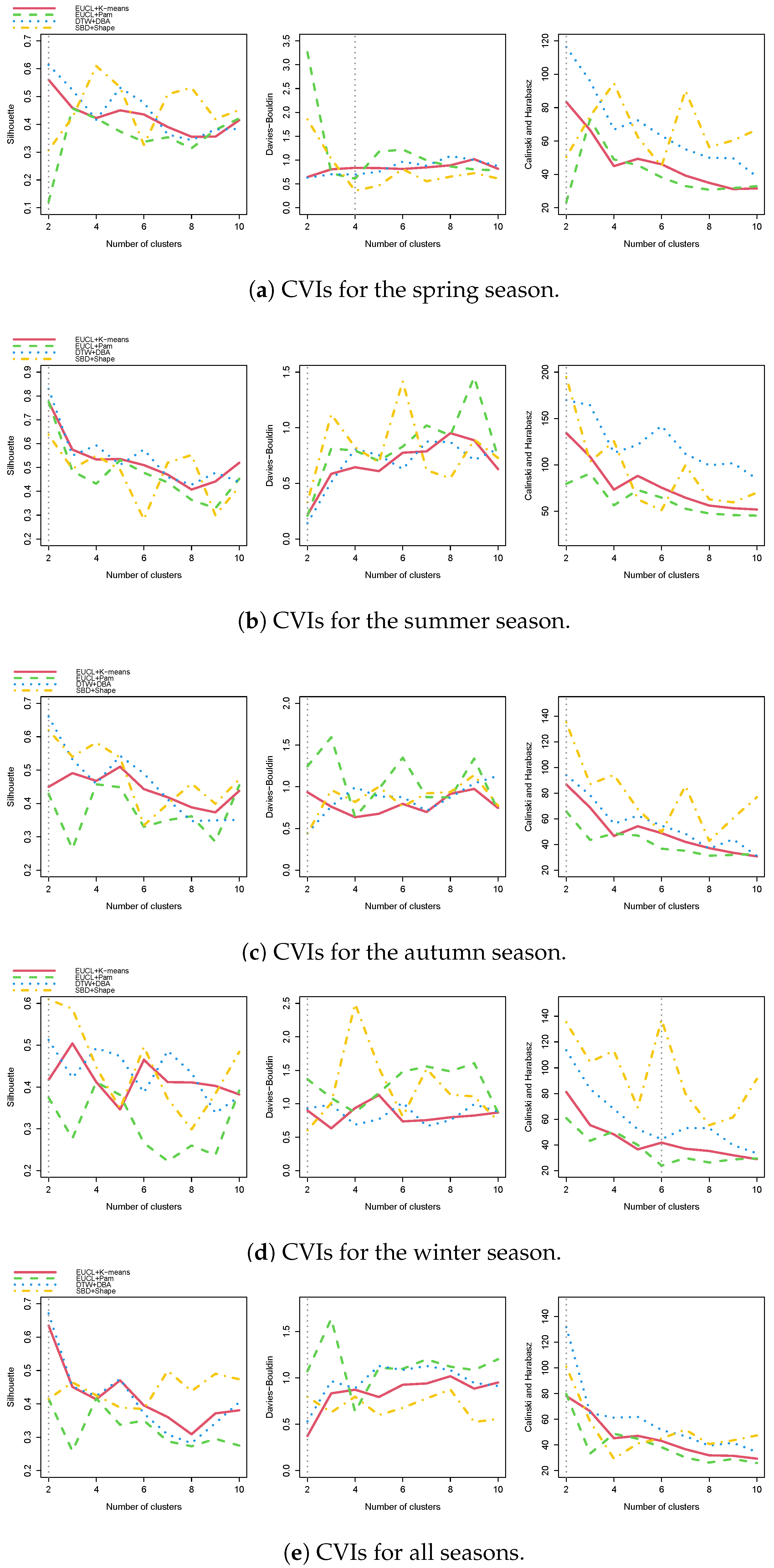
4.1. Cluster Validity Results

We adopt consensus-based clustering to cluster the 84 simulated offices based on their daily indoor temperature in different seasons. To serve as a baseline benchmark, we also consider the same clustering procedure based on all-seasons data (i.e., average thermal profile of the year rather than of each season) without differentiating different seasons. The optimal cluster number and cluster algorithm for each season and the whole year (all seasons) are chosen according to the majority vote from the three CVIs (silhouette, DB, and CH).

Specifically, we utilized tsclust in R for the consensus-based clustering process [37]. This package is specifically designed to handle the unique characteristics of time series data and offers a wide range of clustering algorithms and distance measures. We took advantage of the flexibility provided by tsclust to customize the clustering process according to our specific requirements. The parameter settings used in tsclust during our experiment are summarized in

Table 4. Parameter settings for the consensus-based clustering.

Clustering Algorithm	k	distance	centroid	window.size
Eucl. + K-means	[2:10]	Euclidean	mean	-
Eucl. + PAM	[2:10]	Euclidean	pam	-
DTW + DBA	[2:10]	dtw	dba	10
SBD + Shape extraction	[2:10]	sbd	shape	-

.

During the experiment, a random seed value (in our case, 8) was also used for reproducibility and consistency in the clustering results. We consider cluster numbers k with the range from 2 to 10. The distance measure is used to calculate the distance between time series data points, while the centroid refers to the cluster prototypes that are used to calculate the centroid for each cluster. Regarding the DTW barycenter averaging, the window.size parameter determines the size of the subsequence used for calculating the alignment path between two time series. In the experiment, a 10-h window was used to balance local patterns and the overall behavior of the time series. Figure 6 presents the visualizations of the CVIs for the cluster results in each season and the whole year (all seasons).

The CVIs offer significant insights into the quality of clustering outcomes.

Table 5. Performance comparison of clustering algorithms with the optimal cluster number in four seasons and the whole year (all-seasons data).

Spring CVIs (k = 2)
Clustering algorithm	Silhouette	DB	CH
Eucl. + K-means	0.56	0.64	83.42
Eucl. + PAM	0.12	3.26	23.26
DTW + DBA	0.61	0.63	116.25
SBD + Shape extraction	0.31	1.85	50.42
Summer CVIs (k = 2)
Clustering algorithm	Silhouette	DB	CH
Eucl. + K-means	0.78	0.22	134.24
Eucl. + PAM	0.78	0.21	79.52
DTW + DBA	0.83	0.14	169.73
SBD + Shape extraction	0.64	0.33	194.72
Autumn CVIs (k = 2)
Clustering algorithm	Silhouette	DB	CH
Eucl. + K-means	0.45	0.94	86.81
Eucl. + PAM	0.43	1.25	65.81
DTW + DBA	0.66	0.45	94.05
SBD + Shape extraction	0.62	0.44	135.20
Winter CVIs (k = 2)
Clustering algorithm	Silhouette	DB	CH
Eucl. + K-means	0.42	0.90	81.24
Eucl. + PAM	0.37	1.37	60.84
DTW + DBA	0.51	0.93	113.45
SBD + Shape extraction	0.61	0.60	135.32
All seasons CVIs (k = 2)
Clustering algorithm	Silhouette	DB	CH
Eucl. + K-means	0.63	0.37	78.07
Eucl. + PAM	0.42	1.07	79.70
DTW + DBA	0.67	0.53	131.82
SBD + Shape extraction	0.41	0.80	100.89

compares the performance of different clustering algorithms with the optimal cluster number across different seasons and the overall year, and the best scores for each algorithm are highlighted in bold.

Dynamic time-warping clustering and shape-based clustering consistently demonstrate excellent performance across all seasons. These algorithms consistently achieve higher silhouette and CH scores, indicating superior cluster separation, while also maintaining relatively low DB indices, suggesting dense and compact cluster results.

Dynamic time-warping clustering shows remarkable performance in terms of all three CVIs across spring and summer, which highlights the effectiveness of DTW clustering in capturing temporal patterns and generating meaningful clusters in each season. Similarly, shape-based clustering can capture shape-based similarities and consistently demonstrates strong performance across autumn and winter.

In contrast, traditional clustering algorithms, such as K-means and PAM, show relatively worse performance in terms of the CVIs for each season. These two algorithms generally achieve moderate silhouette scores and CH scores across all seasons. These algorithms generally achieve moderate silhouette and CH scores but tend to have higher DB indices, indicating less distinct and less dense clusters. This may be due to their limitations in capturing the inherent temporal or shape-based patterns in the time series data.

It is worth noting that the employed consensus-based approach uses multiple distance metrics (Euclidean, DTW, SBD) and prototype methods (K-means, PAM, DBA) rather than relying on a single algorithm. This approach captures different aspects of the data and reduces the bias introduced by a single algorithm. Furthermore, it enhances the robustness and stability of the clustering process compared to studies that used only a single clustering algorithm [51,52,53,54].

Moreover, evaluating cluster validity using multiple indices (silhouette, CH, DB) enables us to assess the quality and characteristics of the clusters from different perspectives, providing a more comprehensive quantitative assessment compared to many existing studies [9,30,54].

All the CVIs vote $K=2$ as the best clustering number for the indoor thermal profiles in summer and autumn. Although $K=2$ is also selected as the optimal number in spring and winter, the DB index and the CH index vote different numbers for the former and the latter, respectively. The final chosen clustering algorithms and their corresponding CVIs for each season and the whole year (benchmark) are listed in

Table 6. Lists of the optimal clustering algorithms and their corresponding CVIs for four seasons and the whole year (all-seasons data).

Season	Optimal Clustering Algorithm	Optimal Cluster Number	CVIs
			Silhouette	DB	CH
Spring	DTW + DBA	2	0.61	0.63	116.25
Summer	DTW + DBA	2	0.83	0.14	169.73
Autumn	SBD + Shape extraction	2	0.62	0.44	135.20
Winter	SBD + Shape extraction	2	0.61	0.60	135.32
All seasons	DTW + DBA	2	0.67	0.53	131.82

.

Finally, dynamic time-warping clustering is selected to generate two clusters for the spring and summer seasons, respectively. The same choice was made for the clustering of all-year data (all seasons). The K-shape utilizing the SBD distance and the shape extraction prototype is applied to produce two clusters for the autumn and winter seasons. Figure 7 illustrates the cluster centroids for each of four seasons and the whole year (all seasons).

4.2. Relationship Pattern between Seasonal Indoor Thermal Clusters and Physical Factors

Using the consensus clustering results, the chi-square test is performed to test differences in different clusters according to building physical factors (floor level, floor area, orientation) during different seasons. To serve as a benchmark, the chi-square test has also been conducted for the consensus clustering results based on the all-year data (all seasons). The detailed test results for three building physical variables are provided in Appendix B 

Table A2. Chi-square test results for spring clusters.

Variable	Category	Clusters		Test Results
		Cluster 1	Cluster 2	${\mathit{x}}^{\mathbf{2}}$	$\mathit{p}$
Floor level	Ground floor	12	0	55.519	0.000 ***
	First floor	5	7
	Second floor	0	12
	Third floor	0	12
	Fourth floor	0	12
	Fifth floor	0	12
	Sixth floor	3	9
Floor area m${}^2$	19.15	2	12	6.431	0.490
	22.78	2	12
	27.04	2	12
	28.56	3	4
	31.5	3	4
	32.59	2	5
	34.22	5	9
	38.68	1	6
Orientation	North	8	13	5.611	0.060
	West	9	47
	West/North	3	4

*** p < 0.01.

,

Table A3. Chi-square test results for summer clusters.

Variable	Category	Clusters		Test Results
		Cluster 1	Cluster 2	${\mathit{x}}^{\mathbf{2}}$	$\mathit{p}$
Floor level	Ground floor	12	0	84	0.000 ***
	First floor	0	12
	Second floor	0	12
	Third floor	0	12
	Fourth floor	0	12
	Fifth floor	0	12
	Sixth floor	0	12
Floor area m${}^2$	19.15	2	12	0.000	1
	22.78	2	12
	27.04	2	12
	28.56	1	4
	31.5	1	4
	32.59	1	5
	34.22	2	9
	38.68	1	6
Orientation	North	3	18	0.000	1
	West	8	48
	West/North	1	6

*** p< 0.01.

,

Table A4. Chi-square test results for autumn clusters.

Variable	Category	Clusters		Test Results
		Cluster 1	Cluster 2	${\mathit{x}}^{\mathbf{2}}$	$\mathit{p}$
Floor level	Ground floor	0	12	15.515	0.017 **
	First floor	9	3
	Second floor	6	6
	Third floor	4	8
	Fourth floor	4	8
	Fifth floor	5	7
	Sixth floor	6	6
Floor area m${}^2$	19.15	4	10	38.936	0.000 ***
	22.78	0	14
	27.04	4	10
	28.56	1	6
	31.5	1	6
	32.59	6	1
	34.22	12	2
	38.68	6	1
Orientation	North	8	13	6.522	0.038 **
	West	20	36
	West/North	6	1

*** p < 0.01, ** p < 0.05.

,

Table A5. Chi-square test results for winter clusters.

Variable	Category	Clusters		Test Results
		Cluster 1	Cluster 2	${\mathit{x}}^{\mathbf{2}}$	$\mathit{p}$
Floor level	Ground floor	0	12	52.871	0.000 ***
	First floor	11	1
	Second floor	12	0
	Third floor	12	0
	Fourth floor	8	4
	Fifth floor	6	6
	Sixth floor	1	11
Floor area m${}^2$	19.15	9	5	6.028	0.536
	22.78	6	8
	27.04	9	5
	28.56	3	4
	31.5	5	2
	32.59	5	2
	34.22	7	7
	38.68	6	1
Orientation	North	13	8	3.039	0.219
	West	35	21
	West/North	2	5

*** p < 0.01.

and

Table A6. Chi-square test results for clusters of all seasons.

Variable	Category	Clusters		Test Results
		Cluster 1	Cluster 2	${\mathit{x}}^{\mathbf{2}}$	$\mathit{p}$
Floor level	Ground floor	12	0	66.706	0.000 ***
	First floor	4	8
	Second floor	0	12
	Third floor	0	12
	Fourth floor	0	12
	Fifth floor	0	12
	Sixth floor	0	12
Floor area m${}^2$	19.15	4	10	2.007	0.959
	22.78	3	11
	27.04	2	12
	28.56	1	6
	31.5	1	6
	32.59	1	6
	34.22	2	12
	38.68	2	5
Orientation	North	3	18	0.618	0.734
	West	12	44
	West/North	1	6

*** p < 0.01.

.

Several high-level distinct patterns can be observed, which is not possible without differentiating among different seasons. In particular, the dynamic impact of physical factors on the indoor temperature in different seasons can be identified through our proposed approach. That is, a certain physical factor (e.g., floor level, floor area, or orientation) could be the main factor for one season but less important in other seasons. To be more specific, based on the chi-square test results, a statistically significant association between clusters and floor levels in the spring season is observed. For instance, cluster 1 mainly consists of offices on the ground and first floors (see Table A2). Most of the small offices are located in cluster 2, with the majority of offices located to the west. Similarly, the association between clusters and floor levels is found to be significant for the summer season with cluster 1 consisting of all the offices on the ground floor. In fact, the floor level is the dominant factor for the indoor temperature in the summer season (see Table A3). Interestingly, all three physical factors are significantly associated with the autumn season. Among the three physical factors, floor area seems to be the dominant factor with small offices primarily located in cluster 2. In addition, the physical factor of office orientation is only found to be significant for the autumn season with almost all offices in cluster 2 facing either North or West (see Table A4). For the winter season, the association between clusters and the floor levels is found to be significant with cluster 2 including all the offices on the ground floor and almost all the offices on the sixth floor (top floor) (see Table A5). In contrast, the chi-square test results based on the clustering of all-seasons data indicate only floor level is significantly associated. In particular, cluster 1 consists of offices on the ground floor and first floor only (see Table A6).

To better understand the changing patterns in clusters over different seasons and their dynamic association with different physical factors, the corresponding average physical factors are utilized to reflect common building characteristics in each cluster, as shown in

Table 7. Clusters profile summary for different seasons and the whole year (all seasons).

Cluster	Floor Level	Floor Area	Mean Temp.	Max/Min Temp.	Cluster Label
Spring
1	2.15	29.65	21.14	26.66/16.11	Low floor level; medium office size; lower indoor temperature.
2	4.58	27.67	25.13	32.55/18.44	Medium floor level; medium office size; higher indoor temperature.
Summer
1	1.00	28.14	23.11	28.02/18.61	Low floor level; medium office size; lower indoor temperature.
2	4.50	28.14	34.41	42.61/26.89	Medium floor level; medium office size; higher indoor temperature.
Autumn
1	4.24	31.86	22.42	28.57/16.74	Medium floor level; large office size; higher indoor temperature.
2	3.84	25.62	21.98	26.55/17.67	Low–Medium floor level; small office size; lower indoor temperature.
Winter
1	3.78	28.60	15.22	19.52/10.82	Low–Medium floor level; medium office size; higher indoor temperature.
2	4.32	27.47	14.97	18.50/11.44	Medium floor level; medium office size; lower indoor temperature.
All seasons
1	1.25	27.34	20.69	25.34/16.56	low floor level; medium office size; lower indoor temperature.
2	4.65	28.33	24.30	30.56/18.50	Medium floor level; medium office size; higher indoor temperature.

. Moreover, the mean, minimum, and maximum indoor temperatures of offices within each cluster are also summarized for each of the four seasons to facilitate tracking of the dynamic cluster trajectory for each office. We can conclude from the results of clustering and the physical information of the buildings that there is a distinct characteristic associated with each cluster, as indicated in the cluster labels. In generating the cluster labels, floors are divided into three categories: low (ground to second floors, i.e., 1–3), medium (third and fourth floors, i.e., 4–5), and high (fifth and sixth floors, i.e., 6–7).

We can observe that during the spring season, cluster 1 has low floor levels, medium-sized offices, and lower indoor temperatures. In contrast, cluster 2 has medium floor levels, medium office sizes, and a higher daily indoor temperature. During the summer, cluster 1 is associated with low floor levels and a cooler indoor temperature, while cluster 2 has medium floor levels and higher indoor temperature with a maximum temperature of 42.61 Celsius. In autumn, cluster 1 has a medium floor level, a large office size, and a warmer indoor temperature, while cluster 2 has a low–medium floor level, small offices, and a cooler indoor temperature. In winter months, cluster 1 has low–medium floor level, medium floor area, and slightly higher indoor temperature, while cluster 2 has a medium floor level, a medium floor area, and a lower indoor temperature. It is also observed that the differences in average indoor temperatures in the two clusters for the autumn and winter seasons are less distinct than other seasons. To summarize, based on our approach, the clustering results over four seasons generate six distinct cluster profiles (six distinct cluster labels). In contrast, the clustering based on all-seasons data only results in two clusters (i.e., two distinct cluster labels), where cluster 1 has a low floor level, medium office area, and lower indoor temperature, and cluster 2 has a medium floor level, medium office size, and higher indoor temperature.

Based on the above analysis, we can observe distinct thermal performances and behaviors of offices in different seasons and underlying physical factors. In other words, the same offices may behave differently in different seasons, affected by different physical factors differently over time.

4.3. Dynamic Indoor Thermal Profile Recognition

In order to track the dynamic cluster trajectory for the offices (i.e., track different behavior patterns in different seasons), a category summary is performed after characterizing each cluster for each season.

Table 8. Category summary for the dynamic cluster trajectories over the year. DT: dynamic trajectory.

Spring Cluster	Summer Cluster	Autumn Cluster	Winter Cluster	Floor Level	Floor Area	Mean Temp.	DT No.
1	1	2	2	1 (low)	28.14 (med.)	19.58	1
	2	1	1	2 (low)	31.72 (large)	22.53	2
		1	2	4.50 (med.)	34.22 (large)	22.79	3
		2	2	7 (high)	30.03 (med.)	23.42	4
2	2	1	1	4 (med.)	32.11 (large)	24.56	5
		1	2	6.50 (high)	30.24 (med.)	24.14	6
		2	1	3.88 (low–med.)	24.87 (small)	24.68	7
		2	2	6.08 (high)	23.85 (small)	24.69	8

summarizes all cluster trajectories that exist based on clustering results over four different seasons in the previous subsection, together with the average thermal profile of each trajectory. In total, eight dynamic trajectories (DTs) were identified for the 84 simulated offices, and the characteristics of each DT can be summarized by combining the cluster labels for each season defined in Table 7. For instance, for offices following DT 1, they appear in cluster 1 (lower temperature according to Table 7) in the spring season, remain in cluster 1 (lower temperature) for the summer season but change to cluster 2 (lower temperatures) in the autumn and winter seasons. That is, the offices following DT 1 have relatively lower indoor temperature throughout the year, characterized by low floor levels and medium floor areas. The detailed offices that follow each dynamic trajectory (DT) are listed in Appendix B 

Table A7. List of offices in the eight DTs.

DT 1	DT 2	DT 3	DT 4	DT 5	DT 6	DT 7	DT 8
Office1	Office20	Office21	Office83	Office13	Office57	Office15	Office52
Office2	Office22	Office81	Office84	Office14	Office69	Office16	Office53
Office3	Office23			Office18	Office74	Office17	Office60
Office4	Office24			Office19	Office79	Office27	Office63
Office5				Office25	Office80	Office28	Office64
Office6				Office26	Office82	Office29	Office65
Office7				Office31		Office30	Office66
Office8				Office32		Office35	Office72
Office9				Office33		Office36	Office75
Office10				Office34		Office38	Office76
Office11				Office37		Office39	Office77
Office12				Office44		Office40	Office78
				Office45		Office41
				Office46		Office42
				Office49		Office43
				Office56		Office47
				Office58		Office48
				Office61		Office50
				Office62		Office51
				Office68		Office54
				Office70		Office55
				Office73		Office59
						Office67
						Office71

.

In general, there are low floor levels in both DT 1 and DT 2, with DT 1 containing medium offices and DT 2 containing large offices. Most offices that follow DTs 3, 5, and 7 are located on medium floor levels, and offices in DTs 3 and 5 have large floor areas. On the other hand, DT 7, which has the largest number of offices, is characterized by low to medium floor levels and small office sizes. Furthermore, most offices following DTs 4, 6, and 8 are located on the upper floors. In addition, those who follow DTs 4 and 6 have a medium-sized office, while those who follow DT 8 have a small-sized office.

Based on the characteristics described in each DT, the dynamic thermal behavior can be summarized, and useful managerial insights (MIs) can be gained to assist the building manager/operator in developing customized thermal control strategies:

• MIs for DT 1. Offices following DT 1 experience lower indoor temperatures throughout the year than offices following other DTs. As these offices experience a cooler winter, thermal control decisions should be made with additional consideration for DT 1 during this period.
• MIs for DT 2. The indoor temperature of offices following DT 2 is lower in the spring and higher from the summer to the winter. It is, therefore, necessary for the thermal control system to cool the offices that follow DT 2 during the summer months to ensure optimal comfort for the occupants.
• MIs for DT 3. In DT 3, offices experience lower indoor temperatures during winter and spring, and higher indoor temperatures during summer and autumn. Consequently, offices following DT 3 require special attention to the thermal control system during the summer and winter months as occupants suffer from high indoor temperatures in the summer and low indoor temperatures in the winter. In addition, it expects extended operations of thermal control systems in transition seasons due to higher temperatures in the autumn and lower temperatures in the spring.
• MIs for DT 4. In DT 4, offices experience higher indoor temperatures in the summer and lower indoor temperatures in the winter and two transition seasons (spring and autumn). As in DT 3, the thermal control system should ensure that the offices in DT 4 are maintained at a comfortable temperature throughout the summer and winter.
• MIs for DT 5. Offices in DT 5 are generally warmer throughout the year. Similar to DT 2, DT 5 requires the thermal control system to maintain a comfortable temperature during the summer months.
• MIs for DT 6. As in DTs 3 and 4, offices in DT 6 also experience higher indoor temperatures during the summer and two transition seasons and lower indoor temperatures during the winter. Therefore, the thermal control system in DT 6 should optimize thermal comfort for the offices during the summer and winter seasons.
• MIs for DT 7. In offices following DT 7, the indoor temperature is lower during autumn and higher during other seasons, especially during the summer. Thermal control systems should, therefore, ensure that the indoor temperatures in DT 7 do not become excessively hot during the summer months.
• MIs for DT 8. As with DTs 3, 4, and 6, offices in DT 8 also experience higher summer temperatures and lower winter temperatures. Therefore, the thermal control system in DT 8 should enable offices to remain comfortably cool during the summer and warm during the winter. However, DT 8 presents a unique trajectory with higher temperatures in the spring and lower temperatures in the autumn.

It can be observed that offices following DTs 3, 4, 6, and 8 experience higher summer temperatures and lower winter temperatures. Therefore, thermal control strategies can be developed in order to optimize the thermal comfort of these offices in both seasons. Moreover, offices following DTs 2, 5, and 7 require thermal comfort optimization strategies during the summer, while offices following DT 1 require thermal comfort optimization strategies during the winter. Although some DTs (e.g., DTs 3, 4, 6, 8) seem to present similar thermal behaviors in summer and winter seasons, they have distinct patterns during two transition seasons (i.e., spring and autumn). Overall, each DT presents a unique trajectory with its own characteristics, which could provide useful insights and opportunities for customized building operation and management.

4.4. Discussion

In light of the above analysis, we can conclude that there are different physical factors contributing to thermal differences among offices in different seasons. Furthermore, the dynamic cluster trajectory of the offices provides valuable guidance for designing customized building climate control strategies. Although we considered a case study focusing on different rooms/offices within a single building, it is worth mentioning that the proposed method can be readily extended or easily modified to other different built environment settings at different spatial-temporal scales such as examining behaviors of different types of buildings or a group of buildings. When performing the analysis for a group of different types of buildings simultaneously (e.g., a district or city level), we could consider extending the current simulation model by including more building physical factors (e.g., building material, insulation, etc.) to account for the difference between buildings.

Moreover, the above promising results can also be applied to other relevant applications, such as for the building energy management/energy pricing and accounting for economic benefits of building retrofits. As for the former, based on the customized data-driven building’s indoor thermal profiles, customized HVAC control and the energy management approach can be developed for each office/each group of offices, considering the differences in thermal performance. It is also possible to consider customized energy pricing and demand response management strategies in similar application scenarios (e.g., for a group of buildings) to manage the energy costs. For the latter, it can be achieved by using the developed clustering-based indoor thermal performance profiling system, allowing different building retrofit plans to be evaluated through simulations on a group of rooms/buildings rather than on individual rooms/buildings, which can then be incorporated into an economic benefit analysis to obtain the optimal building retrofit plan. According to the above, the proposed smart building indoor thermal profiling system can lead to promising computational benefits, as the consensus-based clustering method can significantly reduce the number of simulations required, which is particularly useful for large and complex buildings and big data scenarios.

5. Conclusions

This paper proposes an indoor thermal profiling system for smart buildings that is useful for customized thermal control in buildings. Firstly, a building simulation model based on EnergyPlus is developed to simulate the thermal conditions of individual offices under various outdoor weather conditions. Secondly, the simulated thermal conditions are segmented and normalized based on the different seasons throughout the year. To capture different building thermal behaviors in different seasons, the consensus-based robust clustering approach is applied to cluster individual offices into different groups. By analyzing clustering results with accompanying building physical information, we are able to identify underlying factors that can explain the observed thermal performance behaviors, which is an important step toward developing a fully automated customized building climate control system. Moreover, the dynamic cluster trajectories of the simulated 84 offices are summarized to provide valuable guidance for designing different building climate control strategies for different times of the year. The promising results shown in our experimental analysis will inspire future directions of our work; we aim to further develop and extend our proposed methodological framework to other areas, such as customized building energy management, energy pricing, and economic benefit analysis of building retrofits and design. For instance, different thermal behaviors of offices (assuming multiple companies/organizations share the same building in this example) can be taken into account when offering different energy tariffs to different companies/organizations by the load serving entity (LSE), to incentivize the best energy use behaviors, such as reducing emissions and energy bills. Another potential area of our proposed framework is to study the potential impact of different building retrofit designs on indoor thermal behavior in order to evaluate its impact on overall energy efficiency.

References

1. Global Alliance for Buildings and Construction, International Energy Agency and the United Nations Environment Programme. 2019 Global Status Report for Buildings and Construction: Towards a Zero-Emission, Efficient and Resilient Buildings and Construction Sector; United Nations Environment Programme Nairobi: Nairobi, Kenya, 2019; Available online: https://www.iea.org/reports/global-status-report-for-buildings-and-construction-2019 (accessed on 1 March 2023).
2. Levesque, A.; Pietzcker, R.C.; Luderer, G. Halving energy demand from buildings: The impact of low consumption practices. Technol. Forecast. Soc. Chang. 2019, 146, 253–266. [Google Scholar] [CrossRef]
3. Li, H.X.; Li, Y.; Jiang, B.; Zhang, L.; Wu, X.; Lin, J. Energy performance optimisation of building envelope retrofit through integrated orthogonal arrays with data envelopment analysis. Renew. Energy 2020, 149, 1414–1423. [Google Scholar] [CrossRef]
4. Lex, S.W.; Calì, D.; Rasmussen, M.K.; Bacher, P.; Bachalarz, M.; Madsen, H. A cross-disciplinary path to healthy and energy efficient buildings. Technol. Forecast. Soc. Chang. 2019, 142, 273–284. [Google Scholar] [CrossRef]
5. Chen, C.; Wang, J.; Heo, Y.; Kishore, S. MPC-based appliance scheduling for residential building energy management controller. IEEE Trans. Smart Grid 2013, 4, 1401–1410. [Google Scholar] [CrossRef]
6. Wang, J.; Li, S.; Chen, H.; Yuan, Y.; Huang, Y. Data-driven model predictive control for building climate control: Three case studies on different buildings. Build. Environ. 2019, 160, 106204. [Google Scholar] [CrossRef]
7. Le, D.N.; Le Tuan, L.; Tuan, M.N.D. Smart-building management system: An Internet-of-Things (IoT) application business model in Vietnam. Technol. Forecast. Soc. Chang. 2019, 141, 22–35. [Google Scholar] [CrossRef]
8. Zheng, G.; Wei, C.; Yue, X.; Li, K. Application of hierarchical cluster analysis in age segmentation for thermal comfort differentiation of elderly people in summer. Build. Environ. 2023, 230, 109981. [Google Scholar] [CrossRef]
9. Bueno, A.M.; da Luz, I.M.; Niza, I.L.; Broday, E.E. Hierarchical and K-means clustering to assess thermal dissatisfaction and productivity in university classrooms. Build. Environ. 2023, 233, 110097. [Google Scholar] [CrossRef]
10. Kim, J.; Zhou, Y.; Schiavon, S.; Raftery, P.; Brager, G. Personal comfort models: Predicting individuals’ thermal preference using occupant heating and cooling behavior and machine learning. Build. Environ. 2018, 129, 96–106. [Google Scholar] [CrossRef]
11. Jazizadeh, F.; Jung, W. Personalized thermal comfort inference using RGB video images for distributed HVAC control. Appl. Energy 2018, 220, 829–841. [Google Scholar] [CrossRef]
12. Liu, S. Personal thermal comfort models based on physiological parameters measured by wearable sensors. In Proceedings of the 10th Windsor Conference: Rethinking Comfort, NCEUB, Windsor, UK, 12–15 April 2018; pp. 1–11. [Google Scholar]
13. Li, D.; Menassa, C.C.; Kamat, V.R. Personalized human comfort in indoor building environments under diverse conditioning modes. Build. Environ. 2017, 126, 304–317. [Google Scholar] [CrossRef]
14. Abdelrahman, M.M.; Chong, A.; Miller, C. Personal thermal comfort models using digital twins: Preference prediction with BIM-extracted spatial–temporal proximity data from Build2Vec. Build. Environ. 2022, 207, 108532. [Google Scholar] [CrossRef]
15. Jia, M.; Srinivasan, R. Building Performance Evaluation Using Coupled Simulation of EnergyPlus™ and an Occupant Behavior Model. Sustainability 2020, 12, 4086. [Google Scholar] [CrossRef]
16. Hensen, J.L.; Lamberts, R. Building Performance Simulation for Design and Operation; Routledge: London, UK, 2012. [Google Scholar]
17. Yao, L.; Chini, A.; Zeng, R. Integrating cost-benefits analysis and life cycle assessment of green roofs: A case study in Florida. Hum. Ecol. Risk Assess. Int. J. 2020, 26, 443–458. [Google Scholar] [CrossRef]
18. Anastasiadi, C.; Dounis, A.I. Co-simulation of fuzzy control in buildings and the HVAC system using BCVTB. Adv. Build. Energy Res. 2018, 12, 195–216. [Google Scholar] [CrossRef]
19. Alonso, M.J.; Dols, W.S.; Mathisen, H. Using Co-simulation between EnergyPlus and CONTAM to evaluate recirculation-based, demand-controlled ventilation strategies in an office building. Build. Environ. 2022, 211, 108737. [Google Scholar] [CrossRef]
20. Wei, S.; Jones, R.; De Wilde, P. Driving factors for occupant-controlled space heating in residential buildings. Energy Build. 2014, 70, 36–44. [Google Scholar] [CrossRef]
21. Bruce-Konuah, A.; Jones, R.V.; Fuertes, A. Physical environmental and contextual drivers of occupants’ manual space heating override behaviour in UK residential buildings. Energy Build. 2019, 183, 129–138. [Google Scholar] [CrossRef]
22. Sen, A.; Qiu, Y. Aggregate Household Behavior in Heating and Cooling Control Strategy and Energy-Efficient Appliance Adoption. IEEE Trans. Eng. Manag. 2022, 69, 682–696. [Google Scholar] [CrossRef]
23. Pivac, N.; Nižetić, S.; Zanki, V. Occupant behavior and thermal comfort field analysis in typical educational research institution: A case study. Therm. Sci. 2018, 22, 785–795. [Google Scholar] [CrossRef]
24. Schweiker, M.; Ampatzi, E.; Andargie, M.S.; Andersen, R.K.; Azar, E.; Barthelmes, V.M.; Berger, C.; Bourikas, L.; Carlucci, S.; Chinazzo, G.; et al. Review of multi-domain approaches to indoor environmental perception and behaviour. Build. Environ. 2020, 176, 106804. [Google Scholar] [CrossRef]
25. Lu, S.; Gu, W.; Ding, S.; Yao, S.; Lu, H.; Yuan, X. Data-Driven aggregate thermal dynamic model for buildings: A regression approach. IEEE Trans. Smart Grid 2021, 13, 227–242. [Google Scholar] [CrossRef]
26. Buttitta, G.; Turner, W.; Finn, D. Clustering of household occupancy profiles for archetype building models. Energy Procedia 2017, 111, 161–170. [Google Scholar] [CrossRef]
27. Green, R.; Staffell, I.; Vasilakos, N. Divide and Conquer? k-Means Clustering of Demand Data Allows Rapid and Accurate Simulations of the British Electricity System. IEEE Trans. Eng. Manag. 2014, 61, 251–260. [Google Scholar] [CrossRef]
28. Laskari, M.; Karatasou, S.; Santamouris, M.; Assimakopoulos, M.N. Using pattern recognition to characterise heating behaviour in residential buildings. Adv. Build. Energy Res. 2022, 16, 322–346. [Google Scholar] [CrossRef]
29. Nikolaou, T.G.; Kolokotsa, D.S.; Stavrakakis, G.S.; Skias, I.D. On the application of clustering techniques for office buildings’ energy and thermal comfort classification. IEEE Trans. Smart Grid 2012, 3, 2196–2210. [Google Scholar] [CrossRef]
30. Wickramasinghe, A.; Muthukumarana, S.; Loewen, D.; Schaubroeck, M. Temperature clusters in commercial buildings using k-means and time series clustering. Energy Inform. 2022, 5, 1. [Google Scholar] [CrossRef]
31. Asumadu-Sakyi, A.; Miller, W.; Barnett, A.; Thai, P.; Jayaratne, E.; Thompson, M.; Roghani, R.; Morawska, L. Seasonal temperature patterns and durations of acceptable temperature range in houses in Brisbane, Australia. Sci. Total Environ. 2019, 683, 470–479. [Google Scholar] [CrossRef]
32. Barreira, E.; Almeida, R.M.; Moreira, M. An infrared thermography passive approach to assess the effect of leakage points in buildings. Energy Build. 2017, 140, 224–235. [Google Scholar] [CrossRef]
33. Javed, A.; Lee, B.S.; Rizzo, D.M. A benchmark study on time series clustering. Mach. Learn. Appl. 2020, 1, 100001. [Google Scholar] [CrossRef]
34. Deng, X.; Tan, Z.; Tan, M.; Chen, W. A clustering-based climatic zoning method for office buildings in China. J. Build. Eng. 2021, 42, 102778. [Google Scholar] [CrossRef]
35. Xu, J.; Kang, X.; Chen, Z.; Yan, D.; Guo, S.; Jin, Y.; Hao, T.; Jia, R. Clustering-based probability distribution model for monthly residential building electricity consumption analysis. Build. Simul. 2021, 14, 149–164. [Google Scholar] [CrossRef]
36. Hopkins, B.; Skellam, J.G. A new method for determining the type of distribution of plant individuals. Ann. Bot. 1954, 18, 213–227. [Google Scholar] [CrossRef]
37. Montero, P.; Vilar, J.A. TSclust: An R Package for Time Series Clustering. J. Stat. Softw. 2014, 62, 1–43. [Google Scholar] [CrossRef]
38. Hsu, D. Comparison of integrated clustering methods for accurate and stable prediction of building energy consumption data. Appl. Energy 2015, 160, 153–163. [Google Scholar] [CrossRef]
39. Satre-Meloy, A.; Diakonova, M.; Grünewald, P. Cluster analysis and prediction of residential peak demand profiles using occupant activity data. Appl. Energy 2020, 260, 114246. [Google Scholar] [CrossRef]
40. Fan, W.; Yang, L.; Bouguila, N. Unsupervised grouped axial data modeling via hierarchical bayesian nonparametric models With watson distributions. IEEE Trans. Pattern Anal. Mach. Intell. 2022, 44, 9654–9668. [Google Scholar] [CrossRef]
41. Keogh, E.; Ratanamahatana, A. Everything you know about dynamic time warping is wrong. In Proceedings of the 3rd International Workshop on Mining Temporal and Sequential Data, Seattle, DC, USA, 22 August 2004; pp. 1–11. [Google Scholar]
42. Berndt, D.J.; Clifford, J. Using Dynamic Time Warping to Find Patterns in Time Series. In Proceedings of the 3rd International Conference on Knowledge Discovery and Data Mining, Seattle, WA, USA, 31 July–1 August 1994; AAAI Press: Menlo Park, CA, USA, 1994; pp. 359–370. [Google Scholar]
43. Paparrizos, J.; Gravano, L. k-shape: Efficient and accurate clustering of time series. In Proceedings of the 2015 ACM SIGMOD International Conference on Management of Data, Victoria, Australia, 31 May–4 June 2015; pp. 1855–1870. [Google Scholar]
44. de Zepeda, M.V.N.; Meng, F.; Su, J.; Zeng, X.J.; Wang, Q. Dynamic clustering analysis for driving styles identification. Eng. Appl. Artif. Intell. 2021, 97, 104096. [Google Scholar] [CrossRef]
45. Sardá-Espinosa, A. Time-Series Clustering in R Using the dtwclust Package. R J. 2019, 11, 22. [Google Scholar] [CrossRef]
46. Meng, F.; Ma, Q.; Liu, Z.; Zeng, X.J. Multiple dynamic pricing for demand response with adaptive clustering-based customer segmentation in smart grids. Appl. Energy 2023, 333, 120626. [Google Scholar] [CrossRef]
47. Lloyd, S. Least squares quantization in PCM. IEEE Trans. Inf. Theory 1982, 28, 129–137. [Google Scholar] [CrossRef]
48. Rdusseeun, L.; Kaufman, P. Clustering by means of medoids. In Proceedings of the Statistical Data Analysis Based on the L1 Norm Conference, Neuchatel, Switzerland, 4–9 August 1987; Volume 31. [Google Scholar]
49. Petitjean, F.; Ketterlin, A.; Gançarski, P. A global averaging method for dynamic time warping, with applications to clustering. Pattern Recognit. 2011, 44, 678–693. [Google Scholar] [CrossRef]
50. Pearson, K.X. On the criterion that a given system of deviations from the probable in the case of a correlated system of variables is such that it can be reasonably supposed to have arisen from random sampling. Lond. Edinb. Dublin Philos. Mag. J. Sci. 1900, 50, 157–175. [Google Scholar] [CrossRef]
51. Zhang, G.; Li, Y.; Deng, X. K-means clustering-based electrical equipment identification for smart building application. Information 2020, 11, 27. [Google Scholar] [CrossRef]
52. Gianniou, P.; Liu, X.; Heller, A.; Nielsen, P.S.; Rode, C. Clustering-based analysis for residential district heating data. Energy Convers. Manag. 2018, 165, 840–850. [Google Scholar] [CrossRef]
53. Et-taleby, A.; Boussetta, M.; Benslimane, M. Faults detection for photovoltaic field based on k-means, elbow, and average silhouette techniques through the segmentation of a thermal image. Int. J. Photoenergy 2020, 2020, 6617597. [Google Scholar] [CrossRef]
54. Nazir, A.; Wajahat, A.; Akhtar, F.; Ullah, F.; Qureshi, S.; Malik, S.A.; Shakeel, A. Evaluating energy efficiency of buildings using artificial neural networks and k-means clustering techniques. In Proceedings of the 2020 3rd International Conference on Computing, Mathematics and Engineering Technologies (iCoMET), Sukkur, Pakistan, 29–30 January 2020; pp. 1–7. [Google Scholar]
Figure 1. The system framework of clustering-based indoor temperature profiling.
Sustainability 15 15489 g001
Figure 2. The seven-floor conceptual office modeled in DesignBuilder, (a) front elevation; (b) north-east elevation; (c) south elevation.
Sustainability 15 15489 g002
Figure 3. Floor plan of the conceptual office, (a) floor plan of the ground floor, (b) floor plan of the non-ground floor.
Sustainability 15 15489 g003
Figure 4. Average indoor temperature of different floors in different seasons. OT: outdoor temperature.
Sustainability 15 15489 g004
Figure 5. Dynamic analysis to capture seasonal change.
Sustainability 15 15489 g005
Figure 6. A comparison of CVIs of consensus-based clustering in different seasons and the whole year. The gray vertical dashed line indicates the optimal cluster number for each CVI.
Sustainability 15 15489 g006
Figure 7. The cluster centroids of clusters in different seasons and the whole year. OT: outdoor temperature.
Sustainability 15 15489 g007